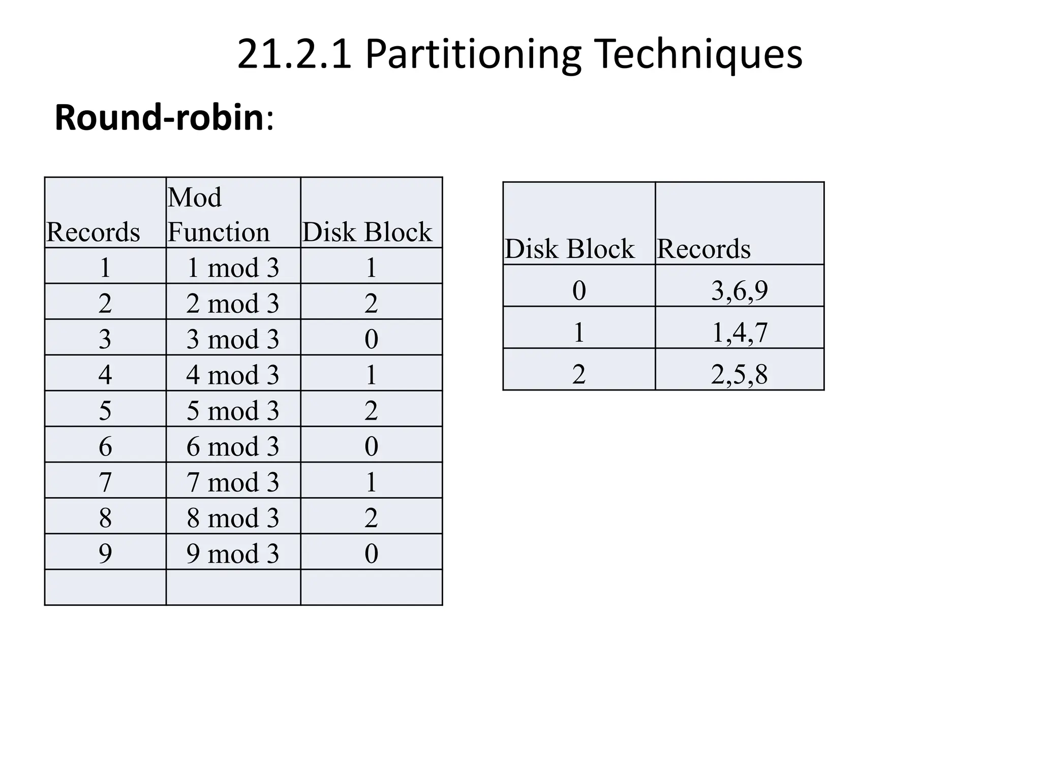
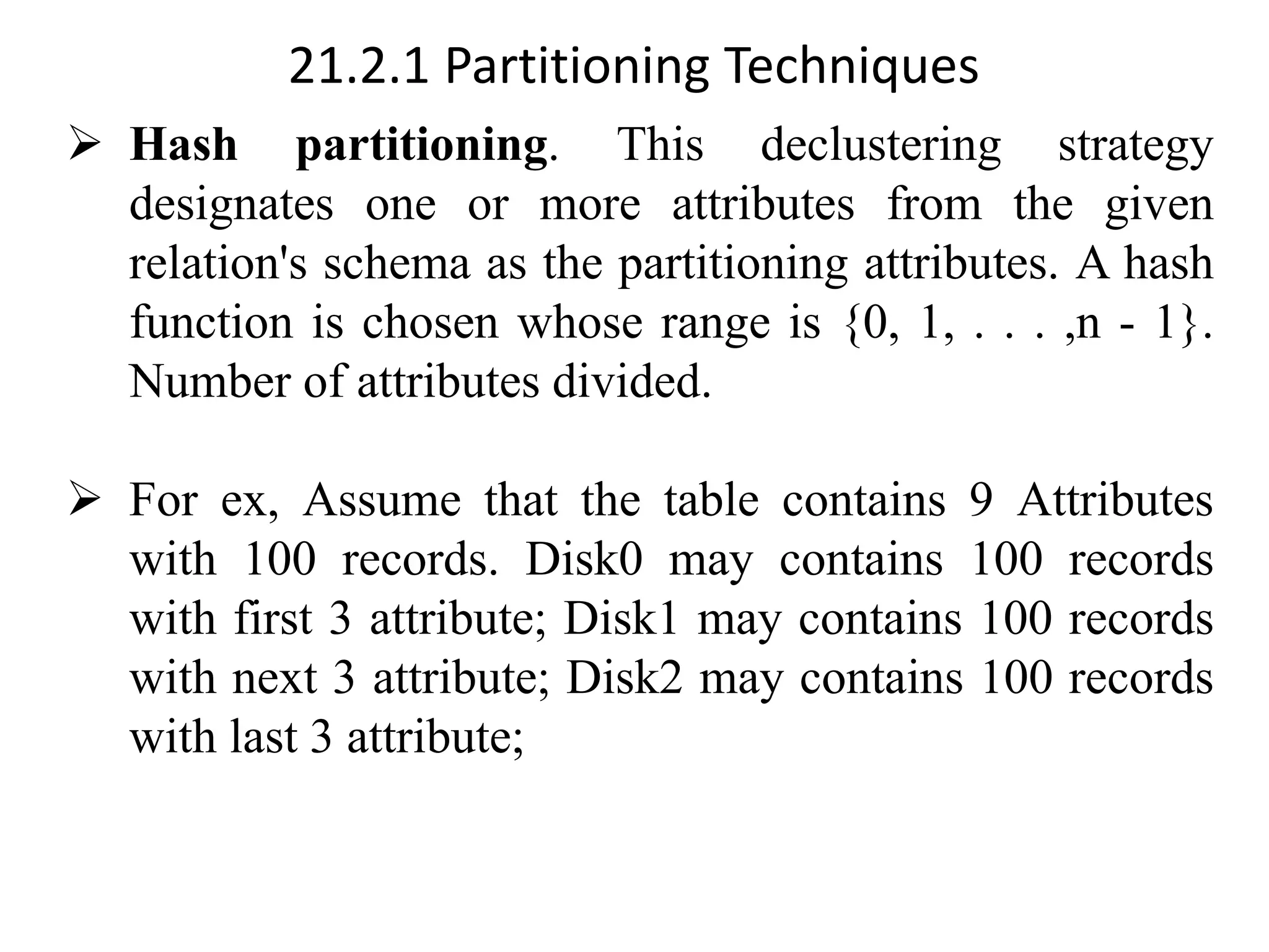
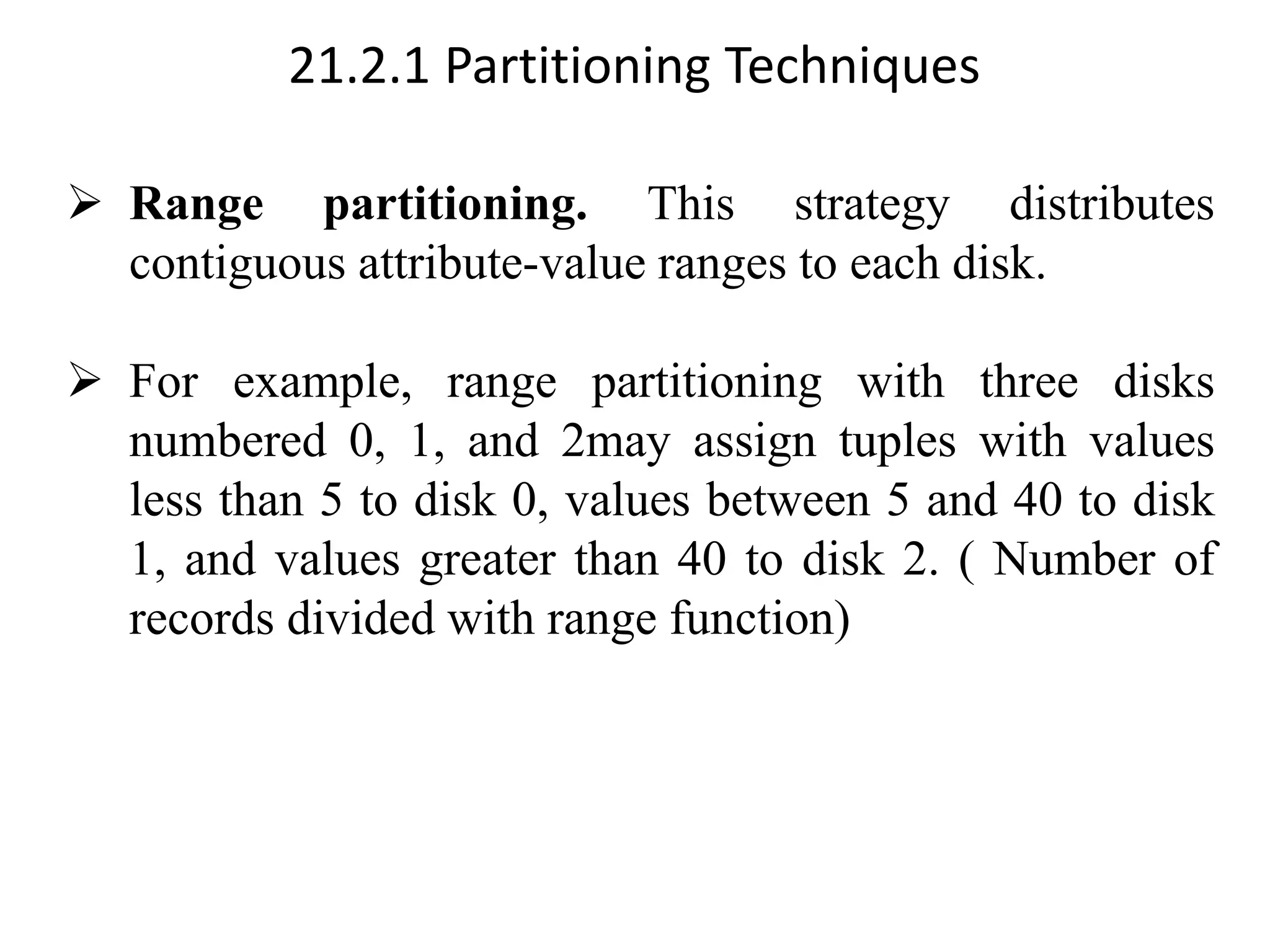
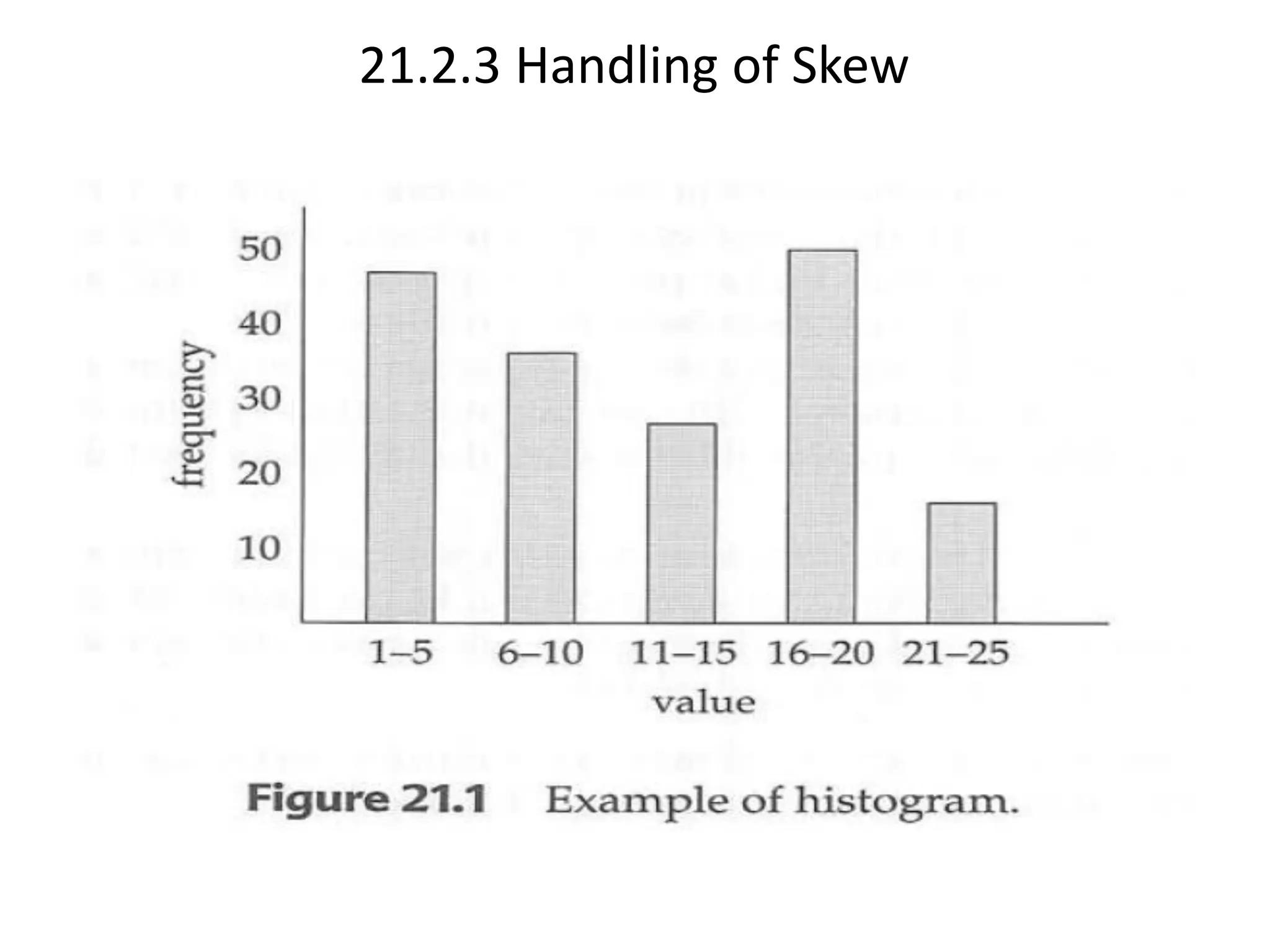
RDBMS - Unit III Chapter 21 Parallel Databases Prepared By Dr. S.Murugan, Associate Professor Department of Computer Science, AlagappaGovernment Arts College, Karaikudi. (Affiliated by AlagappaUniversity) Mailid: muruganjit@gmail.com Reference Book: Database System Concepts by Abraham Silberschatz, Henry F.Korth , S. Sudharshan
21.1 Introduction ➢ A large number of computers used by the organization. ➢ Organizations are using large volumes of data-such as data about what items people buy, what Web links users click on, and when people make telephone calls- to plan their activities and pricing. ➢ As microprocessors have become cheap, parallel machines have become common and relatively inexpensive
21.2 lO Parallelism ➢ I/O parallelism refers to reducing the time required to retrieve relations from disk by partitioning the relations on multiple disks. ➢ The most common form of data partitioning is horizontal partitioning. ➢ In horizontal partitioning, the tuples of a relation are divided (or declustered) among many disks.
21.2.1 Partitioning Techniques ➢ There are three basic data-partitioning strategies are discussed here. Assume that there are n disks, Do, D1,. . . , Dn-1, across which the data are to be partitioned. ➢ Round-robin. This strategy scans the relation in any order and sends the ith tuple to disk number Di mod n. Each disk has approximately the same number of tuples as the others. (Number of records divided with mod function)
21.2.1 Partitioning Techniques Round-robin: Records Mod Function Disk Block 1 1 mod 3 1 2 2 mod 3 2 3 3 mod 3 0 4 4 mod 3 1 5 5 mod 3 2 6 6 mod 3 0 7 7 mod 3 1 8 8 mod 3 2 9 9 mod 3 0 Disk Block Records 0 3,6,9 1 1,4,7 2 2,5,8
21.2.1 Partitioning Techniques ➢ Hash partitioning. This declustering strategy designates one or more attributes from the given relation's schema as the partitioning attributes. A hash function is chosen whose range is {0, 1, . . . ,n - 1}. Number of attributes divided. ➢ For ex, Assume that the table contains 9 Attributes with 100 records. Disk0 may contains 100 records with first 3 attribute; Disk1 may contains 100 records with next 3 attribute; Disk2 may contains 100 records with last 3 attribute;
21.2.1 Partitioning Techniques ➢ Range partitioning. This strategy distributes contiguous attribute-value ranges to each disk. ➢ For example, range partitioning with three disks numbered 0, 1, and 2may assign tuples with values less than 5 to disk 0, values between 5 and 40 to disk 1, and values greater than 40 to disk 2. ( Number of records divided with range function)
21.2.2 Comparison of Partitioning Techniques ➢ Once a relation has been partitioned among several disks, we can retrieve it in parallel, using all the disks. ➢ Similarly, when a relation is being partitioned, it can be written to multiple disks in parallel. ➢ The transfer rates for reading or writing an entire relation are much faster with I/O parallelism. ➢ Reading an entire relation, or scanning a relation, is only one kind of access to data.
21.2.2 Comparison of Partitioning Techniques ➢ Access to data can be classified as follows: 1. Scanning the entire relation 2. Locating a tuple associatively (for example, employee_nam=e " Campbell"); these queries, called point queries, seek tuples that have a specified value for a specific attribute. 3. Locating all tuples for which the value of a given attribute lies within a specified range (for example, 10000 I salary < 20000); these queries are called range queries
21.2.3 Handling of Skew ➢ When a relation is partitioned (by a technique other than round-robin), there may be a skew in the distribution of tuples, with a high percentage of tuples placed in some partitions and fewer tuples in other partitions. ➢ The skew may be classified as: ➢ Attribute-value skew ➢ Partition skew
21.2.3 Handling of Skew ➢ Attribute-value skew refers to the fact that some values appear in the partitioning attributes of many tuples. ➢ Partition skew refers to the fact that there may be load imbalance in the partitioning.
21.2.3 Handling of Skew ➢ A balanced range-partitioning vector can be constructed by sorting: ➢ The relation is first sorted on the partitioning attributes. ➢ The relation is then scanned in sorted order. ➢ After every 1/n of the relation has been read, the value of the partitioning attribute of the next tuple is added to the partition vector. Here, n denotes the number of partitions to be constructed.
21.2.3 Handling of Skew ➢ In case there are many tuples with the same value for the partitioning attribute, the technique can still result in some skew. ➢ The main disadvantage of this method is the extra I/O overhead incurred in doing the initial sort. ➢ The I/O overhead for constructing balanced range- partition vectors can be reduced by constructing and storing a frequency table, or histogram, of the attribute values for each attribute of each relation. ➢ Figure 21.1 shows an example of a histogram for an integer-valued attribute that takes values in the range 1 to 25.
21.2.3 Handling of Skew
21.2.3 Handling of Skew ➢ In case there are many tuples with the same value for the partitioning attribute, the technique can still result in some skew. ➢ The main disadvantage of this method is the extra I/O overhead incurred in doing the initial sort. ➢ The I/O overhead for constructing balanced range- partition vectors can be reduced by constructing and storing a frequency table, or histogram, of the attribute values for each attribute of each relation. ➢ Figure 21.1 shows an example of a histogram for an integer-valued attribute that takes values in the range 1 to 25.
21.3 Interquery Parallelism ➢ In interquery parallelism, different queries or transactions execute in parallel with one another. ➢ Transaction throughput and scaleup can be increased by this form of parallelism. ➢ Interquery parallelism is the easiest form of parallelism to support in a database system- particularly in a shared-memory parallel system. Lock tables and Log information are maintained in the same memory. ➢ Supporting interquery parallelism is more complicated in a shared-disk or shared nothing architecture.
21.3 Interquery Parallelism ➢ Processors have to perform some tasks, such as locking and logging, in a coordinated fashion, and that requires that they pass messages to each other. ➢ A parallel database system must also ensure that two processors do not update the same data independently at the same time. ➢ When a processor accesses or updates data, the database system must ensure that the processor has the latest version of the data in its buffer pool. The problem of ensuring that the version is the latest is known as the cache-coherency problem.
21.4 Intraquery Parallelism It is the form of parallelism where Single Query is executed in parallel on many processors. Advantages ➢ To speed up a single complex long running queries. ➢ Best suited for complex scientific calculations (queries). Supported Parallel Database Architectures SharedMemory, Shared Disk and Shared Nothing parallel architectures are supported. We need not worry about locking and logging as because it involves parallelizing single query.
21.4 Intraquery Parallelism Types Intra-operation parallelism – the process of speeding up a query through parallelizing the execution of individual operations. The operations which can be parallelized are Sort, Join, Projection, Selection and so on. Inter-operation parallelism – the process of speeding up a query through parallelizing various operations which are part of the query. For example, a query which involves join of 4 tables can be executed in parallel in two processors in such a way that each processor shall join two relations locally and the result1 and result2 can be joined further to produce the final result.

Lecture Notes Unit3 chapter21 - parallel databases

  • 1.
    RDBMS - UnitIII Chapter 21 Parallel Databases Prepared By Dr. S.Murugan, Associate Professor Department of Computer Science, AlagappaGovernment Arts College, Karaikudi. (Affiliated by AlagappaUniversity) Mailid: muruganjit@gmail.com Reference Book: Database System Concepts by Abraham Silberschatz, Henry F.Korth , S. Sudharshan
  • 2.
    21.1 Introduction ➢ Alarge number of computers used by the organization. ➢ Organizations are using large volumes of data-such as data about what items people buy, what Web links users click on, and when people make telephone calls- to plan their activities and pricing. ➢ As microprocessors have become cheap, parallel machines have become common and relatively inexpensive
  • 3.
    21.2 lO Parallelism ➢I/O parallelism refers to reducing the time required to retrieve relations from disk by partitioning the relations on multiple disks. ➢ The most common form of data partitioning is horizontal partitioning. ➢ In horizontal partitioning, the tuples of a relation are divided (or declustered) among many disks.
  • 4.
    21.2.1 Partitioning Techniques ➢There are three basic data-partitioning strategies are discussed here. Assume that there are n disks, Do, D1,. . . , Dn-1, across which the data are to be partitioned. ➢ Round-robin. This strategy scans the relation in any order and sends the ith tuple to disk number Di mod n. Each disk has approximately the same number of tuples as the others. (Number of records divided with mod function)
  • 5.
    21.2.1 Partitioning Techniques Round-robin: Records Mod FunctionDisk Block 1 1 mod 3 1 2 2 mod 3 2 3 3 mod 3 0 4 4 mod 3 1 5 5 mod 3 2 6 6 mod 3 0 7 7 mod 3 1 8 8 mod 3 2 9 9 mod 3 0 Disk Block Records 0 3,6,9 1 1,4,7 2 2,5,8
  • 6.
    21.2.1 Partitioning Techniques ➢Hash partitioning. This declustering strategy designates one or more attributes from the given relation's schema as the partitioning attributes. A hash function is chosen whose range is {0, 1, . . . ,n - 1}. Number of attributes divided. ➢ For ex, Assume that the table contains 9 Attributes with 100 records. Disk0 may contains 100 records with first 3 attribute; Disk1 may contains 100 records with next 3 attribute; Disk2 may contains 100 records with last 3 attribute;
  • 7.
    21.2.1 Partitioning Techniques ➢Range partitioning. This strategy distributes contiguous attribute-value ranges to each disk. ➢ For example, range partitioning with three disks numbered 0, 1, and 2may assign tuples with values less than 5 to disk 0, values between 5 and 40 to disk 1, and values greater than 40 to disk 2. ( Number of records divided with range function)
  • 8.
    21.2.2 Comparison ofPartitioning Techniques ➢ Once a relation has been partitioned among several disks, we can retrieve it in parallel, using all the disks. ➢ Similarly, when a relation is being partitioned, it can be written to multiple disks in parallel. ➢ The transfer rates for reading or writing an entire relation are much faster with I/O parallelism. ➢ Reading an entire relation, or scanning a relation, is only one kind of access to data.
  • 9.
    21.2.2 Comparison ofPartitioning Techniques ➢ Access to data can be classified as follows: 1. Scanning the entire relation 2. Locating a tuple associatively (for example, employee_nam=e " Campbell"); these queries, called point queries, seek tuples that have a specified value for a specific attribute. 3. Locating all tuples for which the value of a given attribute lies within a specified range (for example, 10000 I salary < 20000); these queries are called range queries
  • 10.
    21.2.3 Handling ofSkew ➢ When a relation is partitioned (by a technique other than round-robin), there may be a skew in the distribution of tuples, with a high percentage of tuples placed in some partitions and fewer tuples in other partitions. ➢ The skew may be classified as: ➢ Attribute-value skew ➢ Partition skew
  • 11.
    21.2.3 Handling ofSkew ➢ Attribute-value skew refers to the fact that some values appear in the partitioning attributes of many tuples. ➢ Partition skew refers to the fact that there may be load imbalance in the partitioning.
  • 12.
    21.2.3 Handling ofSkew ➢ A balanced range-partitioning vector can be constructed by sorting: ➢ The relation is first sorted on the partitioning attributes. ➢ The relation is then scanned in sorted order. ➢ After every 1/n of the relation has been read, the value of the partitioning attribute of the next tuple is added to the partition vector. Here, n denotes the number of partitions to be constructed.
  • 13.
    21.2.3 Handling ofSkew ➢ In case there are many tuples with the same value for the partitioning attribute, the technique can still result in some skew. ➢ The main disadvantage of this method is the extra I/O overhead incurred in doing the initial sort. ➢ The I/O overhead for constructing balanced range- partition vectors can be reduced by constructing and storing a frequency table, or histogram, of the attribute values for each attribute of each relation. ➢ Figure 21.1 shows an example of a histogram for an integer-valued attribute that takes values in the range 1 to 25.
  • 14.
  • 15.
    21.2.3 Handling ofSkew ➢ In case there are many tuples with the same value for the partitioning attribute, the technique can still result in some skew. ➢ The main disadvantage of this method is the extra I/O overhead incurred in doing the initial sort. ➢ The I/O overhead for constructing balanced range- partition vectors can be reduced by constructing and storing a frequency table, or histogram, of the attribute values for each attribute of each relation. ➢ Figure 21.1 shows an example of a histogram for an integer-valued attribute that takes values in the range 1 to 25.
  • 16.
    21.3 Interquery Parallelism ➢In interquery parallelism, different queries or transactions execute in parallel with one another. ➢ Transaction throughput and scaleup can be increased by this form of parallelism. ➢ Interquery parallelism is the easiest form of parallelism to support in a database system- particularly in a shared-memory parallel system. Lock tables and Log information are maintained in the same memory. ➢ Supporting interquery parallelism is more complicated in a shared-disk or shared nothing architecture.
  • 17.
    21.3 Interquery Parallelism ➢Processors have to perform some tasks, such as locking and logging, in a coordinated fashion, and that requires that they pass messages to each other. ➢ A parallel database system must also ensure that two processors do not update the same data independently at the same time. ➢ When a processor accesses or updates data, the database system must ensure that the processor has the latest version of the data in its buffer pool. The problem of ensuring that the version is the latest is known as the cache-coherency problem.
  • 18.
    21.4 Intraquery Parallelism Itis the form of parallelism where Single Query is executed in parallel on many processors. Advantages ➢ To speed up a single complex long running queries. ➢ Best suited for complex scientific calculations (queries). Supported Parallel Database Architectures SharedMemory, Shared Disk and Shared Nothing parallel architectures are supported. We need not worry about locking and logging as because it involves parallelizing single query.
  • 19.
    21.4 Intraquery Parallelism Types Intra-operationparallelism – the process of speeding up a query through parallelizing the execution of individual operations. The operations which can be parallelized are Sort, Join, Projection, Selection and so on. Inter-operation parallelism – the process of speeding up a query through parallelizing various operations which are part of the query. For example, a query which involves join of 4 tables can be executed in parallel in two processors in such a way that each processor shall join two relations locally and the result1 and result2 can be joined further to produce the final result.