parallel database architecture Slide by Rizvee

Parallel Databases, Processing and Query Optimizations 1 Redwan Ahmed Rizvee (Chapter 18, 6th Edition, Database Systems & Concepts) https://rizveeredwan.github.io/

Definition & Purpose ● Core Concept: Interquery parallelism executes multiple, distinct queries or transactions simultaneously within a database system, leveraging multiple processing units. This concurrent execution maximizes hardware resource utilization. ● Primary Goal: Significantly increase transaction throughput (transactions per second, TPS). By running transactions in parallel, the system handles a high volume of user requests, crucial for applications like e-commerce during peak loads. ● Important Caveat: It does not improve individual transaction response times. A single query's execution time remains largely unchanged; the benefit is increased overall capacity, not reduced latency for single tasks. This distinguishes it from intraquery parallelism. ● Main Application: Primarily used to scale up transaction-processing systems for a larger number of transactions per second. It's ideal for high-volume, short-lived transactions in Online Transaction Processing (OLTP) systems (e.g., banking, airline reservations), preventing bottlenecks under heavy load. 3

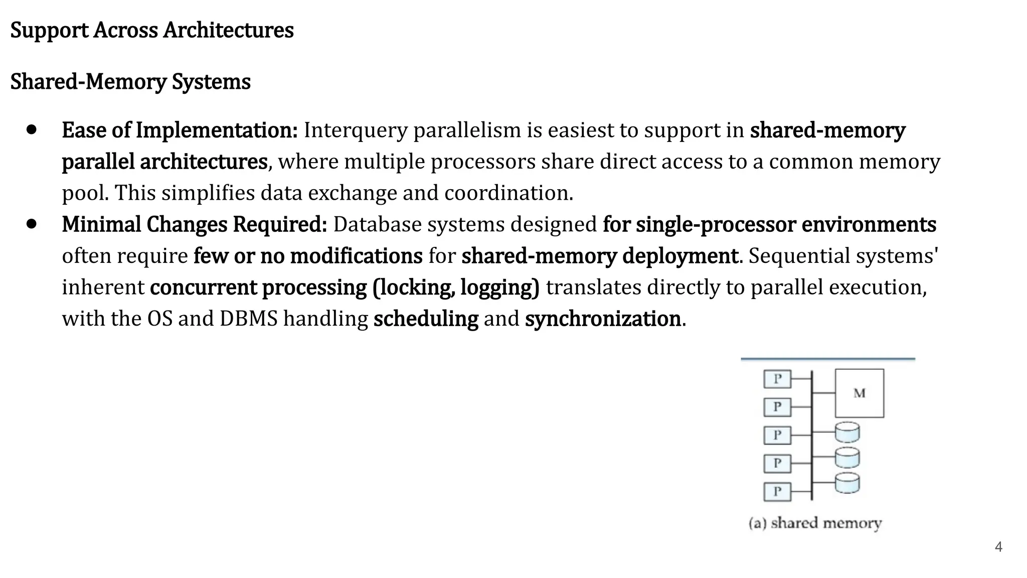
Support Across Architectures Shared-Memory Systems ● Ease of Implementation: Interquery parallelism is easiest to support in shared-memory parallel architectures, where multiple processors share direct access to a common memory pool. This simplifies data exchange and coordination. ● Minimal Changes Required: Database systems designed for single-processor environments often require few or no modifications for shared-memory deployment. Sequential systems' inherent concurrent processing (locking, logging) translates directly to parallel execution, with the OS and DBMS handling scheduling and synchronization. 4

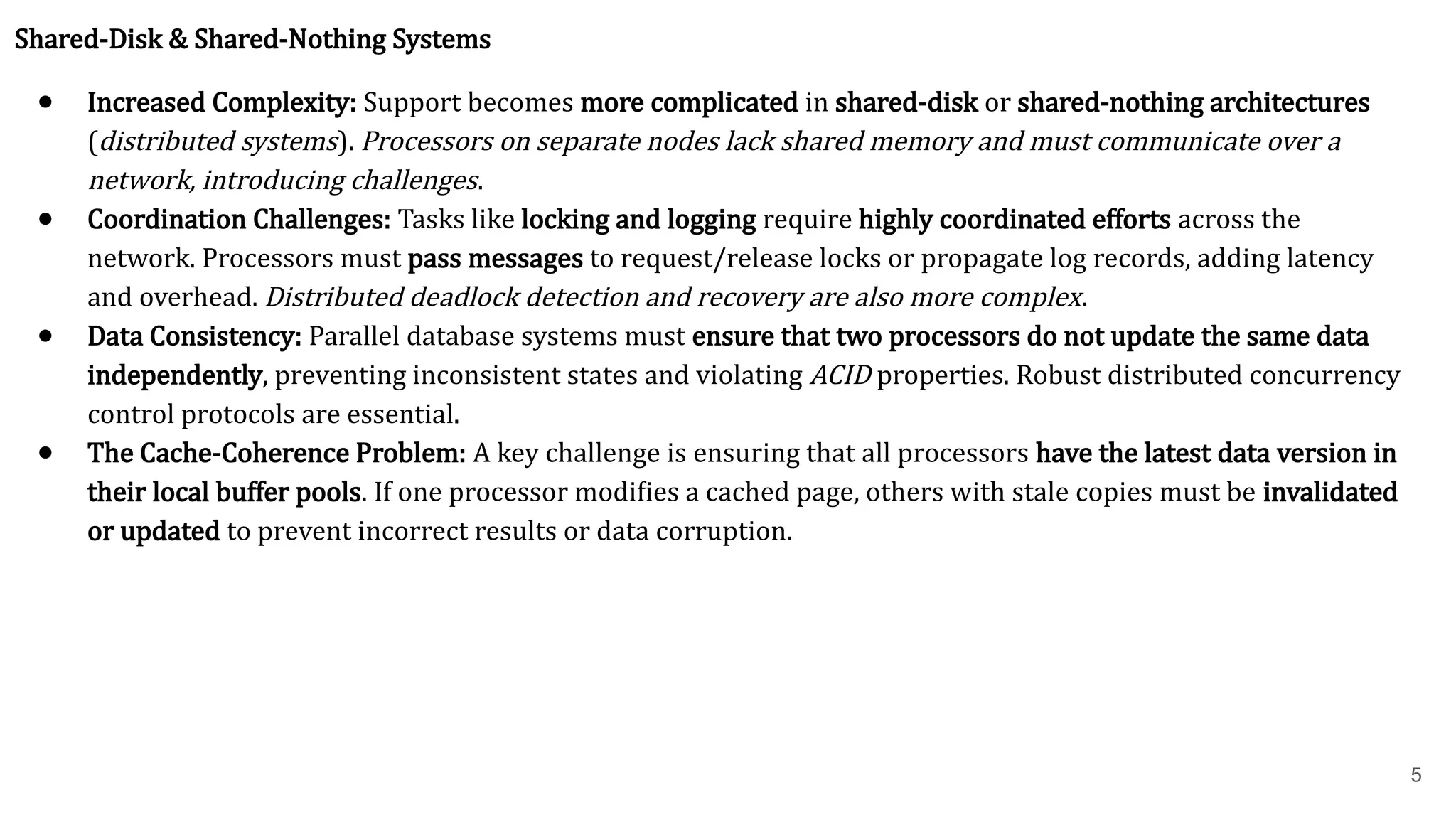
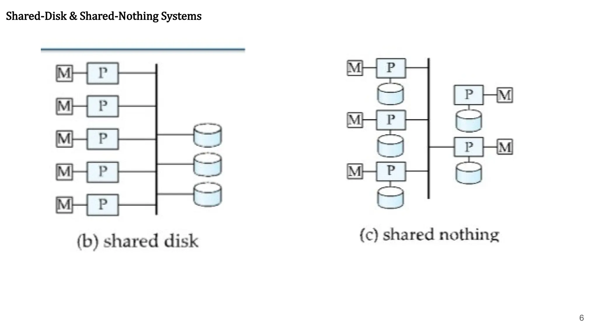
5 Shared-Disk & Shared-Nothing Systems ● Increased Complexity: Support becomes more complicated in shared-disk or shared-nothing architectures (distributed systems). Processors on separate nodes lack shared memory and must communicate over a network, introducing challenges. ● Coordination Challenges: Tasks like locking and logging require highly coordinated efforts across the network. Processors must pass messages to request/release locks or propagate log records, adding latency and overhead. Distributed deadlock detection and recovery are also more complex. ● Data Consistency: Parallel database systems must ensure that two processors do not update the same data independently, preventing inconsistent states and violating ACID properties. Robust distributed concurrency control protocols are essential. ● The Cache-Coherence Problem: A key challenge is ensuring that all processors have the latest data version in their local buffer pools. If one processor modifies a cached page, others with stale copies must be invalidated or updated to prevent incorrect results or data corruption.

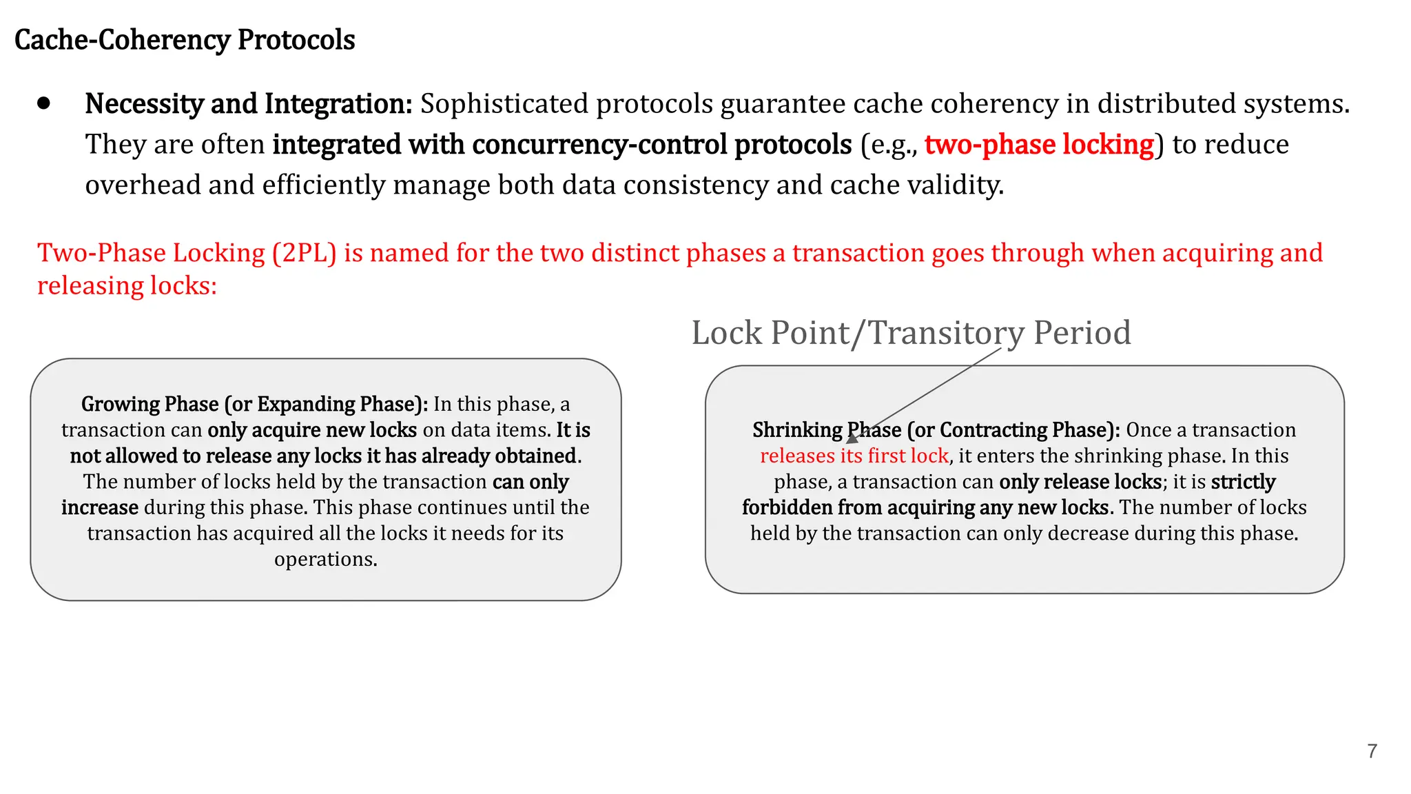
6 Shared-Disk & Shared-Nothing Systems

7 Cache-Coherency Protocols ● Necessity and Integration: Sophisticated protocols guarantee cache coherency in distributed systems. They are often integrated with concurrency-control protocols (e.g., two-phase locking) to reduce overhead and efficiently manage both data consistency and cache validity. Two-Phase Locking (2PL) is named for the two distinct phases a transaction goes through when acquiring and releasing locks: Growing Phase (or Expanding Phase): In this phase, a transaction can only acquire new locks on data items. It is not allowed to release any locks it has already obtained. The number of locks held by the transaction can only increase during this phase. This phase continues until the transaction has acquired all the locks it needs for its operations. Shrinking Phase (or Contracting Phase): Once a transaction releases its first lock, it enters the shrinking phase. In this phase, a transaction can only release locks; it is strictly forbidden from acquiring any new locks. The number of locks held by the transaction can only decrease during this phase. Lock Point/Transitory Period

8 A simple protocol for shared-disk systems: 1. Before Any Read or Write: A transaction locks the page (shared/exclusive) and immediately reads the most recent copy from the shared disk. This "read-on-lock" ensures the latest committed version. 2. Before Exclusive Lock Release: The transaction flushes the modified page to the shared disk for persistence, then releases the lock. Limitations of Simple Protocols: This "disk-centric" approach incurs considerable overhead due to repeated disk I/O, leading to I/O contention and performance degradation, especially for "hot" pages. More Complex Protocols: To mitigate I/O, these protocols do not necessarily write pages to disk when exclusive locks are released. Instead, they often use an invalidation-based approach, sending messages to invalidate other processors' cached copies. When a lock is obtained, the most recent page version is fetched directly from another processor's buffer pool via efficient inter-processor communication ("cache-to-cache transfer"), minimizing disk access.

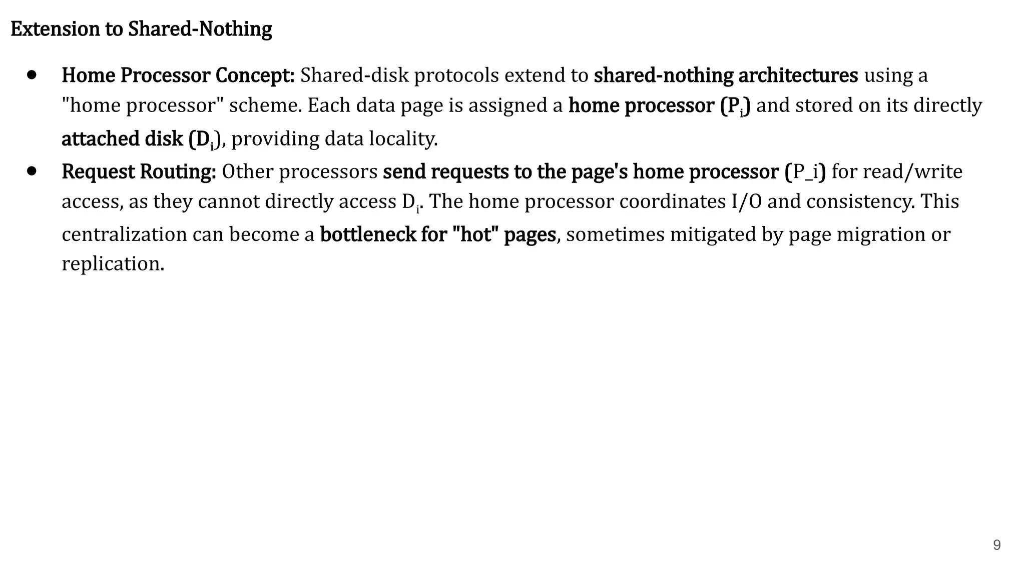
9 Extension to Shared-Nothing ● Home Processor Concept: Shared-disk protocols extend to shared-nothing architectures using a "home processor" scheme. Each data page is assigned a home processor (Pi) and stored on its directly attached disk (Di), providing data locality. ● Request Routing: Other processors send requests to the page's home processor (P_i) for read/write access, as they cannot directly access Di. The home processor coordinates I/O and consistency. This centralization can become a bottleneck for "hot" pages, sometimes mitigated by page migration or replication.

10 Examples ● Prominent shared-disk parallel database systems supporting interquery parallelism include Oracle and Oracle Rdb. Their robust architectures manage concurrent transactions across multiple nodes, demonstrating the effectiveness of interquery parallelism for high-throughput enterprise applications.

12 Definition & Purpose ● Definition: Execution of a single query in parallel using multiple processors and disks. ● Purpose: Crucial for speeding up long-running queries. ● Contrast: Unlike interquery parallelism (throughput-focused), intraquery parallelism directly reduces single query response times.

13 Sources of Parallelism within a Query 1. Parallelizing Individual Operations (Intraoperation Parallelism) ● Speeding up atomic operations within a query (e.g., sort, select, project, join). ● Example (Sort): For a range-partitioned relation, each partition can be sorted in parallel, then concatenated. 2. Parallelizing Operator Tree Evaluation (Interoperation Parallelism) ● Executing different, independent operations within a query's operator tree in parallel. ● Pipelining: Operations can execute in parallel, with one consuming the output of another as it's generated. Two Forms of Query Parallelization ● Intraoperation Parallelism: Speeds up processing by parallelizing each individual operation. ● Interoperation Parallelism: Speeds up processing by executing different operations in a query expression in parallel Intraoperation parallelism scales better due to the large number of tuples processed per operation relative to few operations in a query.

14 Assumptions for Algorithm Description ● Queries: Assumed to be read-only. ● Architecture Model: Algorithms use a shared-nothing architecture model for clarity, detailing data transfers. ● Simulatable: This model is easily simulatable on shared-memory (via shared memory) and shared-disk (via shared disks) architectures. ● System Setup: Assumes processors (P0 ,P1...,Pn−1 ) and n disks (D0 ,D1...,Dn−1 ), with Diassociated with Pi (extensible to multiple disks per processor).

16 Intraoperation parallelism is natural in database systems due to relations containing large sets of tuples, allowing operations to be executed in parallel on different subsets, offering potentially enormous degrees of parallelism. Parallel Sort ● Suppose we wish to sort a relation residing on N disks (D0 ,D1 ,...,Dn−1 ). ● Case 1: Range-Partitioned Relation: If the relation is already range-partitioned on the sort attributes, each partition can be sorted separately in parallel. The sorted partitions can then be concatenated to form the final sorted relation. Parallel disk access reduces the total read time. ● Case 2: Other Partitioning Methods: If the relation is partitioned in any other way, sorting can be achieved by: 1. Range-partitioning it on the sort attributes first, then sorting each partition separately. 2. Using a parallel version of the external sort-merge algorithm.

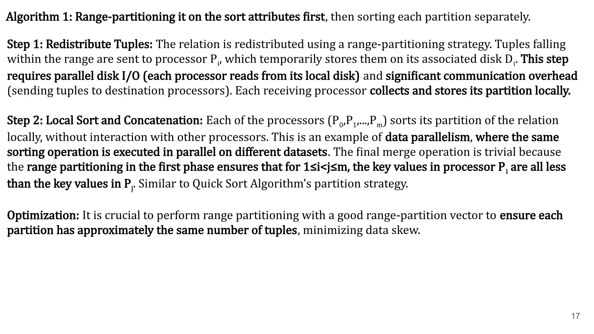
17 Algorithm 1: Range-partitioning it on the sort attributes first, then sorting each partition separately. Step 1: Redistribute Tuples: The relation is redistributed using a range-partitioning strategy. Tuples falling within the range are sent to processor Pi , which temporarily stores them on its associated disk Di . This step requires parallel disk I/O (each processor reads from its local disk) and significant communication overhead (sending tuples to destination processors). Each receiving processor collects and stores its partition locally. Step 2: Local Sort and Concatenation: Each of the processors (P0 ,P1 ,...,Pm ) sorts its partition of the relation locally, without interaction with other processors. This is an example of data parallelism, where the same sorting operation is executed in parallel on different datasets. The final merge operation is trivial because the range partitioning in the first phase ensures that for 1≤i<j≤m, the key values in processor Piare all less than the key values in Pj . Similar to Quick Sort Algorithm’s partition strategy. Optimization: It is crucial to perform range partitioning with a good range-partition vector to ensure each partition has approximately the same number of tuples, minimizing data skew.

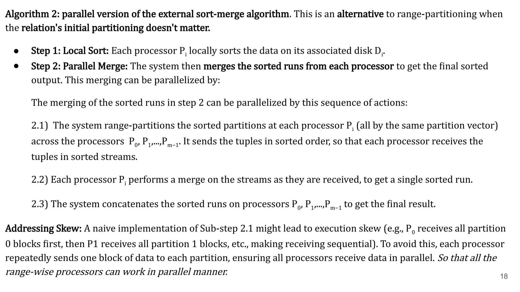
18 Algorithm 2: parallel version of the external sort-merge algorithm. This is an alternative to range-partitioning when the relation's initial partitioning doesn't matter. ● Step 1: Local Sort: Each processor Pi locally sorts the data on its associated disk Di . ● Step 2: Parallel Merge: The system then merges the sorted runs from each processor to get the final sorted output. This merging can be parallelized by: The merging of the sorted runs in step 2 can be parallelized by this sequence of actions: 2.1) The system range-partitions the sorted partitions at each processor Pi (all by the same partition vector) across the processors P0, P1,...,Pm−1. It sends the tuples in sorted order, so that each processor receives the tuples in sorted streams. 2.2) Each processor Pi performs a merge on the streams as they are received, to get a single sorted run. 2.3) The system concatenates the sorted runs on processors P0, P1,...,Pm−1 to get the ﬁnal result. Addressing Skew: A naive implementation of Sub-step 2.1 might lead to execution skew (e.g., P0receives all partition 0 blocks first, then P1receives all partition 1 blocks, etc., making receiving sequential). To avoid this, each processor repeatedly sends one block of data to each partition, ensuring all processors receive data in parallel. So that all the range-wise processors can work in parallel manner.

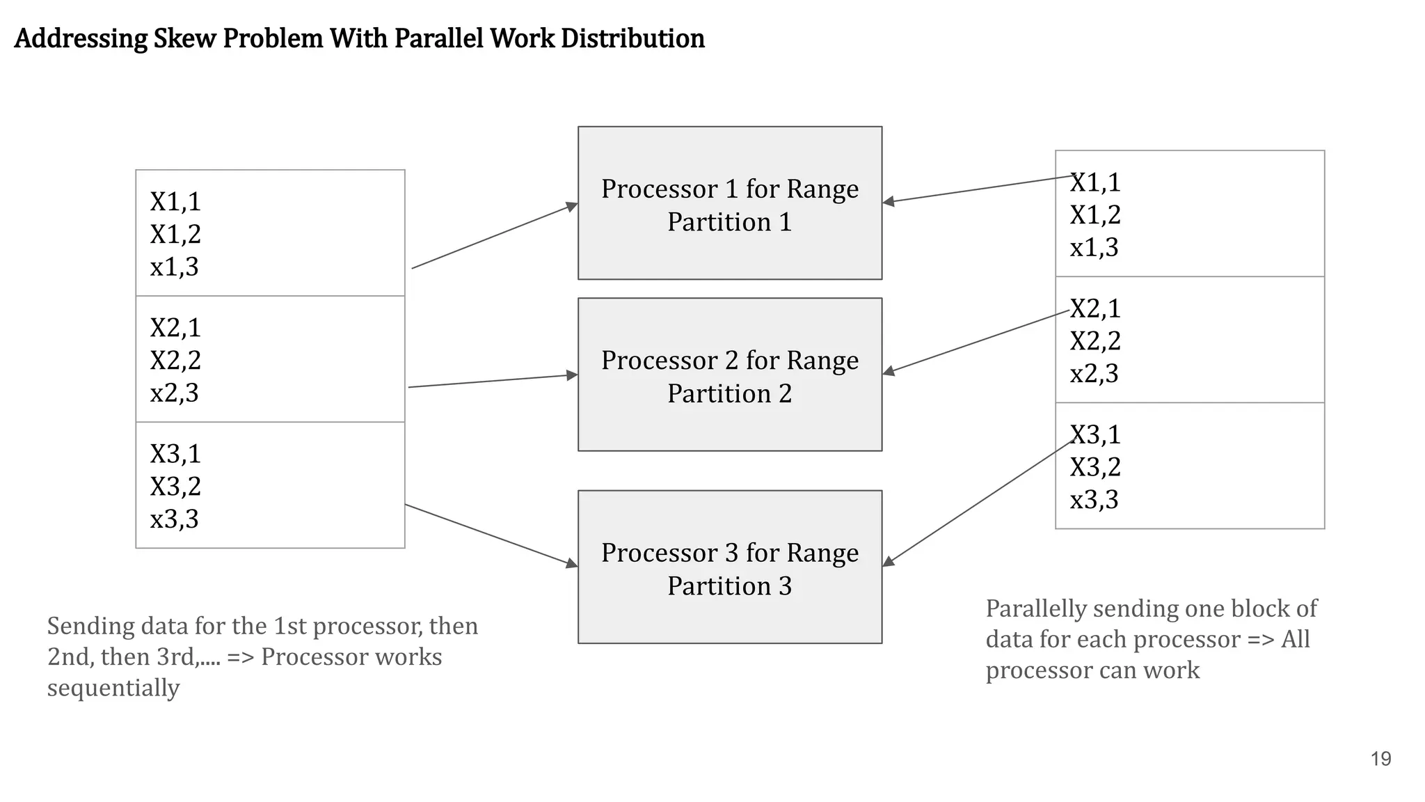
19 X1,1 X1,2 x1,3 X2,1 X2,2 x2,3 X3,1 X3,2 x3,3 Processor 1 for Range Partition 1 Processor 2 for Range Partition 2 Processor 3 for Range Partition 3 X1,1 X1,2 x1,3 X2,1 X2,2 x2,3 X3,1 X3,2 x3,3 Addressing Skew Problem With Parallel Work Distribution Sending data for the 1st processor, then 2nd, then 3rd,.... => Processor works sequentially Parallelly sending one block of data for each processor => All processor can work

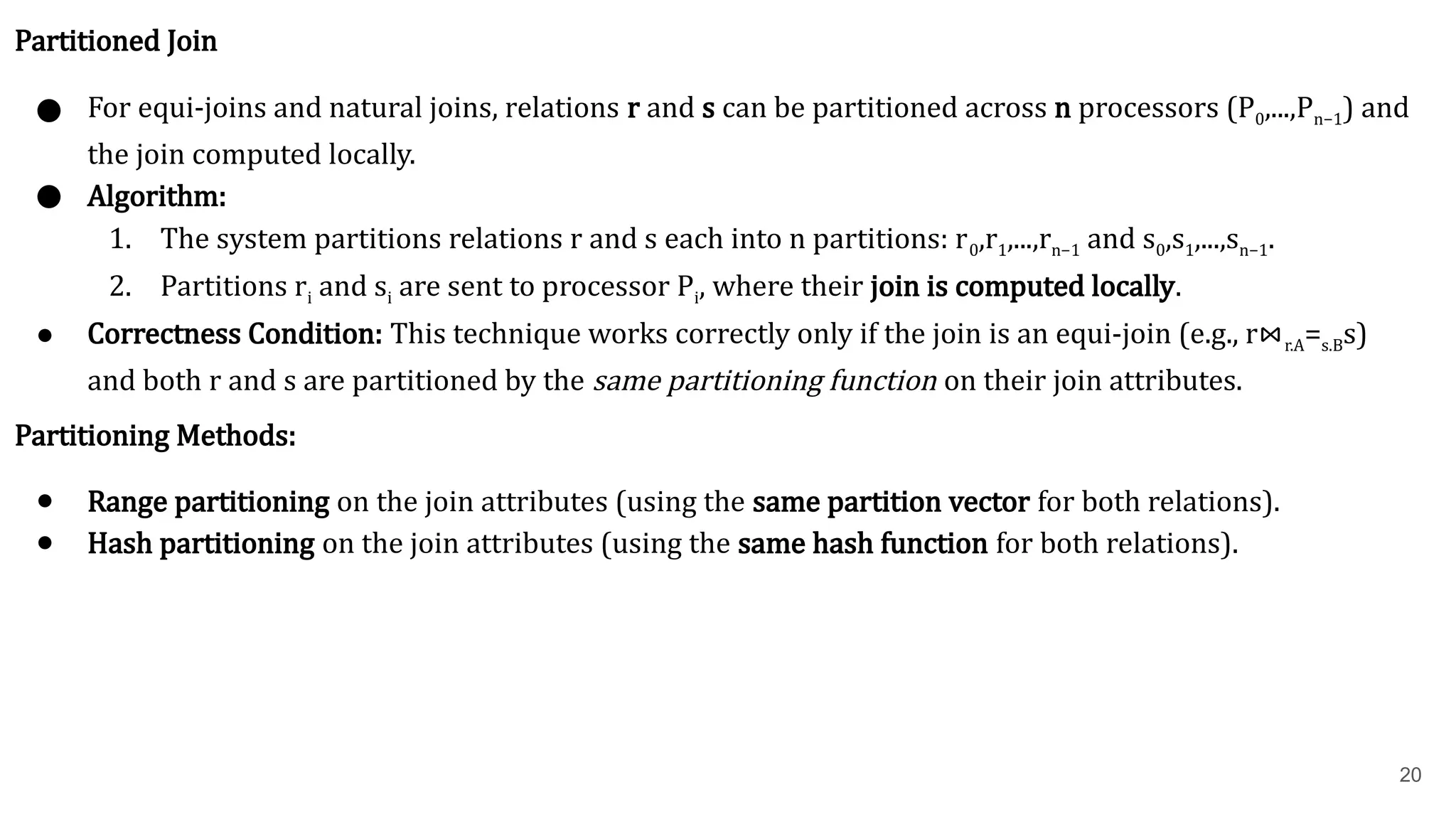
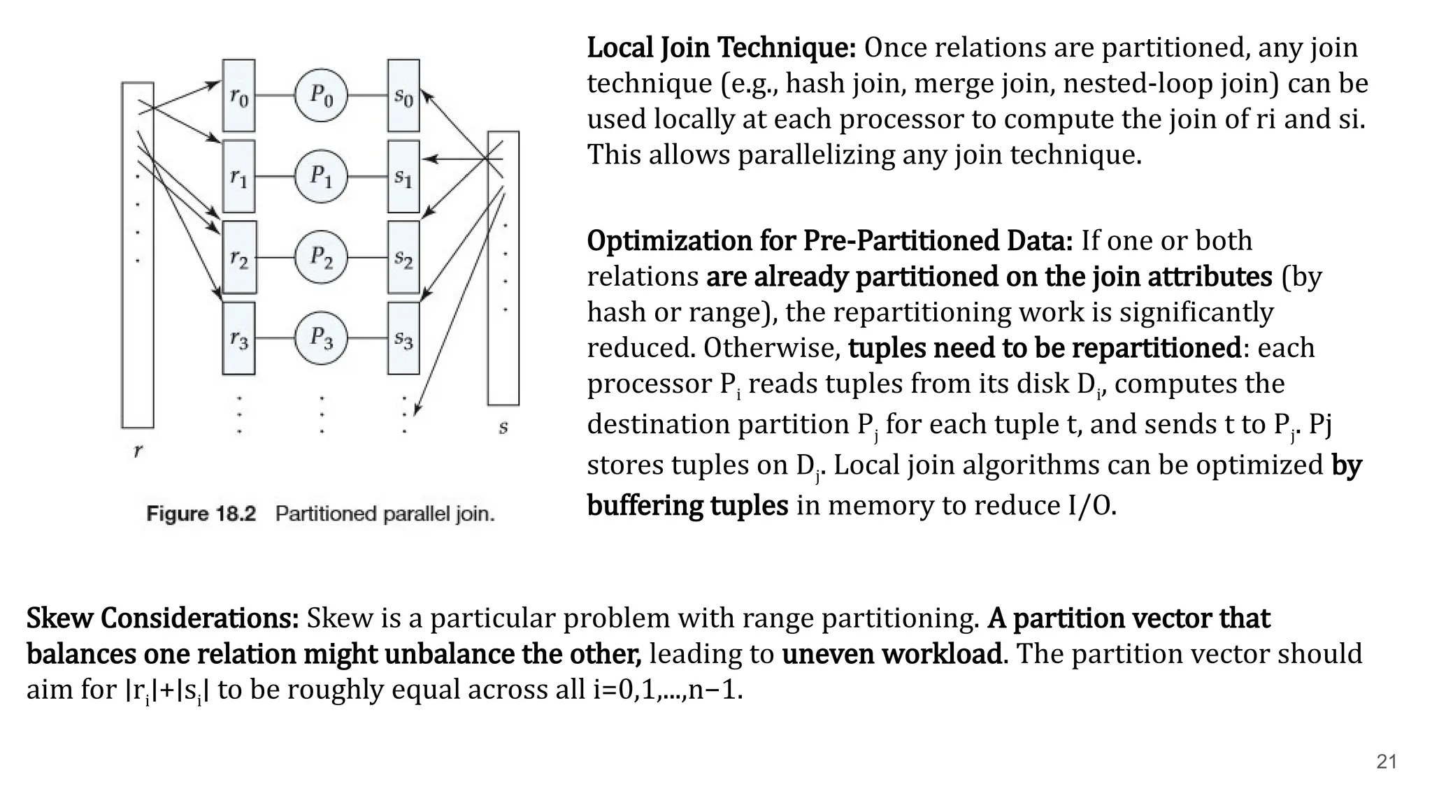
20 Partitioned Join ● For equi-joins and natural joins, relations r and s can be partitioned across n processors (P0 ,...,Pn−1 ) and the join computed locally. ● Algorithm: 1. The system partitions relations r and s each into n partitions: r0 ,r1 ,...,rn−1and s0 ,s1 ,...,sn−1 . 2. Partitions riand siare sent to processor Pi , where their join is computed locally. ● Correctness Condition: This technique works correctly only if the join is an equi-join (e.g., r⋈r.A=s.B s) and both r and s are partitioned by the same partitioning function on their join attributes. Partitioning Methods: ● Range partitioning on the join attributes (using the same partition vector for both relations). ● Hash partitioning on the join attributes (using the same hash function for both relations).

21 Local Join Technique: Once relations are partitioned, any join technique (e.g., hash join, merge join, nested-loop join) can be used locally at each processor to compute the join of riand si . This allows parallelizing any join technique. Optimization for Pre-Partitioned Data: If one or both relations are already partitioned on the join attributes (by hash or range), the repartitioning work is significantly reduced. Otherwise, tuples need to be repartitioned: each processor Pireads tuples from its disk Di , computes the destination partition Pjfor each tuple t, and sends t to Pj . Pj stores tuples on Dj . Local join algorithms can be optimized by buffering tuples in memory to reduce I/O. Skew Considerations: Skew is a particular problem with range partitioning. A partition vector that balances one relation might unbalance the other, leading to uneven workload. The partition vector should aim for ∣ri ∣+∣si ∣ to be roughly equal across all i=0,1,...,n−1.

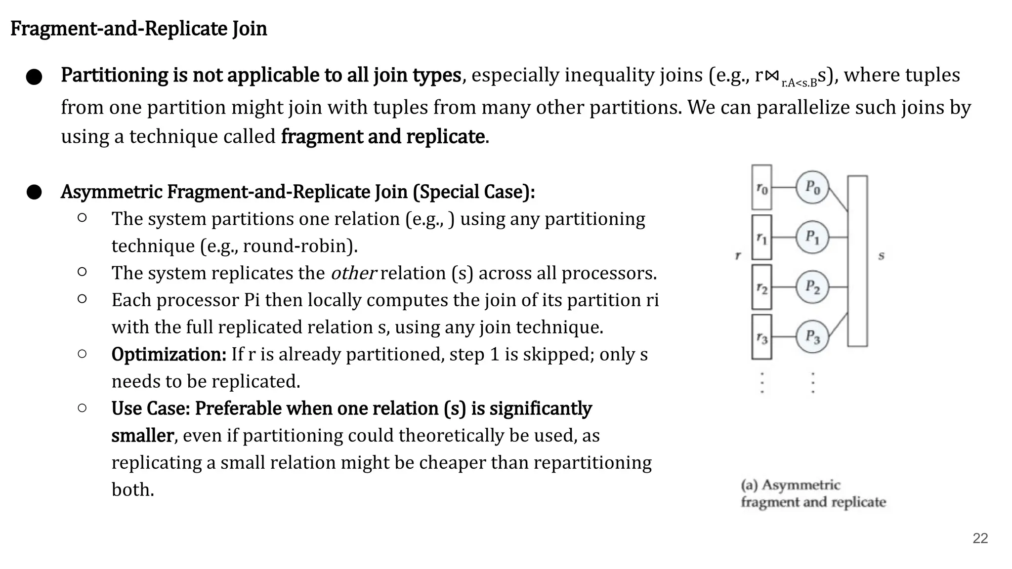
22 Fragment-and-Replicate Join ● Partitioning is not applicable to all join types, especially inequality joins (e.g., r⋈r.A<s.B s), where tuples from one partition might join with tuples from many other partitions. We can parallelize such joins by using a technique called fragment and replicate. ● Asymmetric Fragment-and-Replicate Join (Special Case): ○ The system partitions one relation (e.g., ) using any partitioning technique (e.g., round-robin). ○ The system replicates the other relation (s) across all processors. ○ Each processor Pithen locally computes the join of its partition ri with the full replicated relation s, using any join technique. ○ Optimization: If r is already partitioned, step 1 is skipped; only s needs to be replicated. ○ Use Case: Preferable when one relation (s) is significantly smaller, even if partitioning could theoretically be used, as replicating a small relation might be cheaper than repartitioning both.

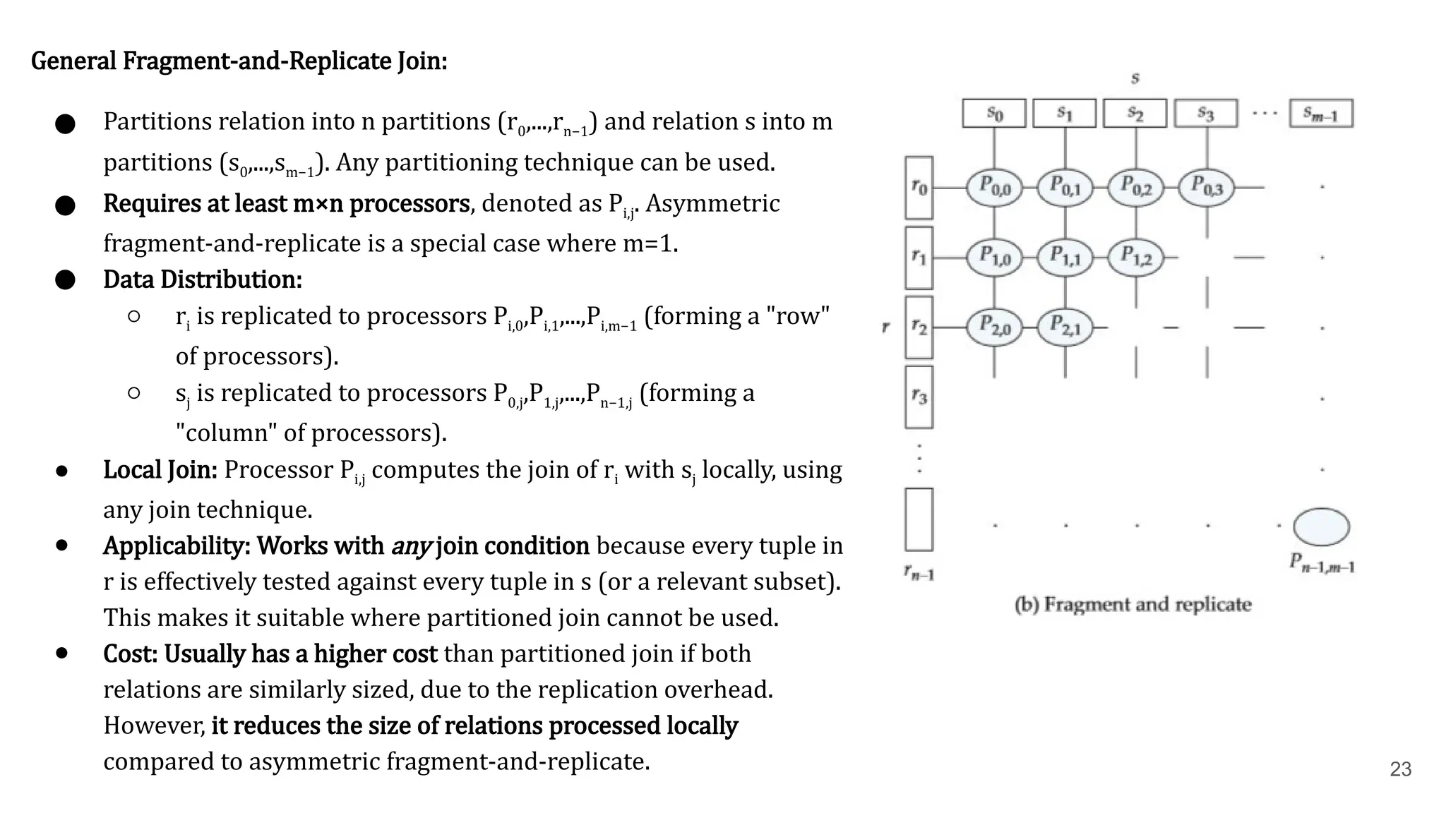
23 General Fragment-and-Replicate Join: ● Partitions relation into n partitions (r0 ,...,rn−1 ) and relation s into m partitions (s0 ,...,sm−1 ). Any partitioning technique can be used. ● Requires at least m×n processors, denoted as Pi,j . Asymmetric fragment-and-replicate is a special case where m=1. ● Data Distribution: ○ riis replicated to processors Pi,0 ,Pi,1 ,...,Pi,m−1 (forming a "row" of processors). ○ sjis replicated to processors P0,j ,P1,j ,...,Pn−1,j(forming a "column" of processors). ● Local Join: Processor Pi,jcomputes the join of riwith sjlocally, using any join technique. ● Applicability: Works with any join condition because every tuple in r is effectively tested against every tuple in s (or a relevant subset). This makes it suitable where partitioned join cannot be used. ● Cost: Usually has a higher cost than partitioned join if both relations are similarly sized, due to the replication overhead. However, it reduces the size of relations processed locally compared to asymmetric fragment-and-replicate.

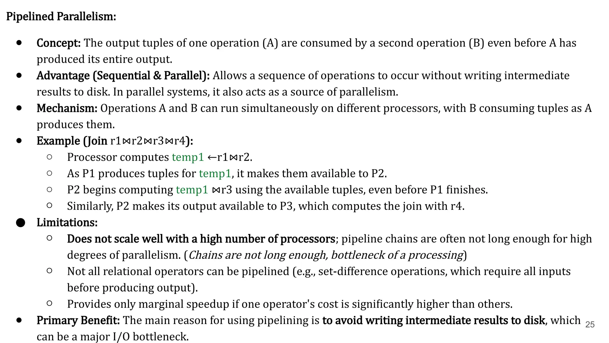
25 Pipelined Parallelism: ● Concept: The output tuples of one operation (A) are consumed by a second operation (B) even before A has produced its entire output. ● Advantage (Sequential & Parallel): Allows a sequence of operations to occur without writing intermediate results to disk. In parallel systems, it also acts as a source of parallelism. ● Mechanism: Operations A and B can run simultaneously on different processors, with B consuming tuples as A produces them. ● Example (Join r1 ⋈r2 ⋈r3 ⋈r4 ): ○ Processor computes temp1 ←r1 ⋈r2 . ○ As P1produces tuples for temp1, it makes them available to P2 . ○ P2begins computing temp1 ⋈r3using the available tuples, even before P1finishes. ○ Similarly, P2makes its output available to P3 , which computes the join with r4 . ● Limitations: ○ Does not scale well with a high number of processors; pipeline chains are often not long enough for high degrees of parallelism. (Chains are not long enough, bottleneck of a processing) ○ Not all relational operators can be pipelined (e.g., set-difference operations, which require all inputs before producing output). ○ Provides only marginal speedup if one operator's cost is significantly higher than others. ● Primary Benefit: The main reason for using pipelining is to avoid writing intermediate results to disk, which can be a major I/O bottleneck.

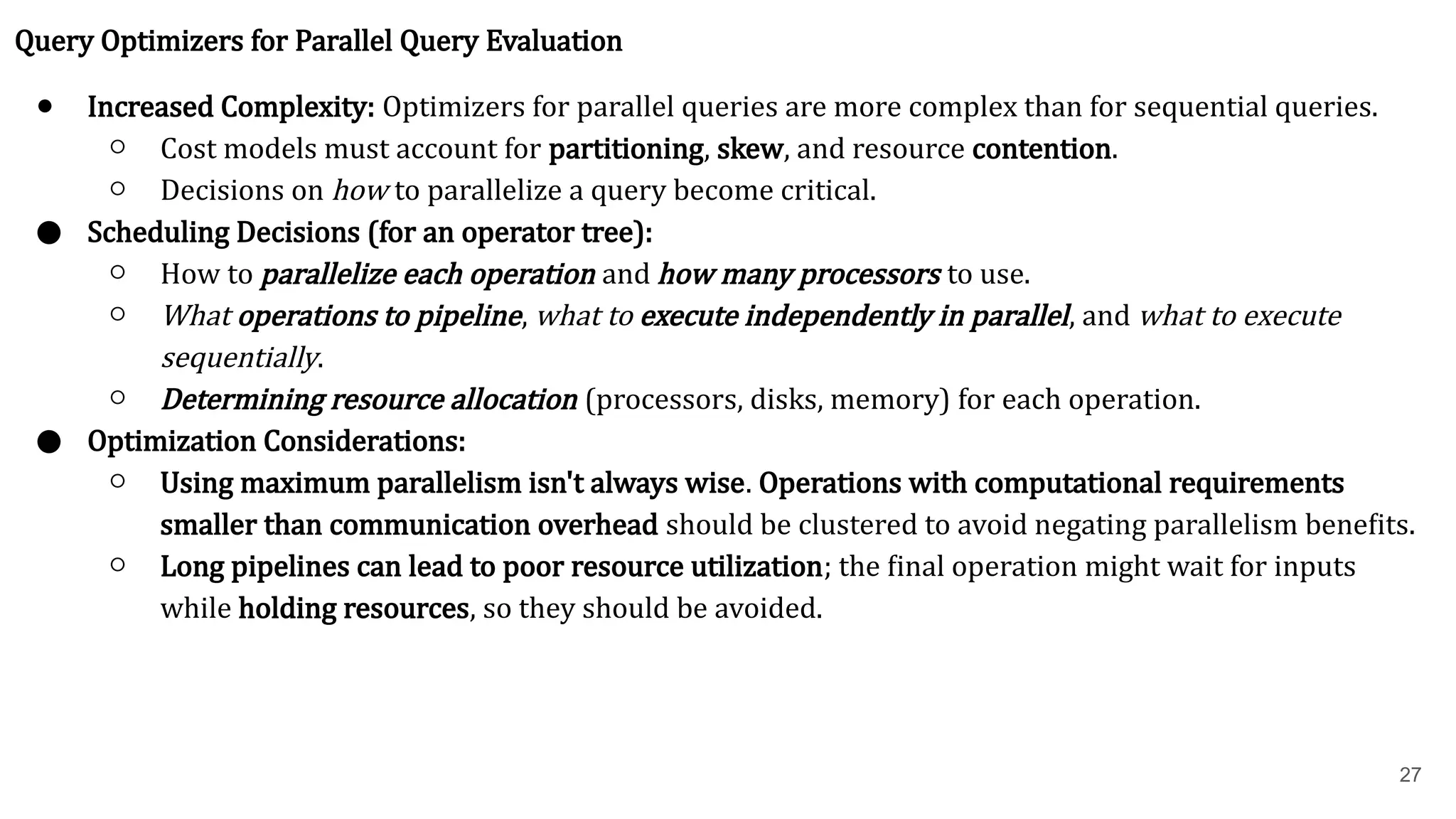
27 Query Optimizers for Parallel Query Evaluation ● Increased Complexity: Optimizers for parallel queries are more complex than for sequential queries. ○ Cost models must account for partitioning, skew, and resource contention. ○ Decisions on how to parallelize a query become critical. ● Scheduling Decisions (for an operator tree): ○ How to parallelize each operation and how many processors to use. ○ What operations to pipeline, what to execute independently in parallel, and what to execute sequentially. ○ Determining resource allocation (processors, disks, memory) for each operation. ● Optimization Considerations: ○ Using maximum parallelism isn't always wise. Operations with computational requirements smaller than communication overhead should be clustered to avoid negating parallelism benefits. ○ Long pipelines can lead to poor resource utilization; the final operation might wait for inputs while holding resources, so they should be avoided.

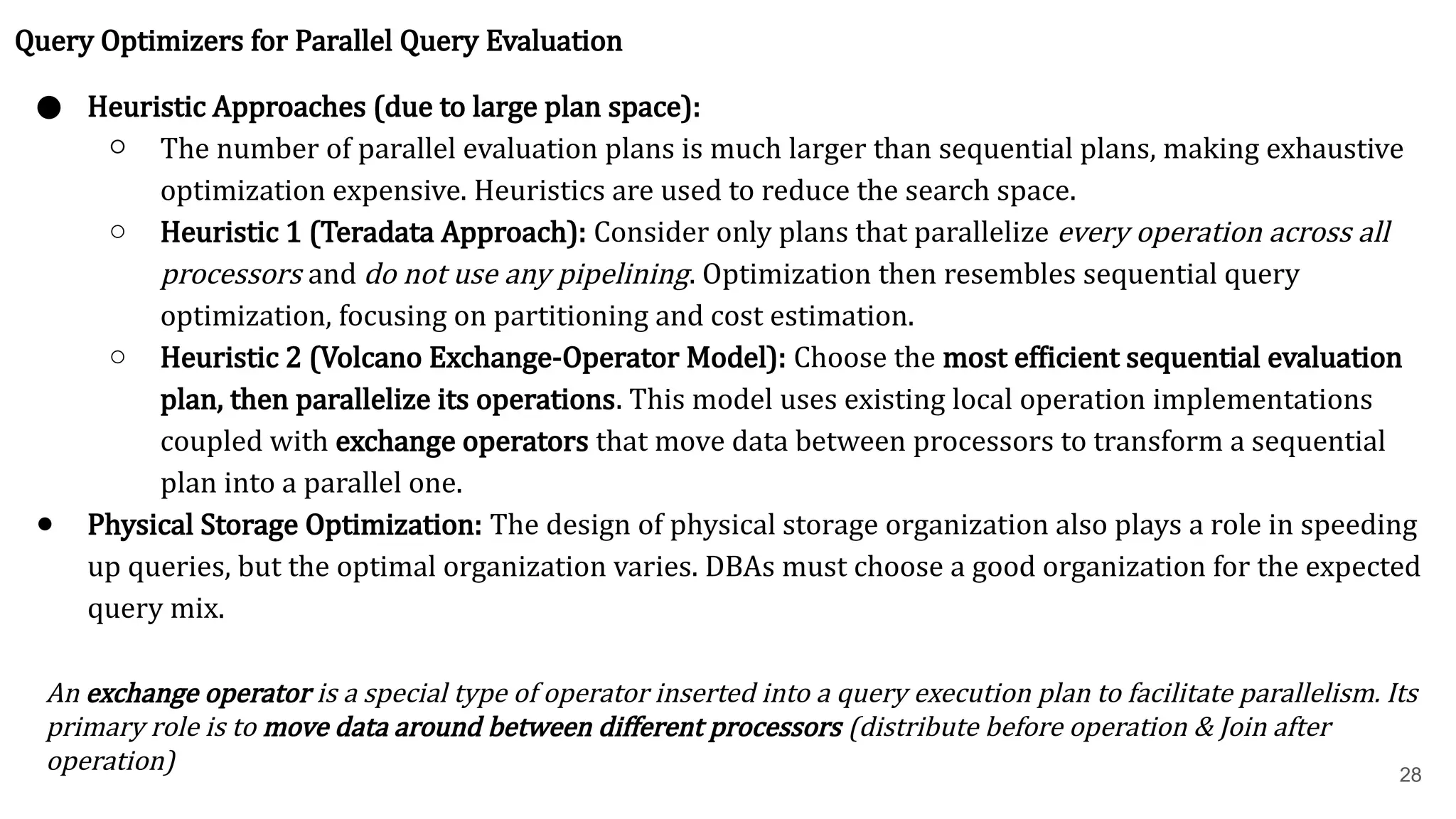
28 Query Optimizers for Parallel Query Evaluation ● Heuristic Approaches (due to large plan space): ○ The number of parallel evaluation plans is much larger than sequential plans, making exhaustive optimization expensive. Heuristics are used to reduce the search space. ○ Heuristic 1 (Teradata Approach): Consider only plans that parallelize every operation across all processors and do not use any pipelining. Optimization then resembles sequential query optimization, focusing on partitioning and cost estimation. ○ Heuristic 2 (Volcano Exchange-Operator Model): Choose the most efficient sequential evaluation plan, then parallelize its operations. This model uses existing local operation implementations coupled with exchange operators that move data between processors to transform a sequential plan into a parallel one. ● Physical Storage Optimization: The design of physical storage organization also plays a role in speeding up queries, but the optimal organization varies. DBAs must choose a good organization for the expected query mix. An exchange operator is a special type of operator inserted into a query execution plan to facilitate parallelism. Its primary role is to move data around between different processors (distribute before operation & Join after operation)

parallel database architecture Slide by Rizvee

More Related Content

Similar to parallel database architecture Slide by Rizvee

Recently uploaded

parallel database architecture Slide by Rizvee