Introduction to matlab lecture 4 of 4

>> pathname = 'C:UsersAyaDesktoppic'; >> for i = 1:10 imagename = strcat(pathname,int2str(i),'.jpg'); I = imread(imagename); M(i) = mean(mean(mean(I)));% RGB image end >> save 'C:UsersAyaDesktopMEANS.mat' M; >> MR=load ('C:UsersAyaDesktopMEANS.mat') MR = M: [93.6082 93.6082 93.6082 93.6082 93.6082] 2

 Matlab plotting › 2D plots › 3D plots  M-Files › Scripts › User defined functions 3

 Matlab has a lot of function for plotting data.  The basic one will plot one vector vs. another. The first one will be treated as the abscissa (or x) vector and the second as the ordinate (or y) vector.  The vectors have to be the same length.  >> plot (time, dist) % plotting versus time 4

 Matlab will also plot a vector vs. its own index. The index will be treated as the abscissa vector.  Given a vector “time” and a vector “dist” we could say:  >> plot (dist) % plotting versus index 5

 Note: plot(g,h)  g and h must have same length, direction  Customize plot by editing in Figure Window › Point and click edit mode with toolbar back arrow  Change axis property  Change line style and color  Change background color  Add axis labels and title  Insert legend and text 9

 There are commands in Matlab to "annotate" a plot to put on axis labels, titles, and legends.  To put a label on the axes we would use: › >> xlabel ('X-axis label') › >> ylabel ('Y-axis label')  To put a title on the plot, we would use: › >> title ('Title of my plot') 10

 Make a 3-D line plot › Create 3 same-length vectors, e.g.,  >> p = [0:0.1:10]; % range vector  >> q = p./2; % same length range vector  >> r = sin(p).*cos(q); % function vector › Plot the 3-D curve –  Example: >> plot3(p,q,r) › Rotate the curve in 3-D using toolbar icon 11

 Make a 3-D surface plot › Create a matrix of function values  Example: >> S = ((sin(p))') * (cos(q)); › Plot a surface of matrix values  >> surf(S) % polygonal facets  >> mesh(S) % wire mesh › Rotate the plot in 3-D using toolbar icon 12

 Example:  Supposed we want to visualize a function Z = 10e(–0.4a) sin (2ft) for f = 2 when a and t are varied from 0.1 to 7 and 0.1 to 2, respectively  >>> [t,a] = meshgrid(0.1:.01:2, 0.1:0.5:7); >>> f=2; >>> Z = 10.*exp(-a.*0.4).*sin(2*pi.*t.*f); >>> surf(Z); >>> figure(2); >>> mesh(Z); 13

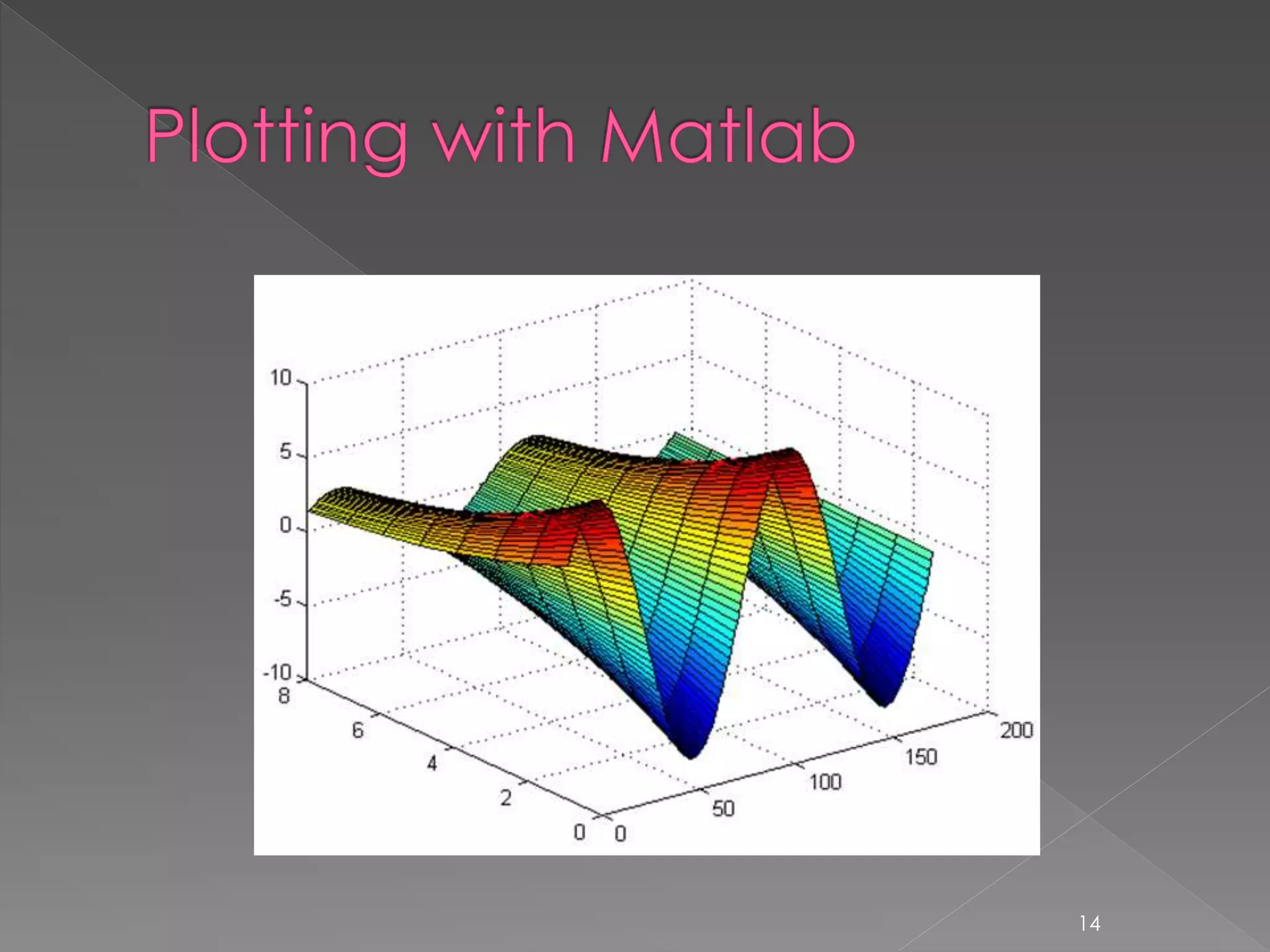
 Example:  >>> [x,y] = meshgrid(- 3:.1:3,-3:.1:3); >>> z = 3*(1-x).^2.*exp(- (x.^2) - (y+1).^2) ... - 10*(x/5 - x.^3 - y.^5).*exp(-x.^2-y.^2) ... - 1/3*exp(-(x+1).^2 - y.^2); >>> surf(z); 15

Graph Functions (summary)  Plot linear plot  stem discrete plot 16

 grid add grid lines  xlabel add X-axis label  ylabel add Y-axis label  title add graph title 17

 subplot divide figure window  figure create new figure window  pause wait for user response  hold on allows multiple plots on same axes  clf clears the figure window  axis([xmin,xmax,ymin,ymax]) controls axis properties 18

 Example: › plot(x,y,’r’) is a red line › plot(x,y,’o’) plots circles rather than lines › plot(x,y,’yp’) plots yellow pentagrams  Specialized 1D graphics › bar--bar chart › pie--pie chart › polar--polar coordintes › semilogy, semilogx, loglog—plotting with log- scales 20

Drawing a bar graph  >> clear, close all >> clc >> x = 0:pi/36:2*pi >> y = cos(x) >> bar(x,y,'b') 21

Drawing a stair-stop plot  >> clear, close all >> clc >> x = -10:0.5:10 >> y = x.^2 + 2.*x + 2 >> stairs(x,y,'b') 22

Elements of Matlab as a programming language: › Expressions: Arithmetic, logical, etc. › Flow Control blocks: Conditional and Iterations › Scripts › Functions 23

 When problems become complicated and require re– evaluation, entering command at MATLAB prompt is not practical  M-files are text files containing Matlab programs. Can be called form the command line or from other M-files 24

M-files: Scripts  Without input arguments, they do not return any value. 25

 To run the M-file, type in the name of the file at the prompt e.g. >>> test1  It will be executed provided that the saved file is in the known path  Type in matlabpath to check the list of directories listed in the path  Use path editor to add the path: File --> Set path … 26

M-files: Functions  Function is a ‘black box’ that communicates with workspace through input and output variables. 27

M-files: Functions  With parameters and returning values  Only visible variables defined inside the function or Parameters  Usually one file for each function defined  File must be saved to a known path with filename the same as the function name and with an extension ‘.m’  Call function by its name and arguments 28

 Write a script/function that converts a Roman numeral to its decimal equivalent.  You should be able to handle the following conversion table:  It will be useful to get the Roman number into your program as a string

 Matrix operators in Matlab are much faster than loops. Fast Matlab code uses * and avoids loops  Use built-in functions as they are often heavily optimized  Minimize division – x/2 takes longer than 0.5*x  Do computations outside loop  Pre-allocate arrays for j=1:n;a(j)=<something>;end Setting a=zeros(1,n) before the loop speeds things up  Use subfunctions file fname.m: function O=fname(I) function O2=fname2(I2) 31

 http://www.cs.cornell.edu/Courses/cs401/2001fa › Contains syllabus, lecture notes, examples, homework  http://www.mathworks.com/matlabcentral/ 32

 Advanced data objects (cell-arrays and structs)  Special tool boxes  Simulink  Graphical User Interface 33

Introduction to matlab lecture 4 of 4

More Related Content

What's hot

Viewers also liked

Similar to Introduction to matlab lecture 4 of 4

More from Randa Elanwar

Recently uploaded

Introduction to matlab lecture 4 of 4