This document provides an overview of optimization techniques that can be performed using MATLAB. It discusses unconstrained optimization problems where the goal is to minimize or maximize an objective function without any constraints on the variables. Constrained optimization problems are also discussed, where the goal is to optimize the objective function subject to certain equality and inequality constraints. MATLAB functions like fminsearch and fmincon can be used to find the optimal solution for unconstrained and constrained problems respectively. Gradient-based methods for solving constrained optimization problems are also briefly covered.
Overview of MATLAB's utility and basic interface components like Command Window and Workspace.
Introduction to defining and manipulating matrices including creation and subscripting.
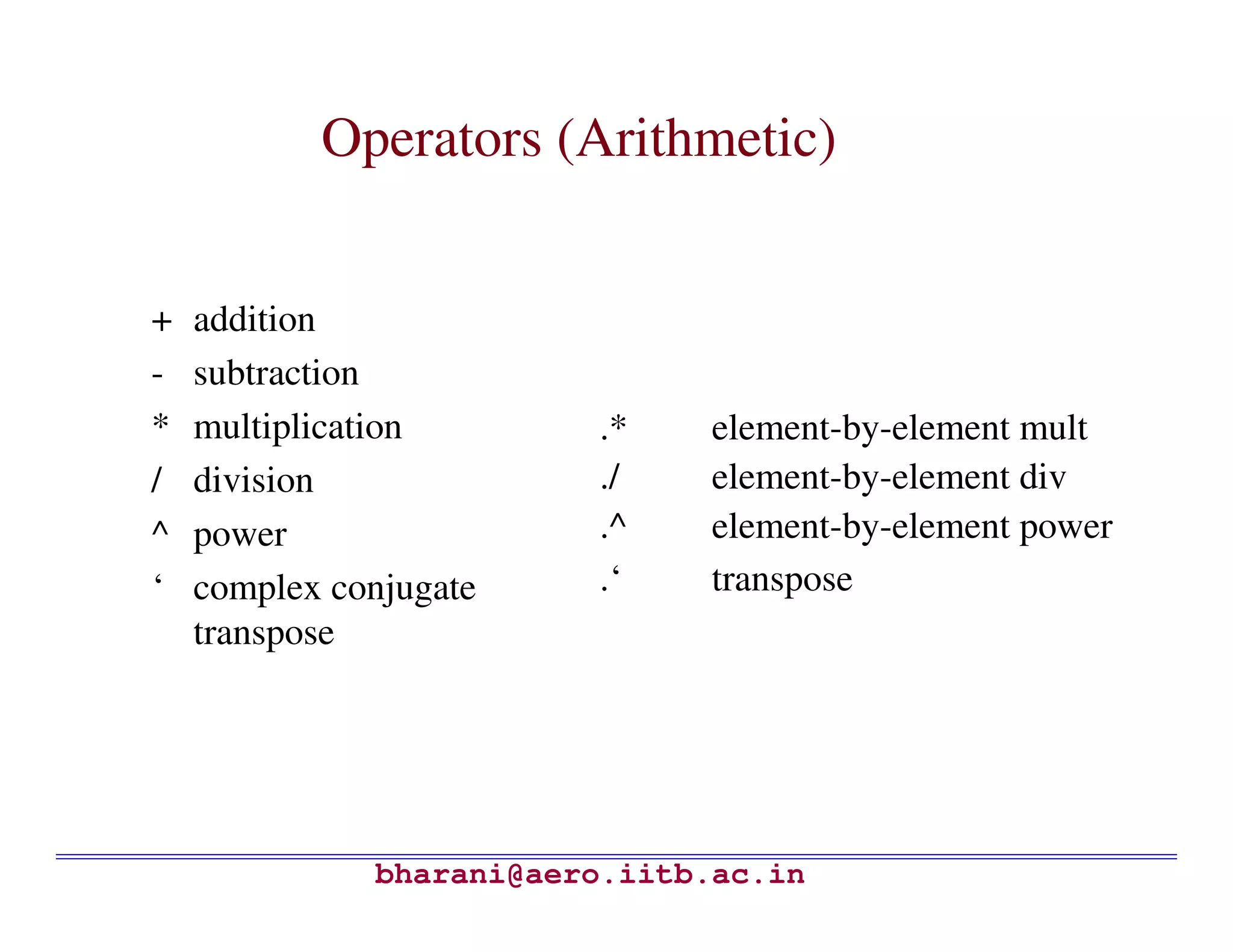
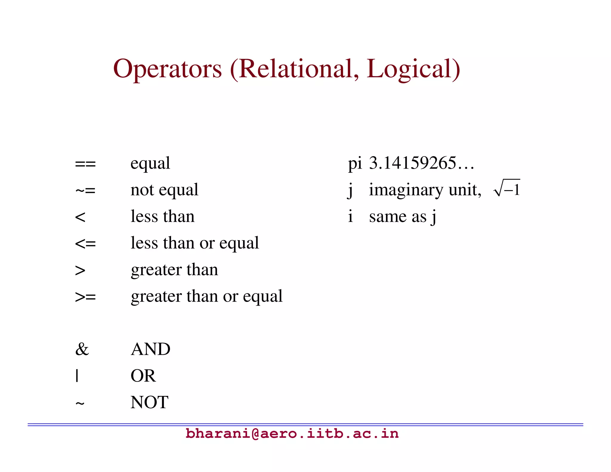
Overview of various operators in MATLAB such as arithmetic, relational, and logical operators.
Demonstrates matrix operations including determinants, eigenvalues, and matrix inversion in MATLAB.
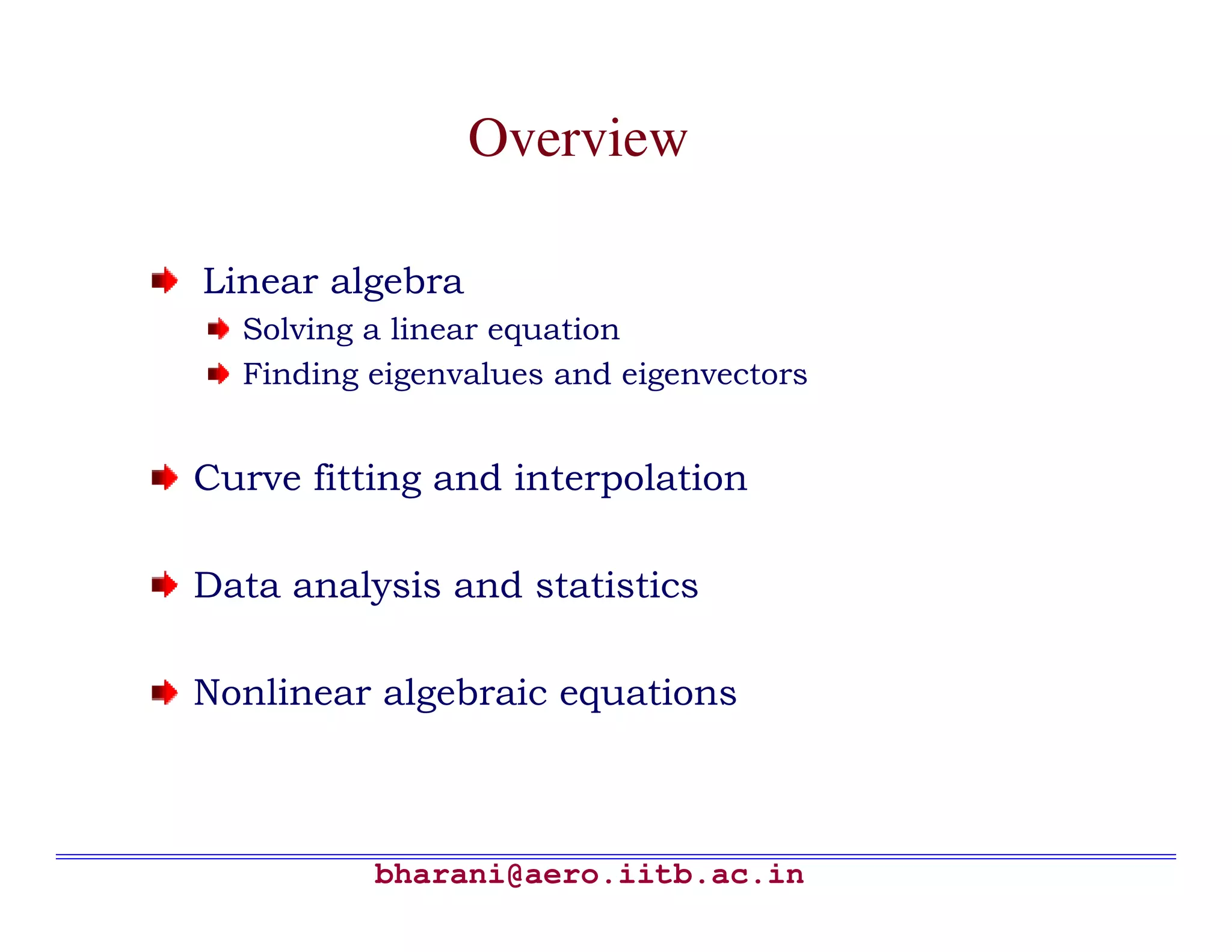
Applications of MATLAB in linear algebra, data analysis, curve fitting, and solving equations.
Tutorial on solving linear systems, finding eigenvalues and eigenvectors using MATLAB.
Explanation of curve fitting methods, plotting data points, and analyzing best-fit curves.
Differentiates between interpolation and curve fitting. Details MATLAB functions for interpolation.
Describes data analysis tasks like calculating mean, median, and statistics using MATLAB commands.Effective methods for solving nonlinear equations in MATLAB, including function definitions.
Discusses optimization importance in engineering and historical perspectives on optimization.
Uses of FMINCON for constrained optimization problems with clarification on its function.
Example problem illustrating how MATLAB's fminunc function finds local minima.
Detailed steps for solving constrained optimization problems using MATLAB.
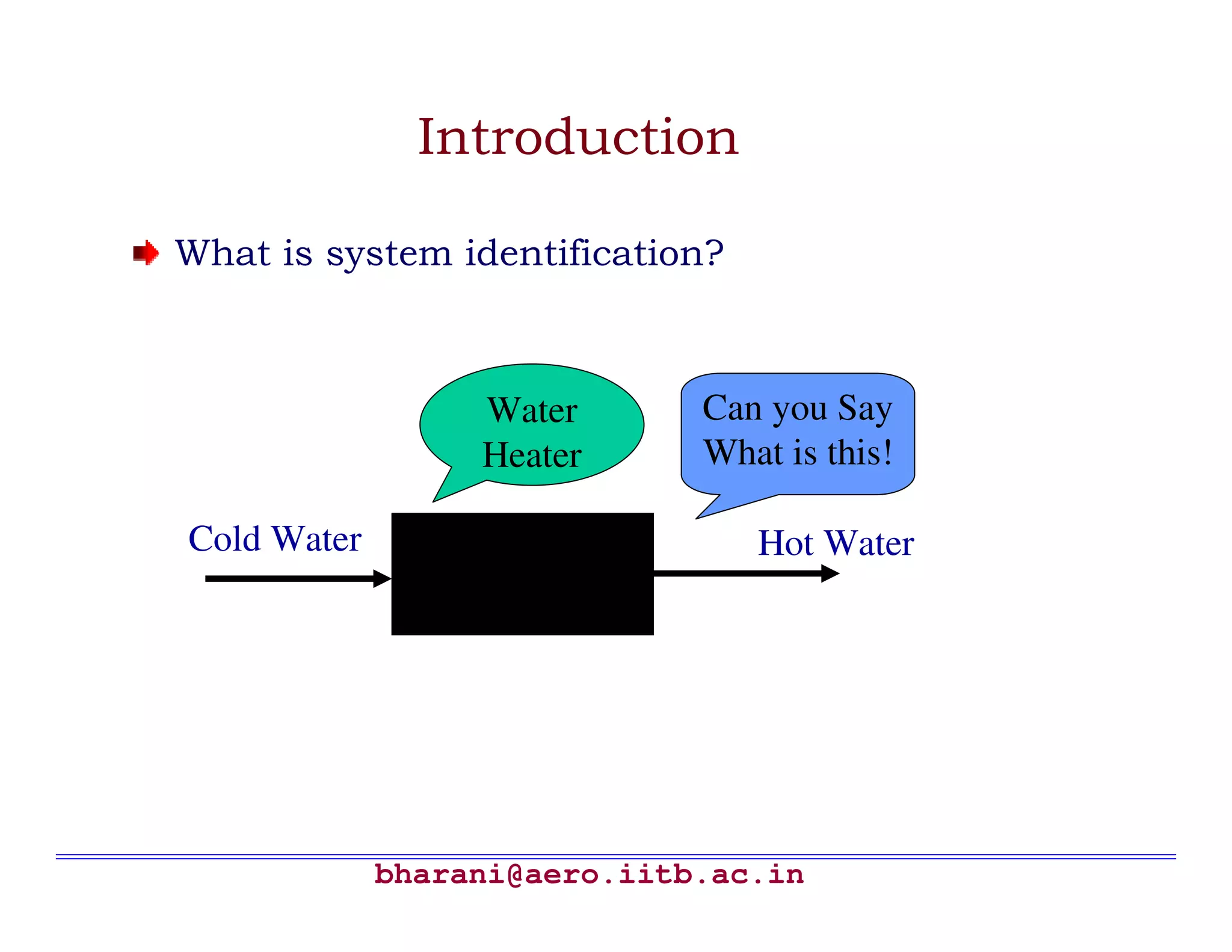
Introduction to system identification and its significance in modeling dynamic systems.
Basic steps in data handling and model estimation using MATLAB, including preprocessing.
Describes symbolic solving of ordinary differential equations with examples using dsolve.
Introduction to programming in MATLAB, discussion of M-files and decision-making structures.
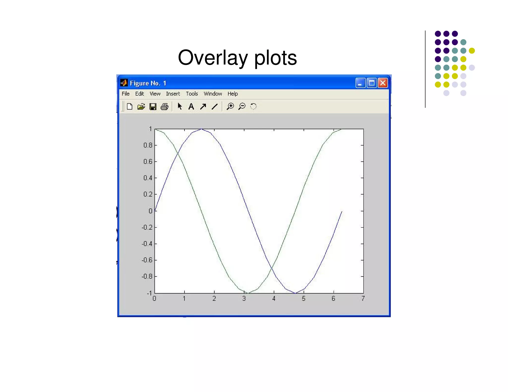
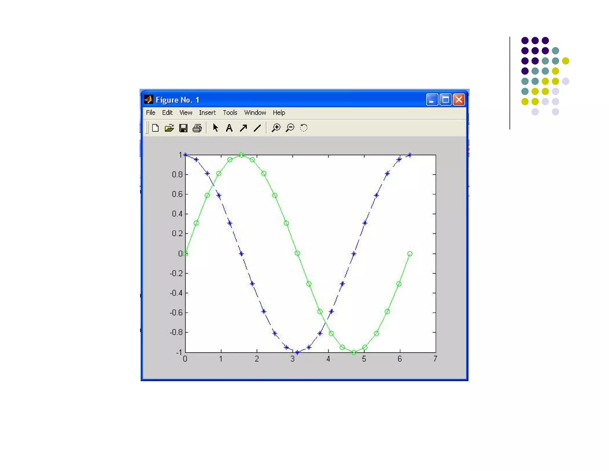
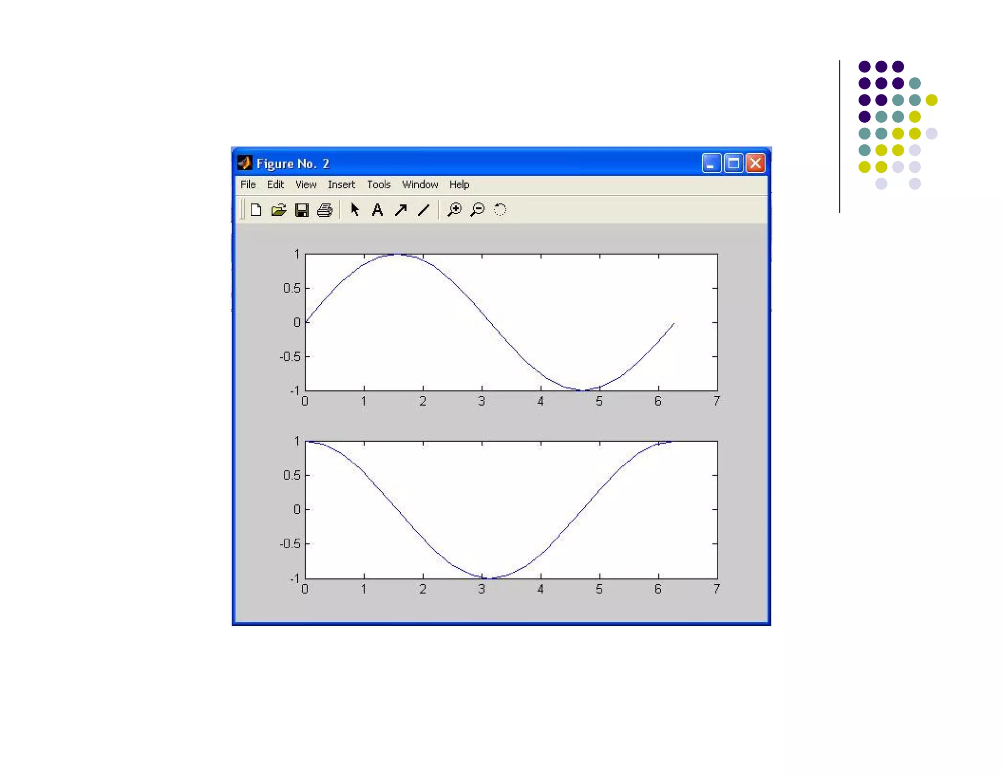
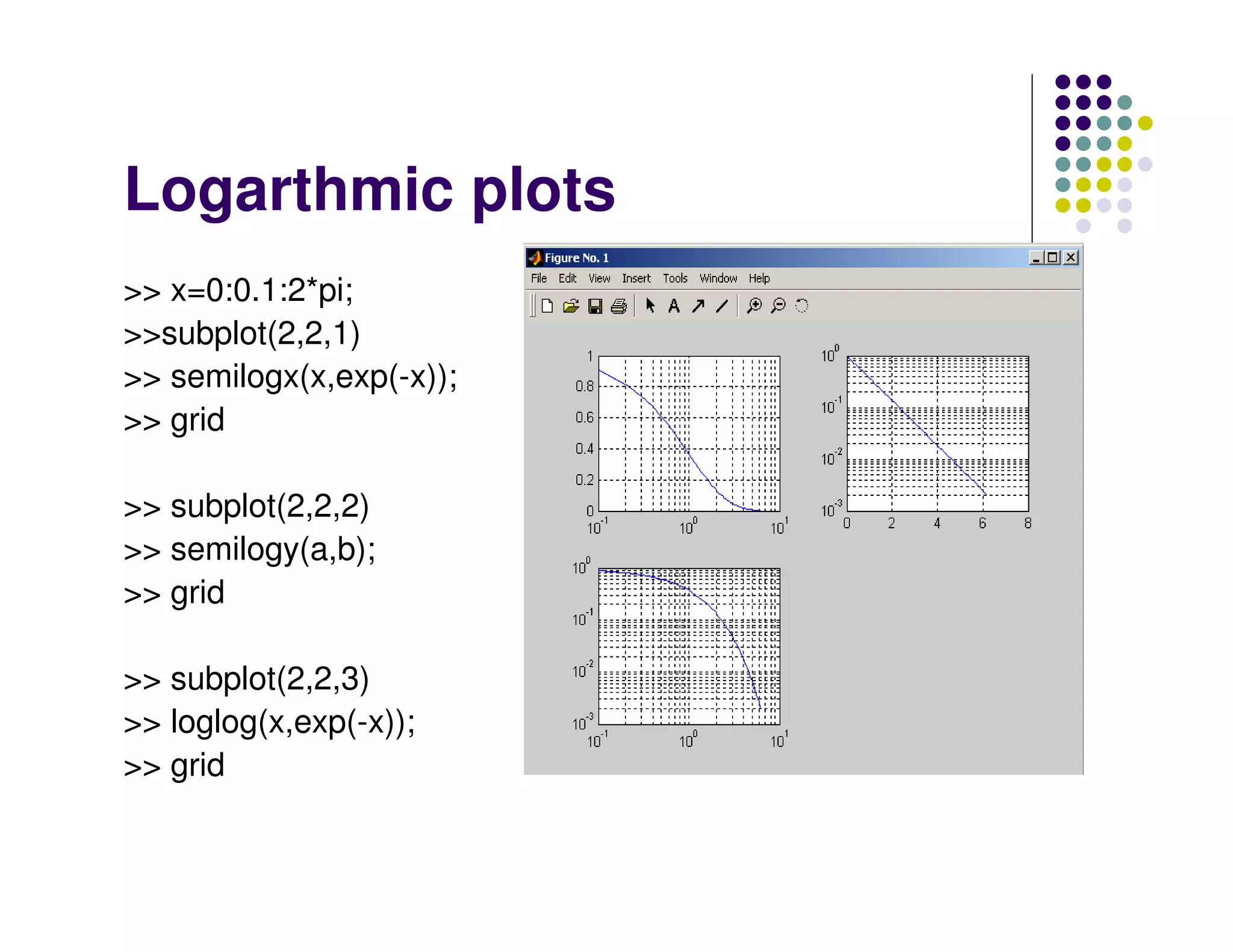
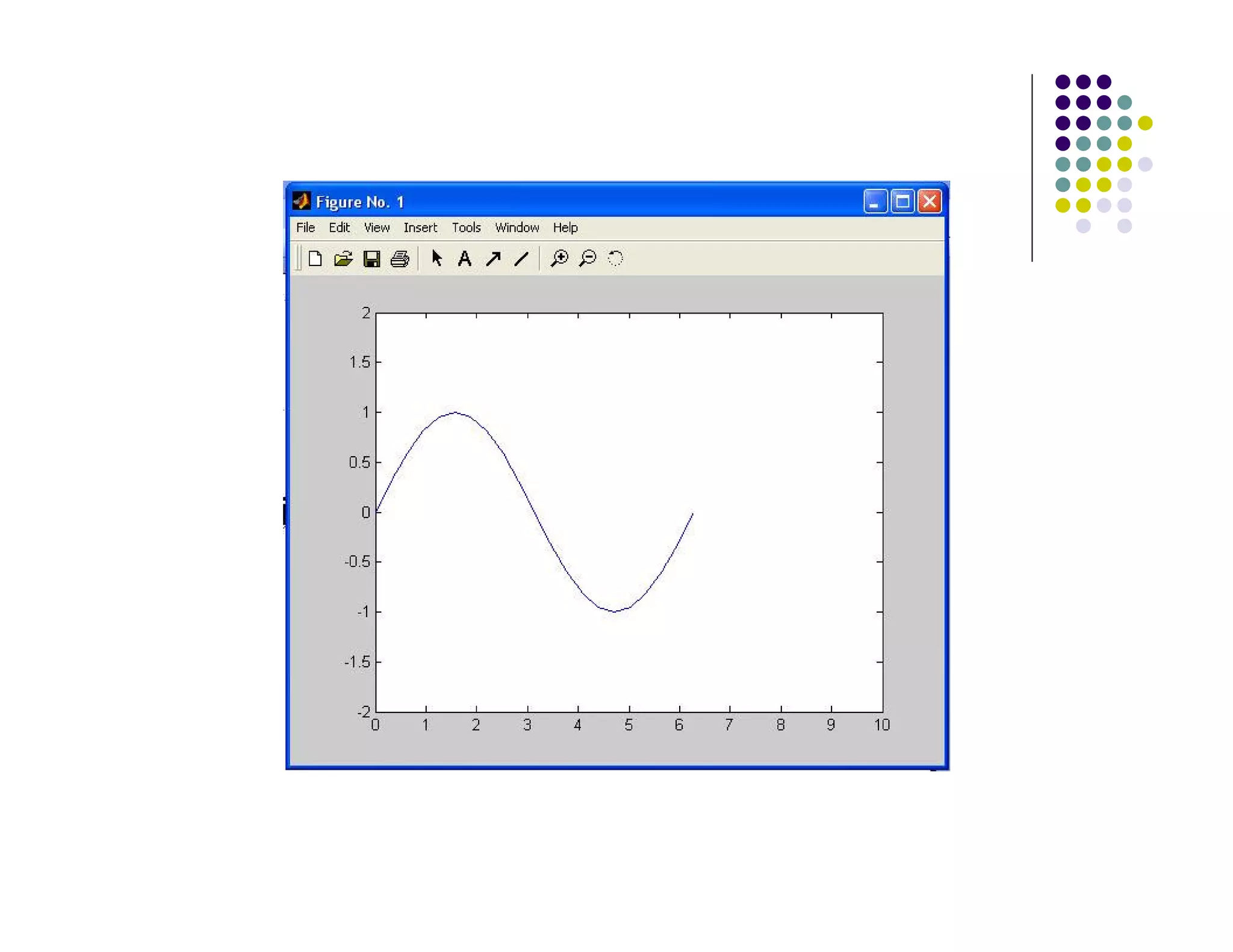
Basics of creating 2D plots, label adding, and using the plot editor in MATLAB.
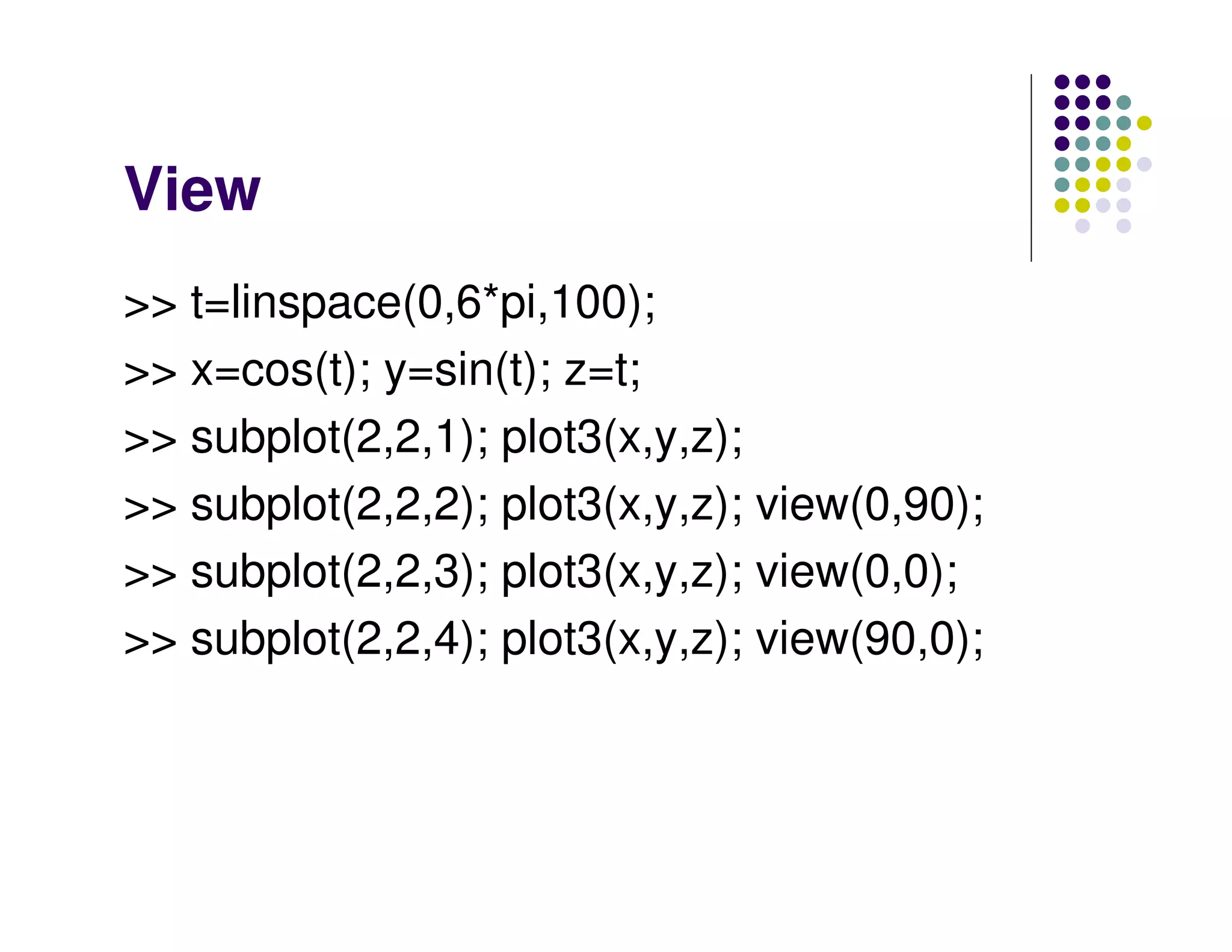
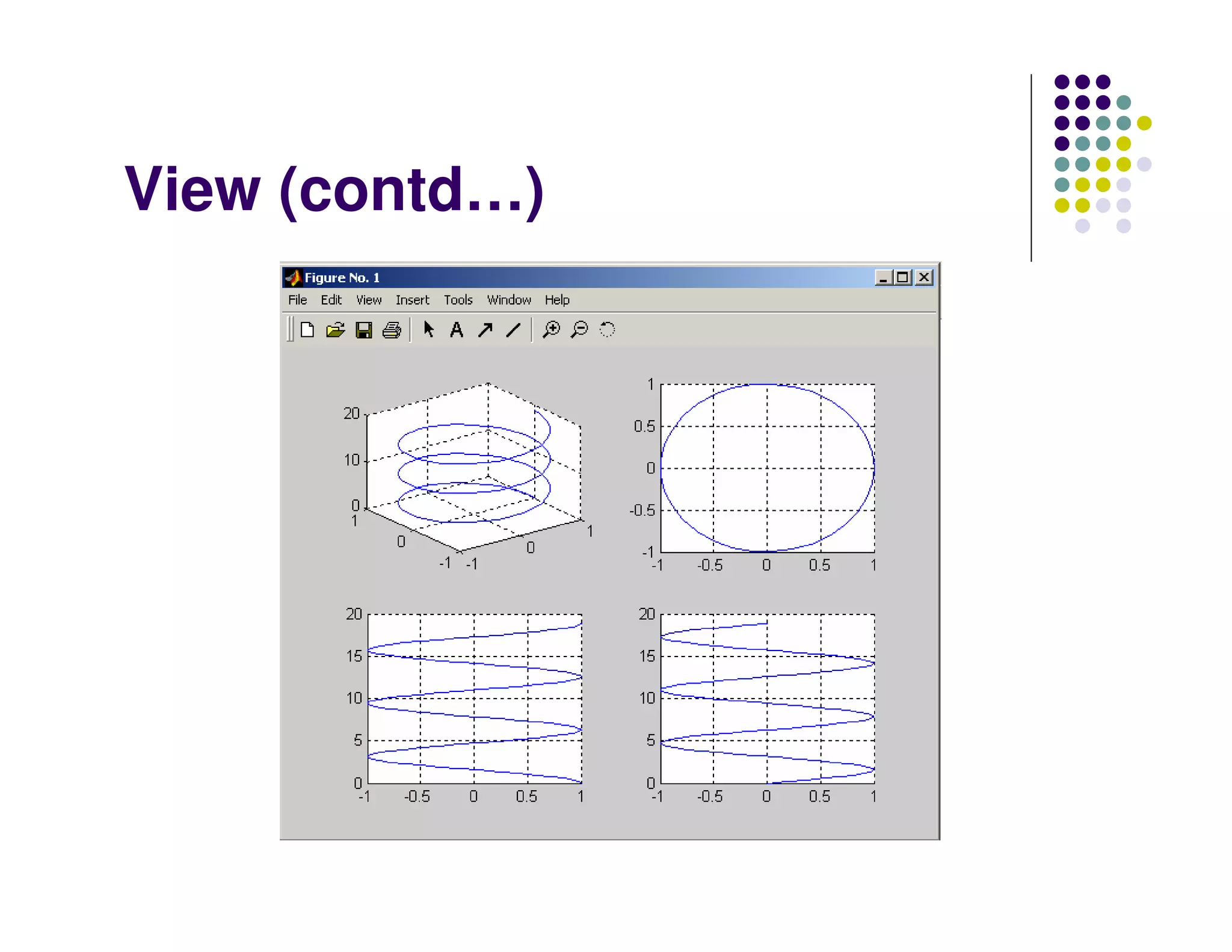
Introduction to 3D plotting, including mesh and surface plots to visualize functions.
Overview of MATLAB's handle graphics, including getting and setting properties of graphics objects.
bharani@aero.iitb.ac.in Desktop Tools Command Window typecommands Workspace view program variables clear to clear double click on a variable to see it in the Array Editor Command History view past commands save a whole session using diary
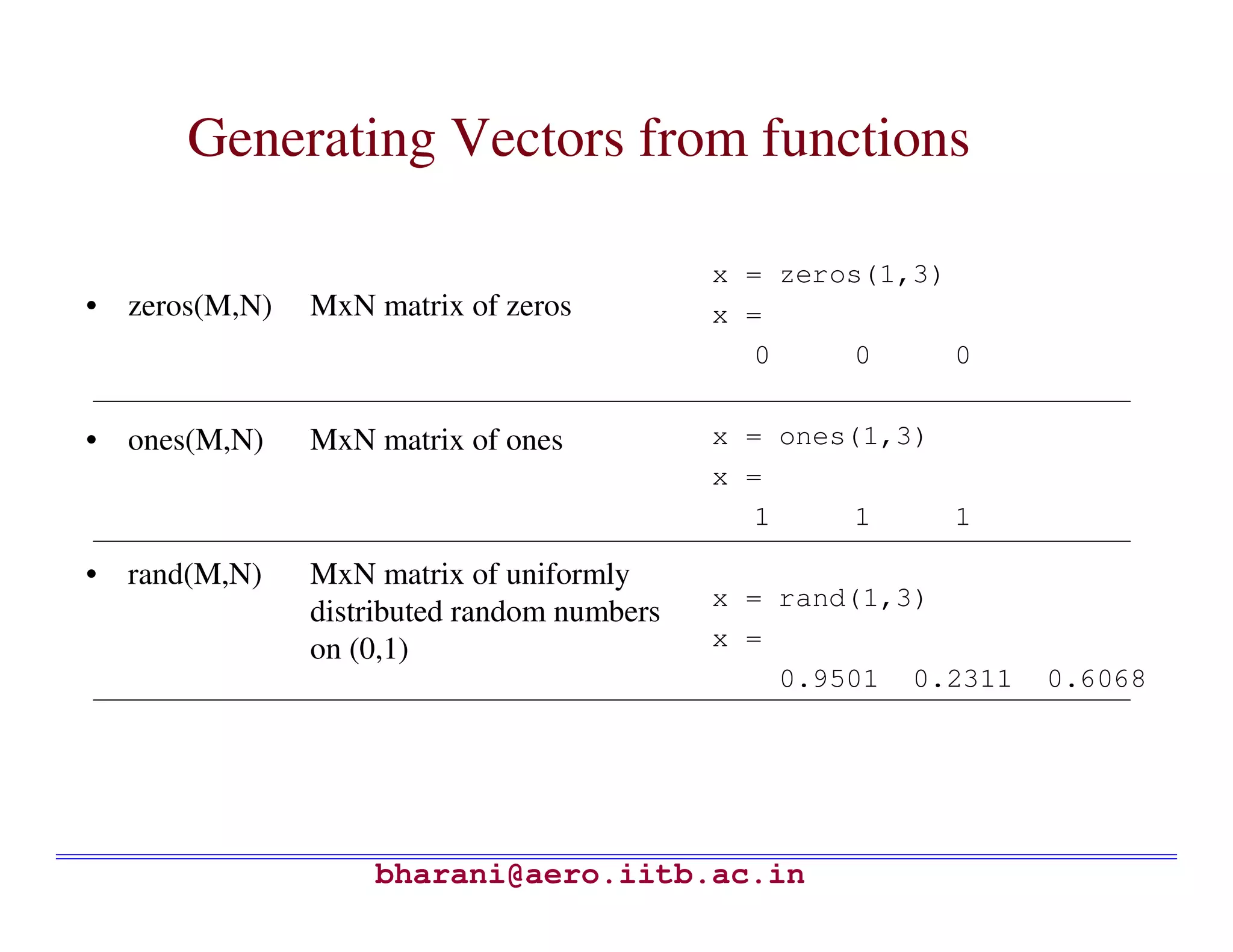
bharani@aero.iitb.ac.in Generating Vectors fromfunctions • zeros(M,N) MxN matrix of zeros • ones(M,N) MxN matrix of ones • rand(M,N) MxN matrix of uniformly distributed random numbers on (0,1) x = zeros(1,3) x = 0 0 0 x = ones(1,3) x = 1 1 1 x = rand(1,3) x = 0.9501 0.2311 0.6068
bharani@aero.iitb.ac.in Linear Algebra Solving alinear system Find the values of x, y and z for the following equations: 5x = 3y – 2z +10 8y +4z = 3x + 20 2x + 4y - 9z = 9 Step 1: Rearrange equations: 5x - 3y + 2z = 10 - 3x + 8y +4z = 20 2x + 4y - 9z = 9 Step 2: Write the equations in matrix form: [A] x = b − − − = 942 483 235 A = 9 20 10 b
16.
bharani@aero.iitb.ac.in Linear Algebra (Contd…) Step3: Solve the matrix equation in MATLAB: >> A = [ 5 -3 2; -3 8 4; 2 4 -9]; >> b = [10; 20; 9] >> x = A b x = 3.442 3.1982 1.1868 % Veification >> c = A*x >> c = 10.0000 20.0000 9.0000
17.
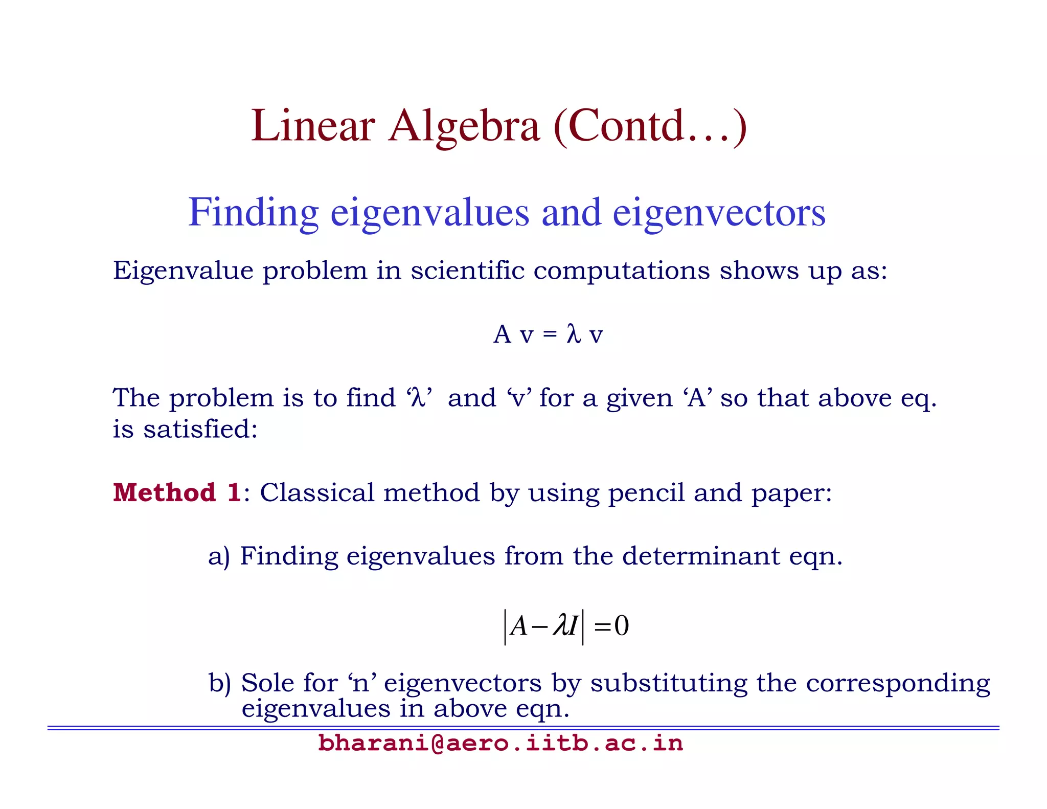
bharani@aero.iitb.ac.in Finding eigenvalues andeigenvectors Eigenvalue problem in scientific computations shows up as: A v = λ v The problem is to find ‘λ’ and ‘v’ for a given ‘A’ so that above eq. is satisfied: Method 1: Classical method by using pencil and paper: a) Finding eigenvalues from the determinant eqn. b) Sole for ‘n’ eigenvectors by substituting the corresponding eigenvalues in above eqn. 0=− IA λ Linear Algebra (Contd…)
18.
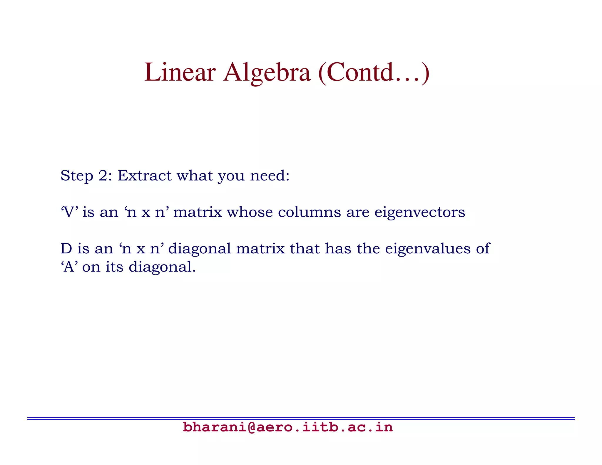
bharani@aero.iitb.ac.in Method 2: Byusing MATLAB: Step 1: Enter matrix A and type [V, D] = eig(A) >> A = [ 5 -3 2; -3 8 4; 2 4 -9]; >> [V, D] = eig(A) V = -0.1709 0.8729 0.4570 -0.2365 0.4139 -0.8791 0.9565 0.2583 -0.1357 D = -10.3463 0 0 0 4.1693 0 0 0 10.1770 Linear Algebra (Contd…)
19.
bharani@aero.iitb.ac.in Step 2: Extractwhat you need: ‘V’ is an ‘n x n’ matrix whose columns are eigenvectors D is an ‘n x n’ diagonal matrix that has the eigenvalues of ‘A’ on its diagonal. Linear Algebra (Contd…)
20.
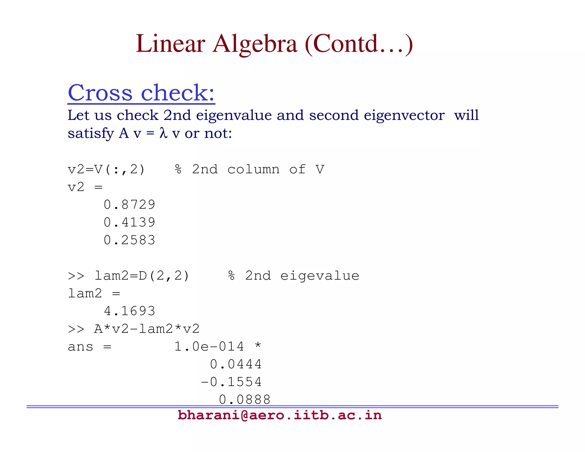
bharani@aero.iitb.ac.in Cross check: Let uscheck 2nd eigenvalue and second eigenvector will satisfy A v = λ v or not: v2=V(:,2) % 2nd column of V v2 = 0.8729 0.4139 0.2583 >> lam2=D(2,2) % 2nd eigevalue lam2 = 4.1693 >> A*v2-lam2*v2 ans = 1.0e-014 * 0.0444 -0.1554 0.0888 Linear Algebra (Contd…)
21.
bharani@aero.iitb.ac.in Curve Fitting What iscurve fitting ? It is a technique of finding an algebraic relationship that “best” fits a given set of data. There is no magical function that can give you this relationship. You have to have an idea of what kind of relationship might exist between the input data (x) and output data (y). If you do not have a firm idea but you have data that you trust, MATLAB can help you to explore the best possible fit.
22.
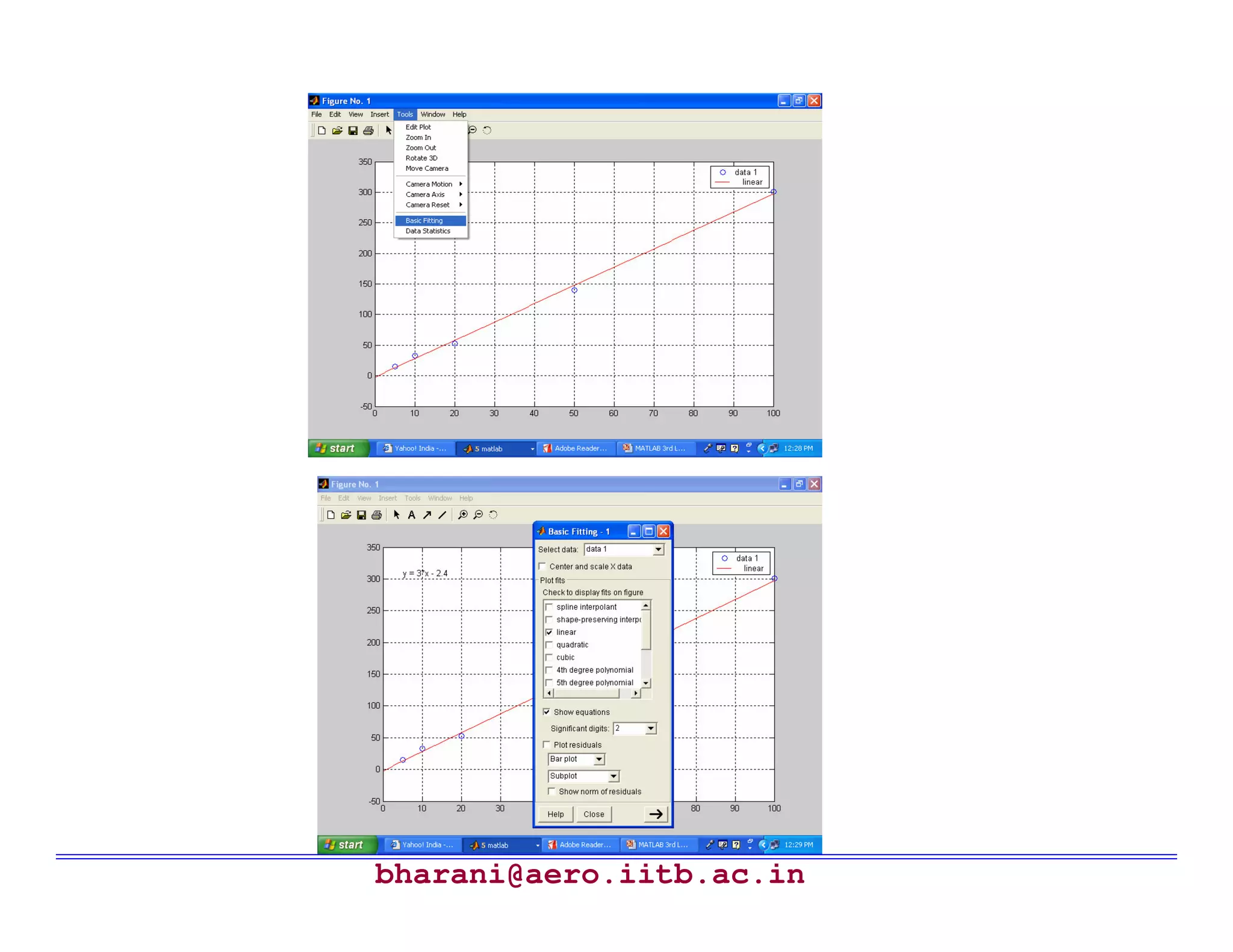
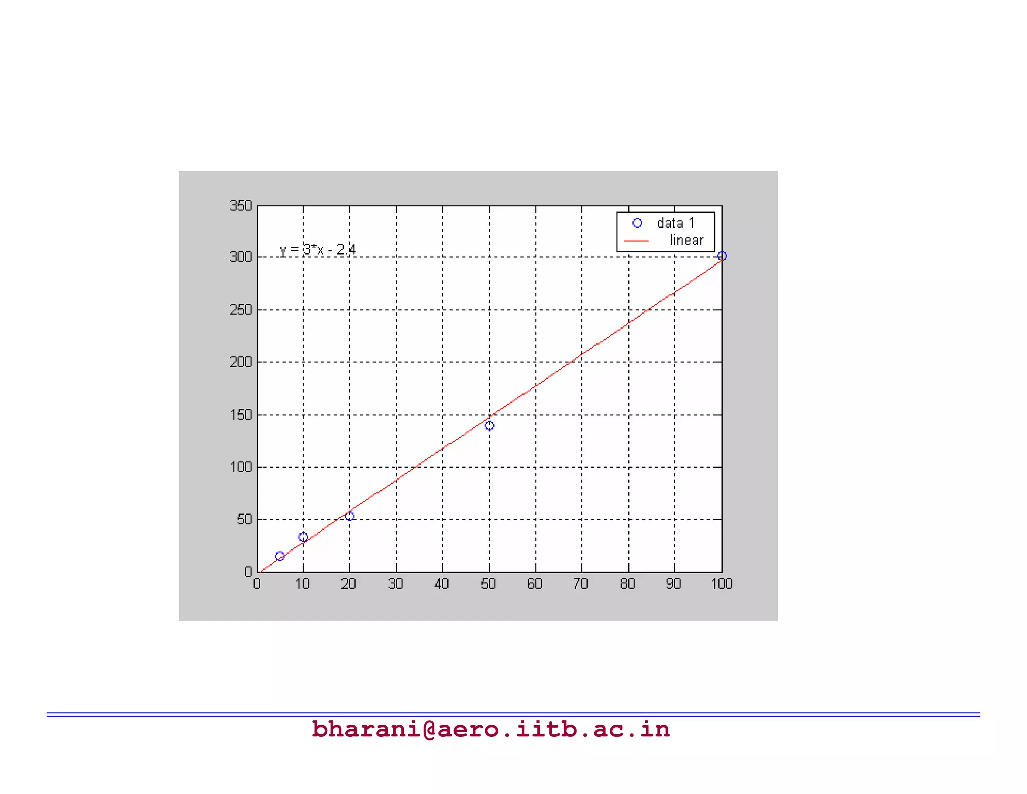
bharani@aero.iitb.ac.in Curve Fitting (Contd…) Example1 : straight line (linear) fit: Step 1: Plot raw data: Enter the data in MATLAB and plot it: >> x = [ 5 10 20 50 100]; >> y = [15 33 53 140 301]; >> plot (x,y,’o’) >> grid 301140533315Y 1005020105x
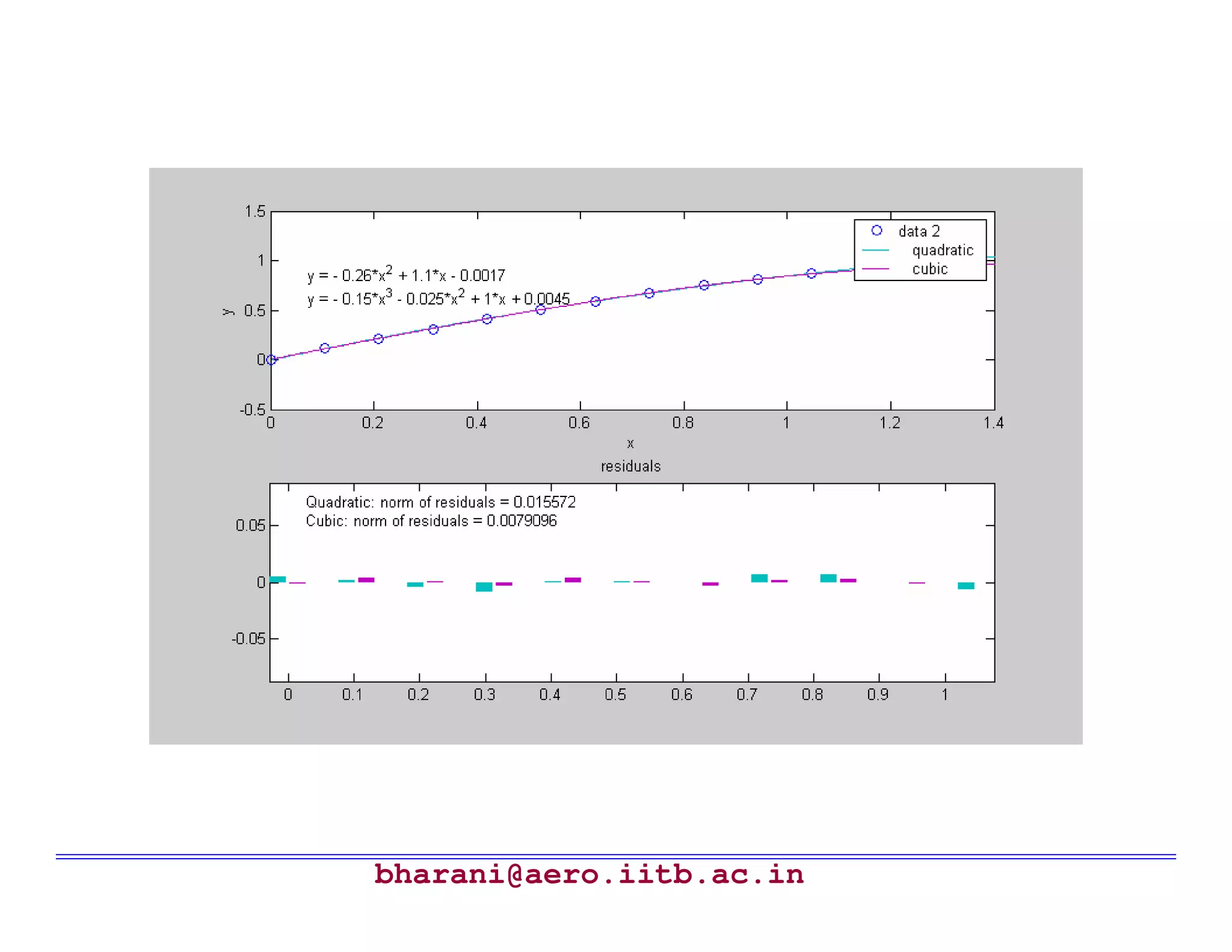
bharani@aero.iitb.ac.in Curve Fitting (Contd…) Example2 : Comparing different fits: x = 0: pi/30 : pi/3 y = sin(x) + rand (size(x))/100 Step 1: Plot raw data: >> plot (x,y,’o’) >> grid Step 2: Use basic fitting to do a quadratic and cubic fit Step 3 : Choose the best fit based on the residuals
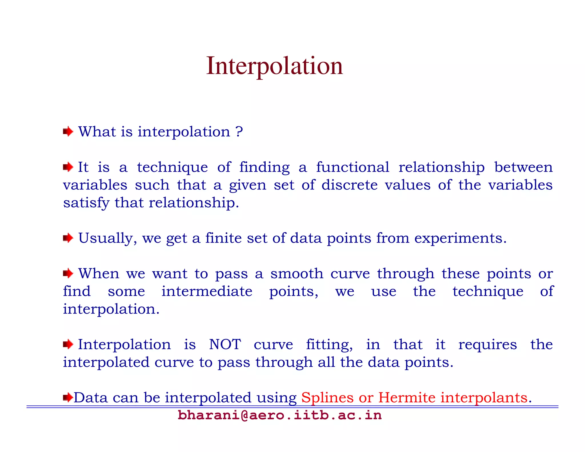
bharani@aero.iitb.ac.in Interpolation What is interpolation? It is a technique of finding a functional relationship between variables such that a given set of discrete values of the variables satisfy that relationship. Usually, we get a finite set of data points from experiments. When we want to pass a smooth curve through these points or find some intermediate points, we use the technique of interpolation. Interpolation is NOT curve fitting, in that it requires the interpolated curve to pass through all the data points. Data can be interpolated using Splines or Hermite interpolants.
28.
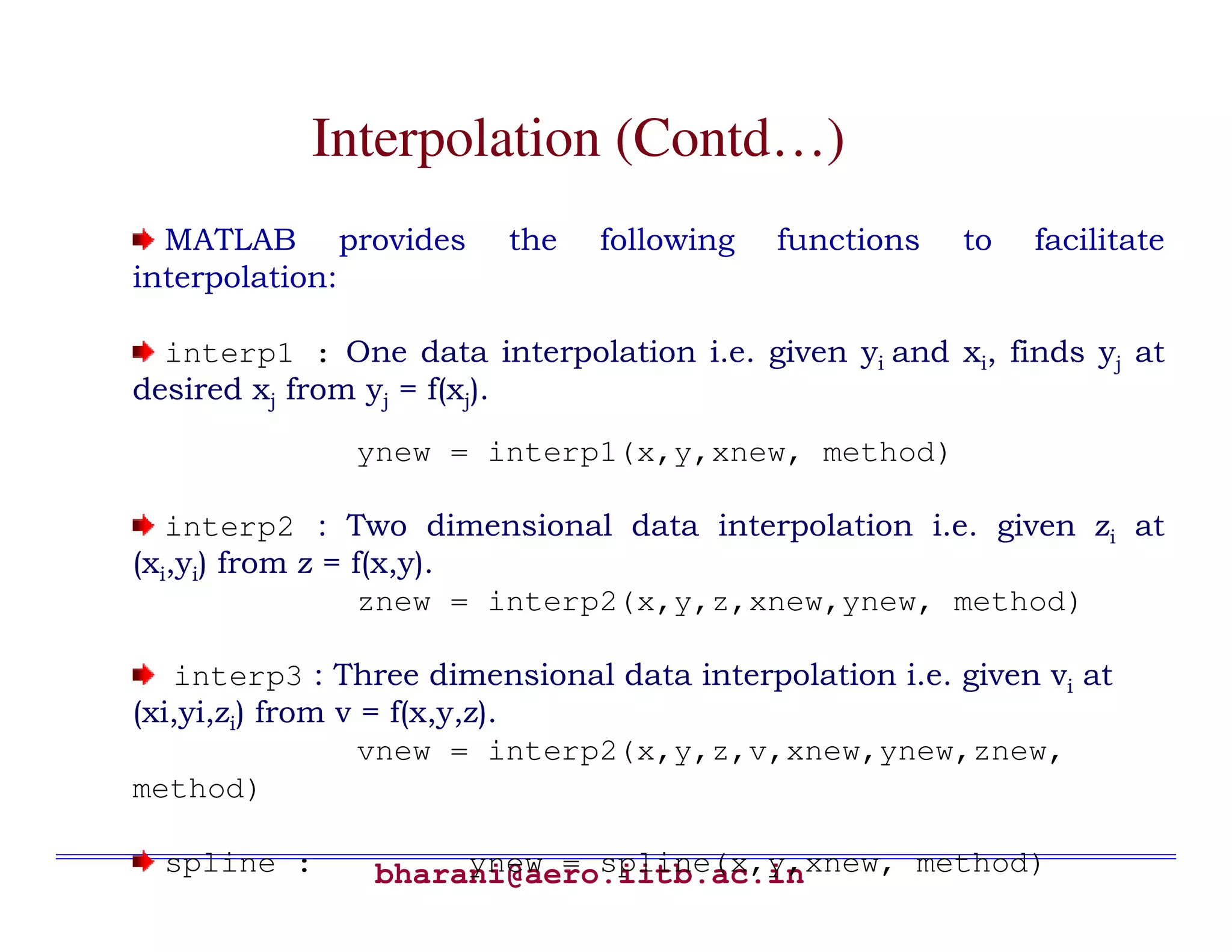
bharani@aero.iitb.ac.in Interpolation (Contd…) MATLAB providesthe following functions to facilitate interpolation: interp1 : One data interpolation i.e. given yi and xi, finds yj at desired xj from yj = f(xj). ynew = interp1(x,y,xnew, method) interp2 : Two dimensional data interpolation i.e. given zi at (xi,yi) from z = f(x,y). znew = interp2(x,y,z,xnew,ynew, method) interp3 : Three dimensional data interpolation i.e. given vi at (xi,yi,zi) from v = f(x,y,z). vnew = interp2(x,y,z,v,xnew,ynew,znew, method) spline : ynew = spline(x,y,xnew, method)
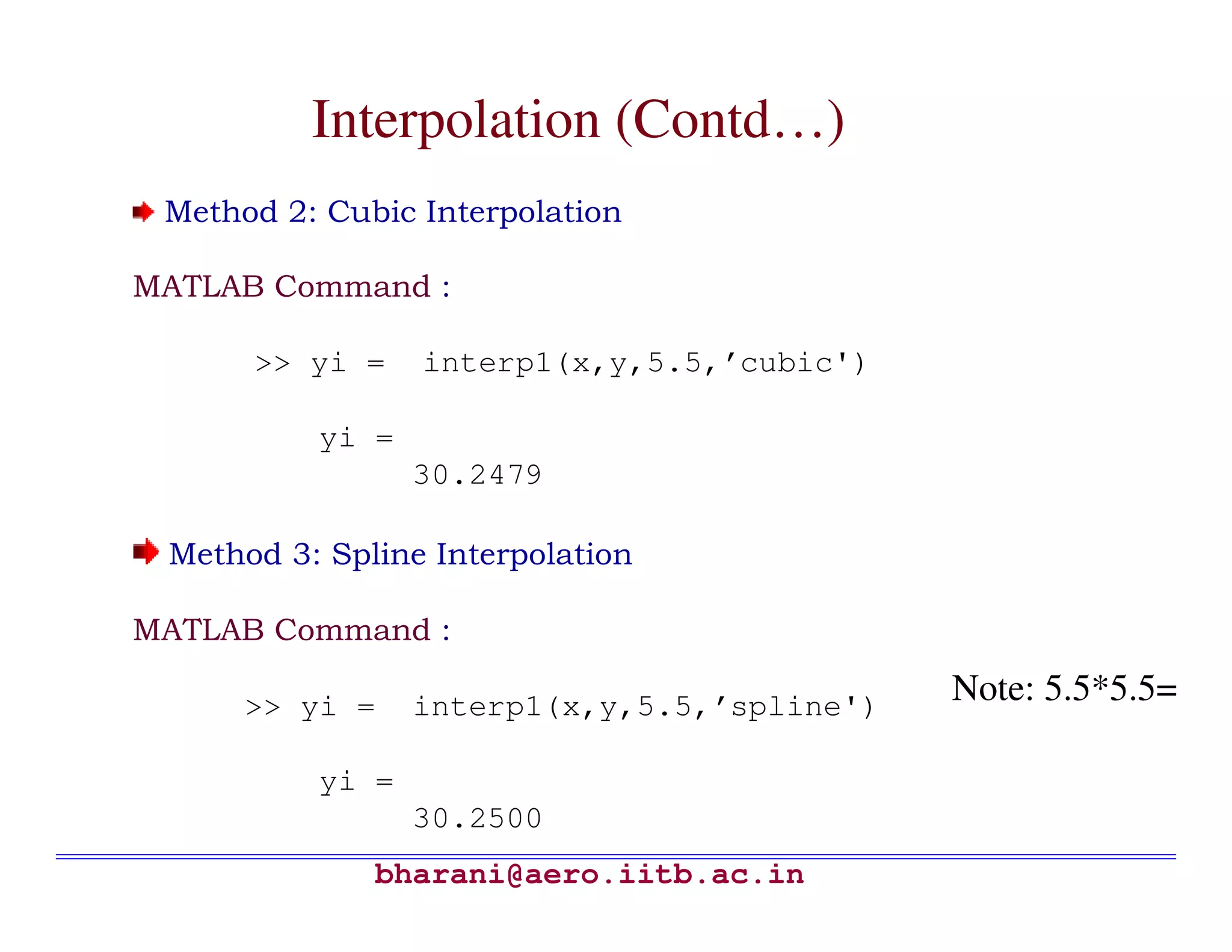
bharani@aero.iitb.ac.in Interpolation (Contd…) Method 2:Cubic Interpolation MATLAB Command : >> yi = interp1(x,y,5.5,’cubic') yi = 30.2479 Method 3: Spline Interpolation MATLAB Command : >> yi = interp1(x,y,5.5,’spline') yi = 30.2500 Note: 5.5*5.5=
31.
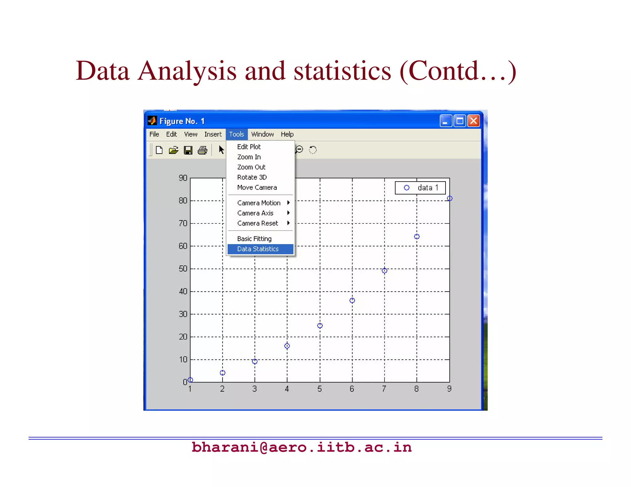
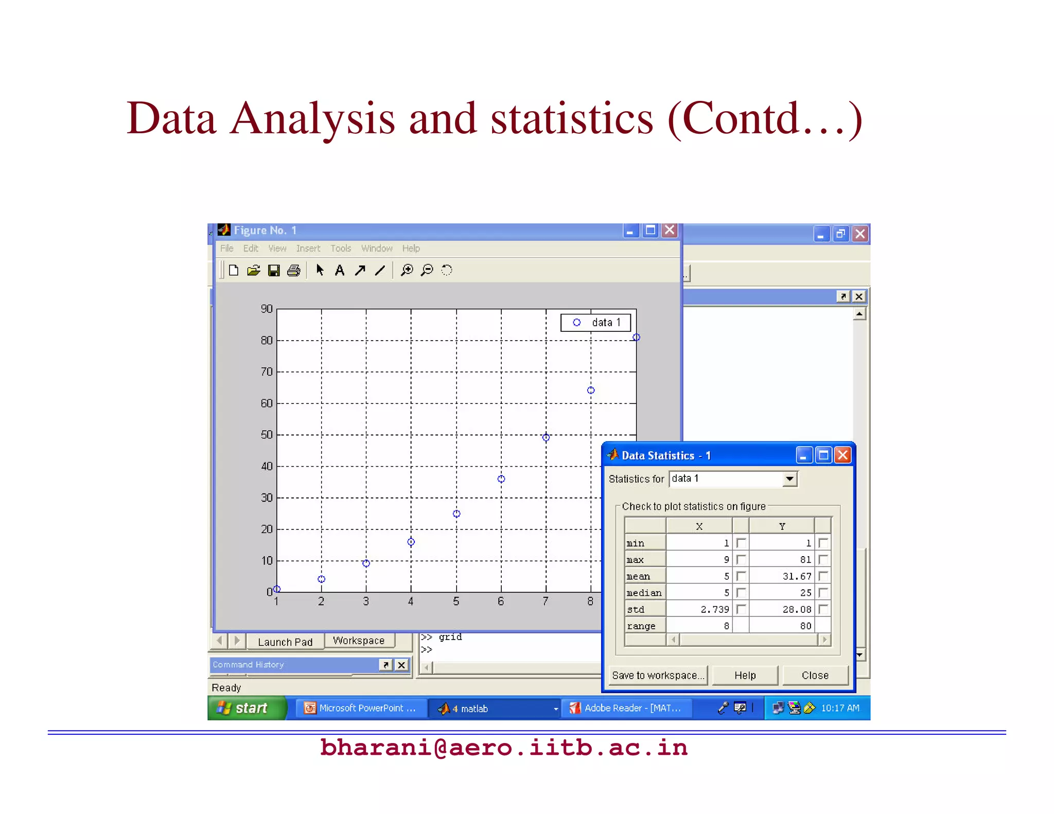
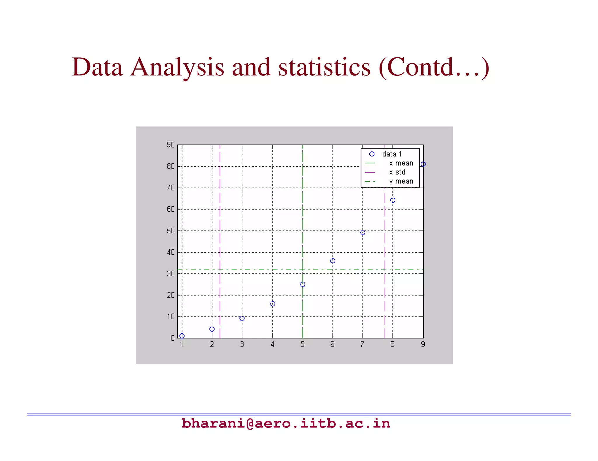
bharani@aero.iitb.ac.in Data Analysis andstatistics It includes various tasks, such as finding mean, median, standard deviation, etc. MATLAB provides an easy graphical interface to do such type of tasks. As a first step, you should plot your data in the form you wish. Then go to the figure window and select data statistics from the tools menu. Any of the statistical measures can be seen by checking the appropriate box.
32.
bharani@aero.iitb.ac.in Data Analysis andstatistics (Contd…) Example: x = [1 2 3 4 5 6 7 8 9] y = [1 4 9 16 25 36 49 64 81] Find the minimum value, maximum value, mean, median?
bharani@aero.iitb.ac.in Data Analysis andstatistics (Contd…) It can be performed directly by using MATLAB commands also: Consider: x = [1 2 3 4 5] mean (x) : Gives arithmetic mean of ‘x’ or the avg. data. MATLAB usage: mean (x) gives 3. median (x) : gives the middle value or arithmetic mean of two middle Numbers. MATLAB usage: median (x) gives 3. Std(x): gives the standard deviation Max(x)/min(x): gives the largest/smallest value
37.
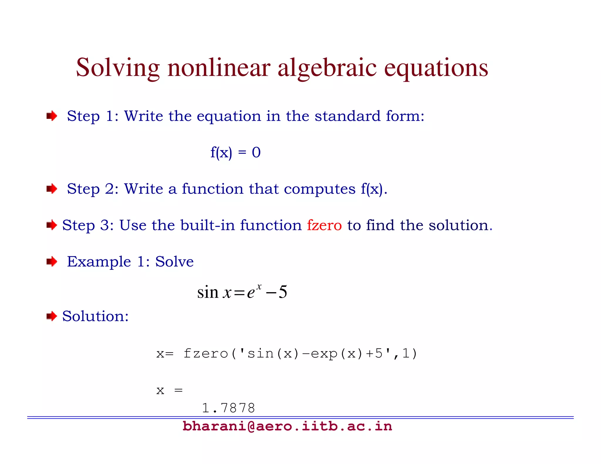
bharani@aero.iitb.ac.in Solving nonlinear algebraicequations Step 1: Write the equation in the standard form: f(x) = 0 Step 2: Write a function that computes f(x). Step 3: Use the built-in function fzero to find the solution. Example 1: Solve Solution: x= fzero('sin(x)-exp(x)+5',1) x = 1.7878 5sin −= x ex
bharani@aero.iitb.ac.in Why Optimize! Engineers arealways interested in finding the ‘best’ solution to the problem at hand Fastest Fuel Efficient Optimization theory allows engineers to accomplish this Often the solution may not be easily obtained In the past, it has been surrounded by certain mistakes
43.
bharani@aero.iitb.ac.in The Greeks startedit! Queen Dido of Carthage (7 century BC) – Daughter of the king of Tyre – Agreed to buy as much land as she could “enclose with one bull’s hide” – Set out to choose the largest amount of land possible, with one border along the sea • A semi-circle with side touching the ocean • Founded Carthage – Fell in love with Aeneas but committed suicide when he left.
44.
bharani@aero.iitb.ac.in The Italians Countered JosephLouis Lagrange (1736-1813) His work Mécanique Analytique (Analytical Mechanics) (1788) was a mathematical masterpiece Invented the method of ‘variations’ which impressed Euler and became ‘calculus of variations’ Invented the method of multipliers (Lagrange multipliers) Sensitivities of the performance index to changes in states/constraints Became the ‘father’ of ‘Lagrangian’ Dynamics Euler-Lagrange Equations
45.
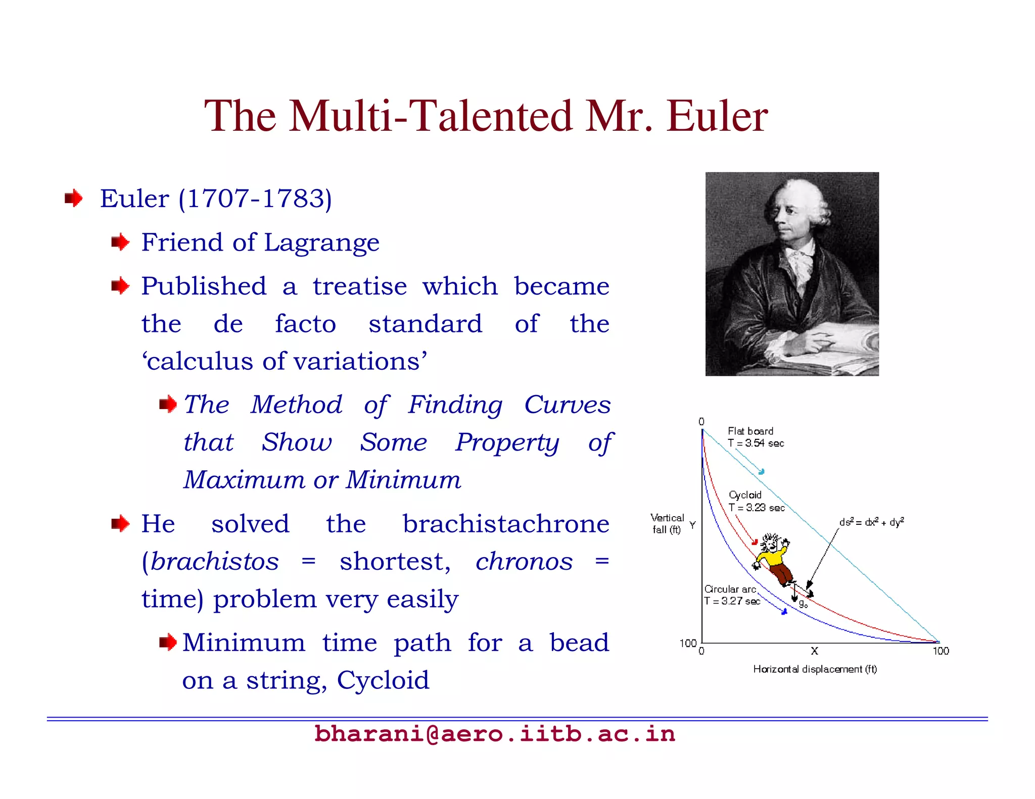
bharani@aero.iitb.ac.in The Multi-Talented Mr.Euler Euler (1707-1783) Friend of Lagrange Published a treatise which became the de facto standard of the ‘calculus of variations’ The Method of Finding Curves that Show Some Property of Maximum or Minimum He solved the brachistachrone (brachistos = shortest, chronos = time) problem very easily Minimum time path for a bead on a string, Cycloid
46.
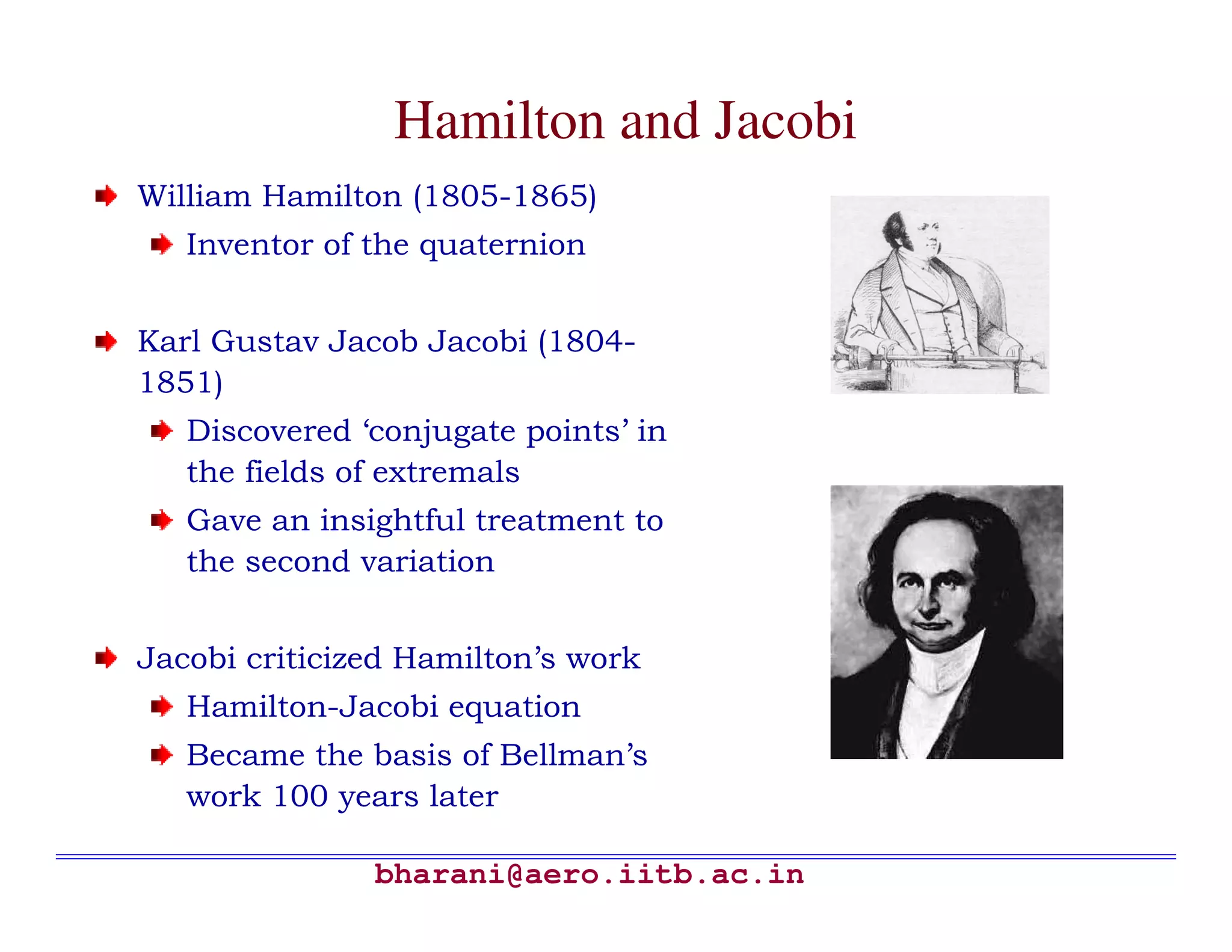
bharani@aero.iitb.ac.in Hamilton and Jacobi WilliamHamilton (1805-1865) Inventor of the quaternion Karl Gustav Jacob Jacobi (1804- 1851) Discovered ‘conjugate points’ in the fields of extremals Gave an insightful treatment to the second variation Jacobi criticized Hamilton’s work Hamilton-Jacobi equation Became the basis of Bellman’s work 100 years later
47.
bharani@aero.iitb.ac.in What to Optimize? Engineersintuitively know what they are interested in optimizing Straightforward problems Fuel Time Power Effort More complex Maximum margin Minimum risk The mathematical quantity we optimize is called a cost function or performance index
48.
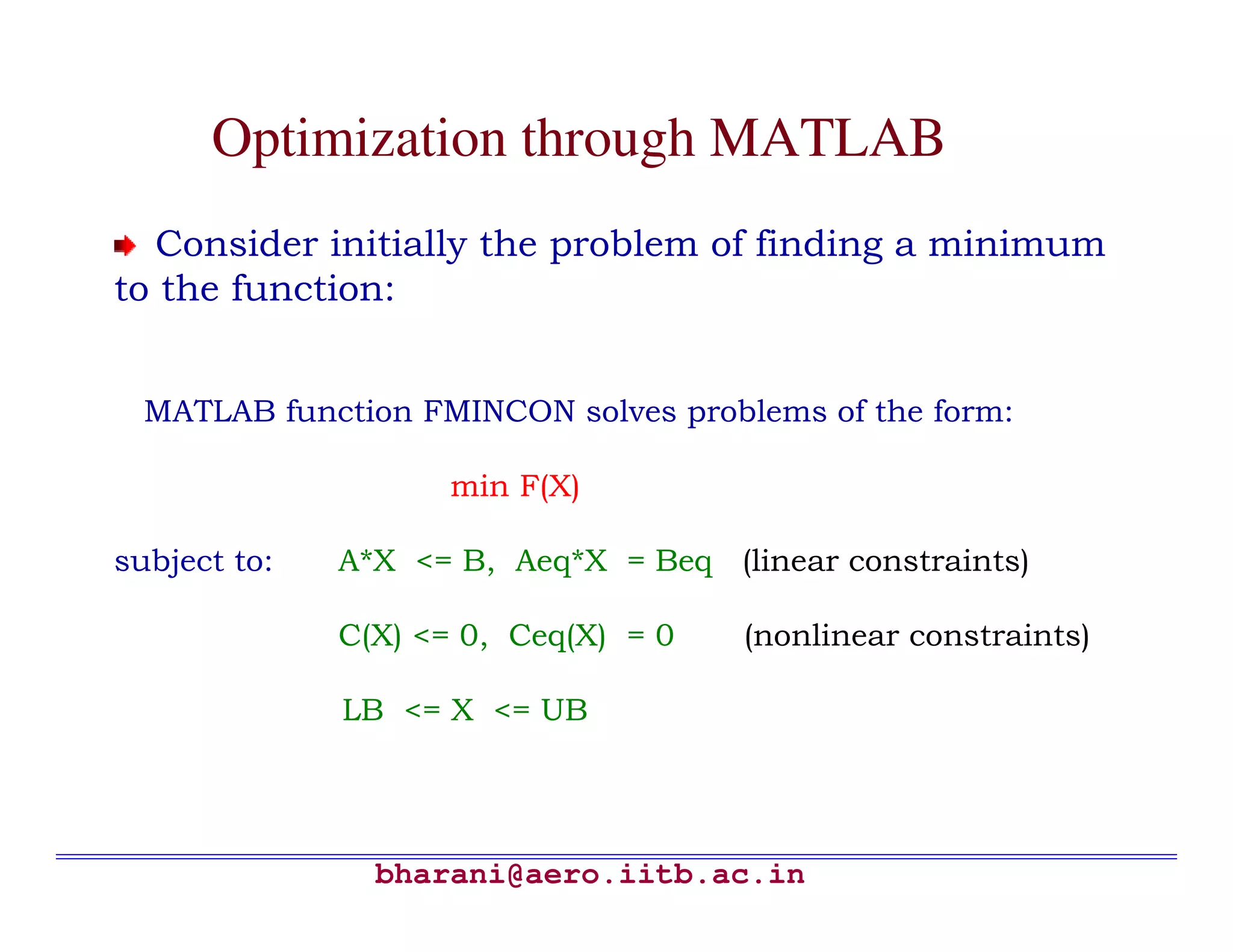
bharani@aero.iitb.ac.in Optimization through MATLAB Considerinitially the problem of finding a minimum to the function: MATLAB function FMINCON solves problems of the form: min F(X) subject to: A*X <= B, Aeq*X = Beq (linear constraints) C(X) <= 0, Ceq(X) = 0 (nonlinear constraints) LB <= X <= UB
49.
bharani@aero.iitb.ac.in X = FMINCON(FUN,X0,A,B)starts at X0 and finds a minimum X to the function FUN, subject to the linear inequalities A*X <= B. X=FMINCON(FUN,X0,A,B,Aeq,Beq) minimizes FUN subject to the linear equalities: Aeq*X = Beq as well as A*X <= B. (Set A=[ ] and B=[ ] if no inequalities exist.) Optimization through MATLAB (Contd…)
50.
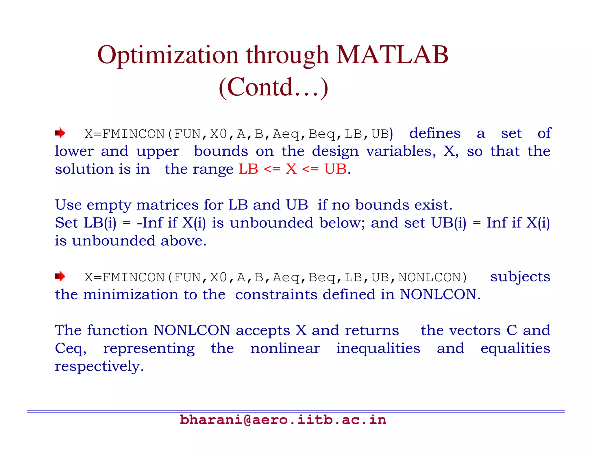
bharani@aero.iitb.ac.in X=FMINCON(FUN,X0,A,B,Aeq,Beq,LB,UB) defines aset of lower and upper bounds on the design variables, X, so that the solution is in the range LB <= X <= UB. Use empty matrices for LB and UB if no bounds exist. Set LB(i) = -Inf if X(i) is unbounded below; and set UB(i) = Inf if X(i) is unbounded above. X=FMINCON(FUN,X0,A,B,Aeq,Beq,LB,UB,NONLCON) subjects the minimization to the constraints defined in NONLCON. The function NONLCON accepts X and returns the vectors C and Ceq, representing the nonlinear inequalities and equalities respectively. Optimization through MATLAB (Contd…)
51.
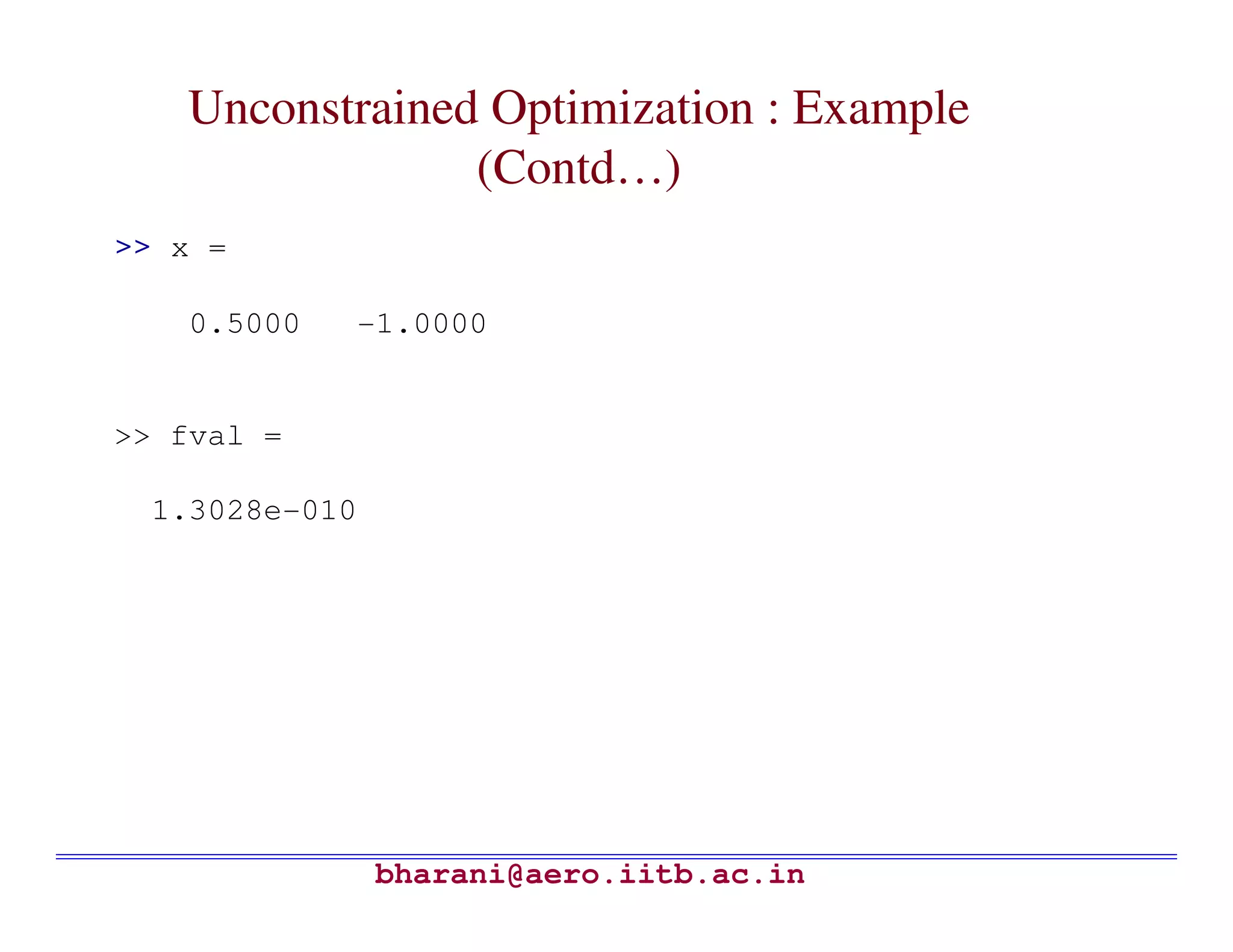
bharani@aero.iitb.ac.in Unonstrained Optimization :Example Consider the above problem with no constraints: Solution by MATLAB: Step 1: Create an inline object of the function to be minimized fun = inline('exp(x(1)) * (4*x(1)^2 + 2*x(2)^2 + 4*x(1)*x(2) + 2*x(2) + 1)'); Step 2: Take a guess at the solution: x0 = [-1 1]; Step 3: Solve using fminunc function: [x, fval] = fminunc(fun, x0); )12424()( 22 ++++= yxyyxexf x
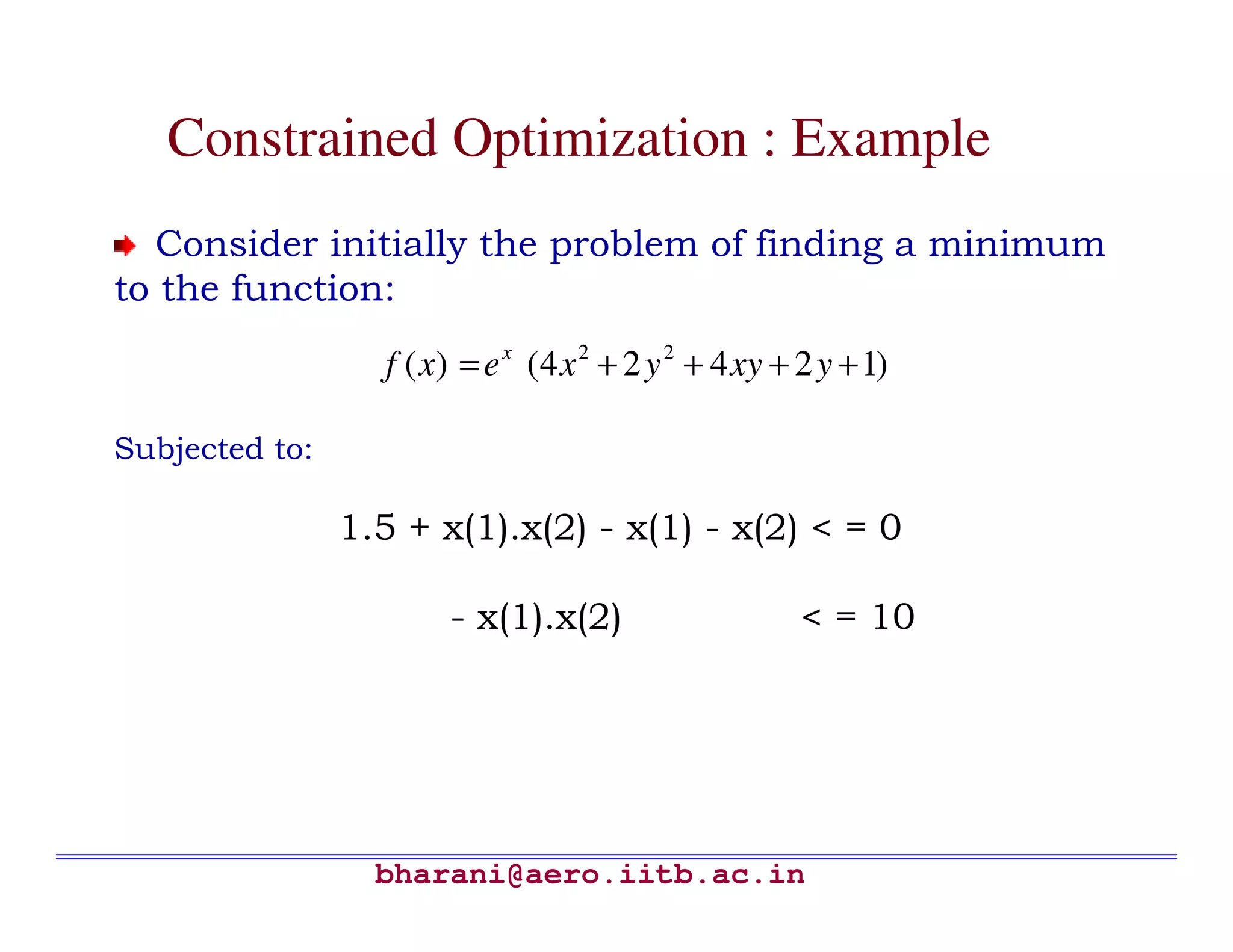
bharani@aero.iitb.ac.in Constrained Optimization :Example Consider initially the problem of finding a minimum to the function: Subjected to: 1.5 + x(1).x(2) - x(1) - x(2) < = 0 - x(1).x(2) < = 10 )12424()( 22 ++++= yxyyxexf x
54.
bharani@aero.iitb.ac.in Constrained Optimization :Example (contd…) Solution using MATLAB: Step 1: Write the m-file for objective function: function f = objfun(x) % objective function f=exp(x(1)) * (4*x(1)^2 + 2*x(2)^2 + 4*x(1)*x(2) + 2*x(2) + 1); Step 2: Write the m-file for constraints: function [c, ceq] = confun(x) % Nonlinear inequality constraints: c = [1.5 + x(1)*x(2) - x(1) - x(2); -x(1)*x(2) - 10]; % no nonlinear equality constraints: ceq = [];
55.
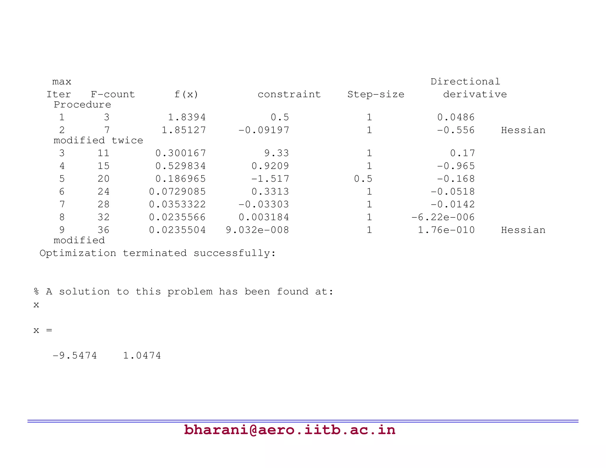
bharani@aero.iitb.ac.in Constrained Optimization :Example (contd…) Step 3: Take a guess at the solution x0 = [-1 1]; options = optimset('LargeScale','off','Display','iter'); % We have no linear equalities or inequalities or bounds, % so pass [] for those arguments [x,fval,exitflag,output] = fmincon('objfun',x0,[],[],[],[],[],[],'confun',options) ;
56.
bharani@aero.iitb.ac.in max Directional Iter F-countf(x) constraint Step-size derivative Procedure 1 3 1.8394 0.5 1 0.0486 2 7 1.85127 -0.09197 1 -0.556 Hessian modified twice 3 11 0.300167 9.33 1 0.17 4 15 0.529834 0.9209 1 -0.965 5 20 0.186965 -1.517 0.5 -0.168 6 24 0.0729085 0.3313 1 -0.0518 7 28 0.0353322 -0.03303 1 -0.0142 8 32 0.0235566 0.003184 1 -6.22e-006 9 36 0.0235504 9.032e-008 1 1.76e-010 Hessian modified Optimization terminated successfully: % A solution to this problem has been found at: x x = -9.5474 1.0474
57.
bharani@aero.iitb.ac.in % The functionvalue at the solution is: fval fval = 0.0236 % Both the constraints are active at the solution: [c, ceq] = confun(x) c = 1.0e-014 * 0.1110 -0.1776 ceq = []
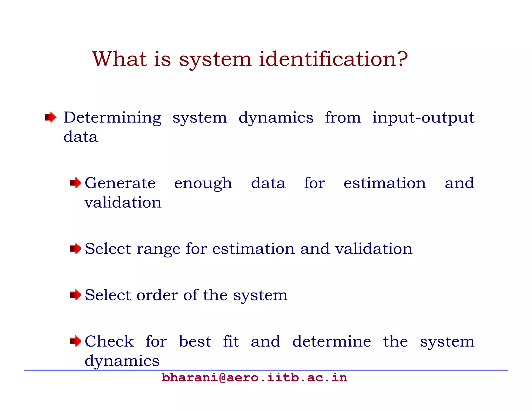
bharani@aero.iitb.ac.in What is systemidentification? Determining system dynamics from input-output data Generate enough data for estimation and validation Select range for estimation and validation Select order of the system Check for best fit and determine the system dynamics
63.
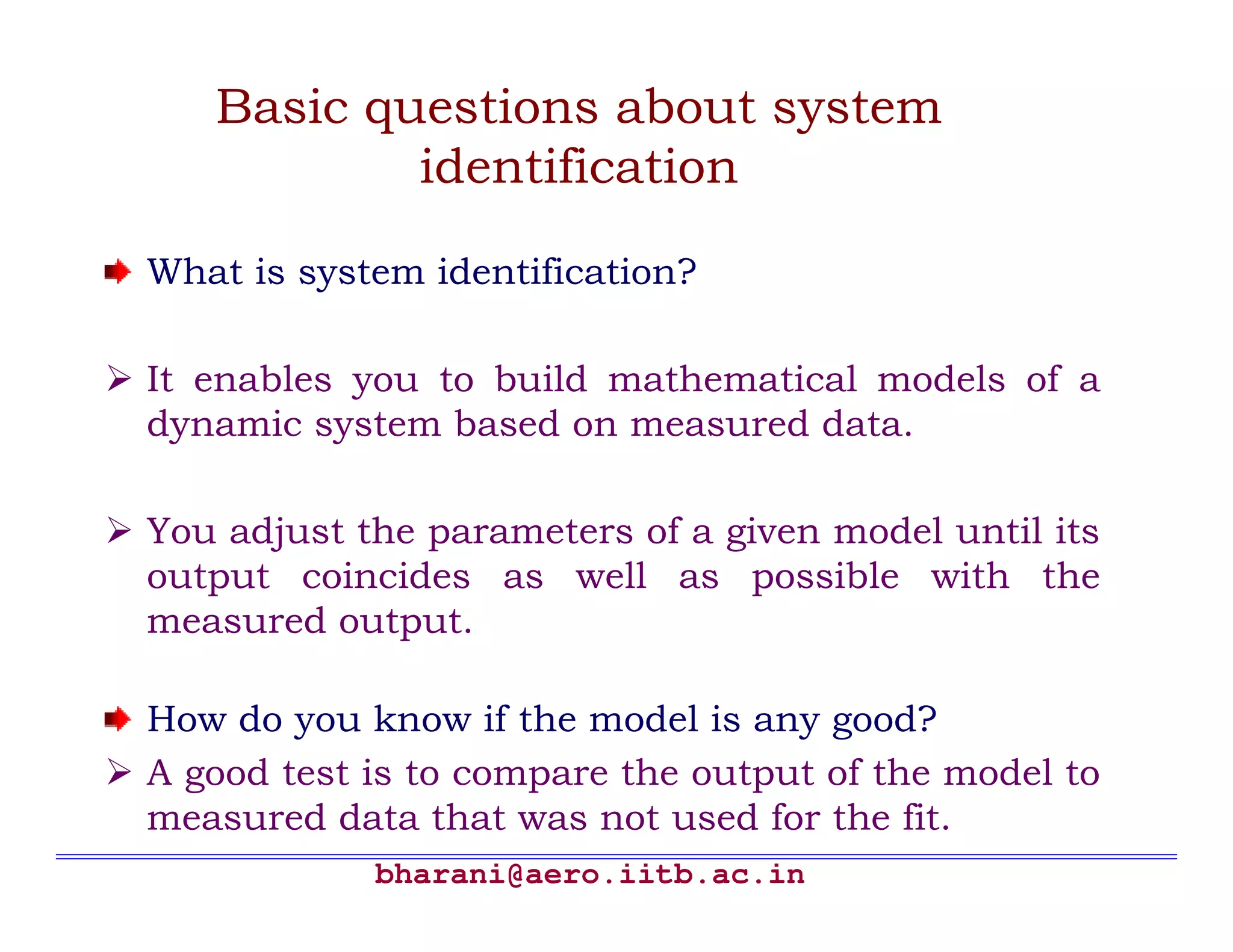
bharani@aero.iitb.ac.in Basic questions aboutsystem identification What is system identification? It enables you to build mathematical models of a dynamic system based on measured data. You adjust the parameters of a given model until its output coincides as well as possible with the measured output. How do you know if the model is any good? A good test is to compare the output of the model to measured data that was not used for the fit.
64.
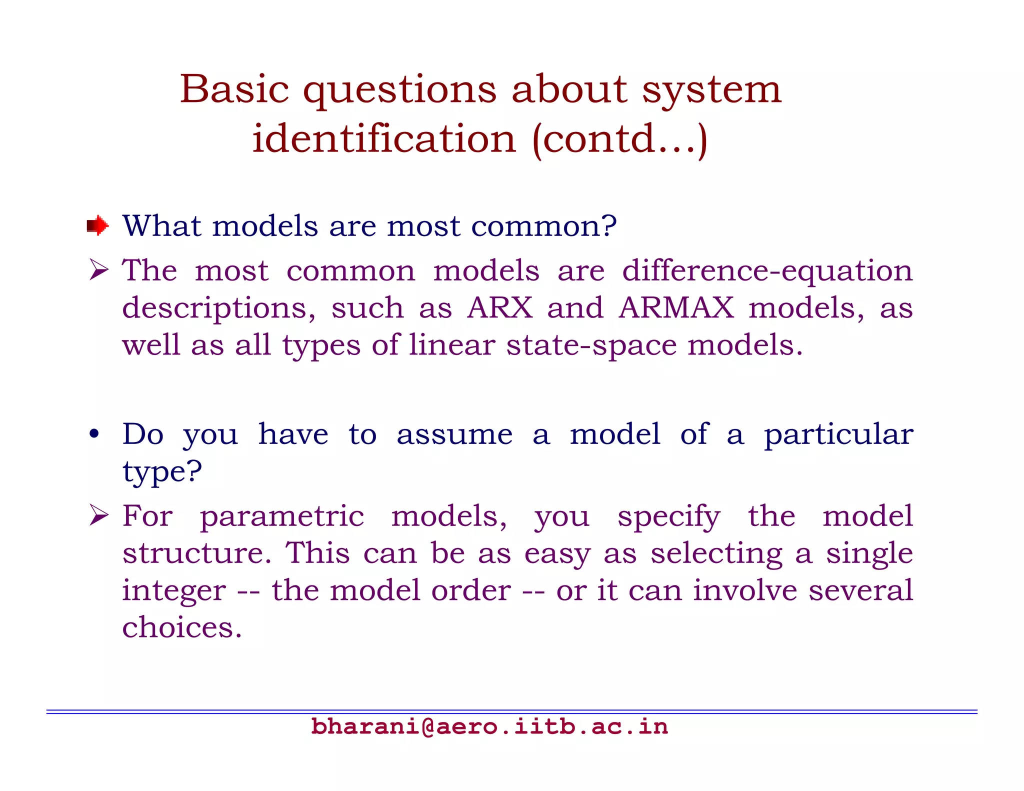
bharani@aero.iitb.ac.in Basic questions aboutsystem identification (contd…) What models are most common? The most common models are difference-equation descriptions, such as ARX and ARMAX models, as well as all types of linear state-space models. • Do you have to assume a model of a particular type? For parametric models, you specify the model structure. This can be as easy as selecting a single integer -- the model order -- or it can involve several choices.
65.
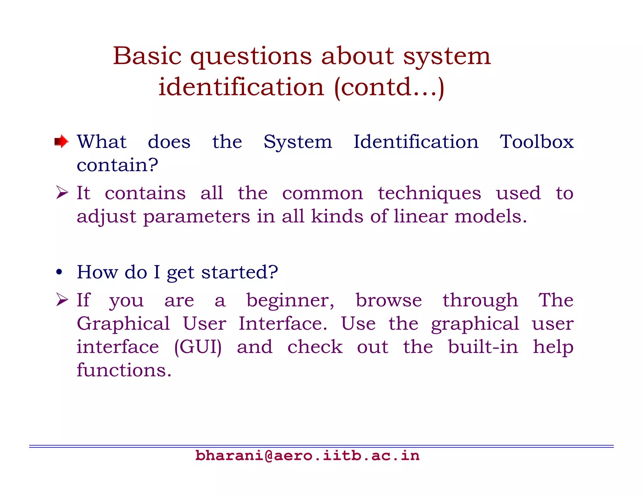
bharani@aero.iitb.ac.in Basic questions aboutsystem identification (contd…) What does the System Identification Toolbox contain? It contains all the common techniques used to adjust parameters in all kinds of linear models. • How do I get started? If you are a beginner, browse through The Graphical User Interface. Use the graphical user interface (GUI) and check out the built-in help functions.
66.
bharani@aero.iitb.ac.in Basic questions aboutsystem identification (contd…) Is this really all there is to system identification? There is a great deal written on the subject of system identification. However, the best way to explore system identification is by working with real data. It is important to remember that any estimated model, no matter how good it looks on your screen, is only a simplified reflection of reality.
67.
bharani@aero.iitb.ac.in Common terms usedin system identification Estimation data: The data set that is used to create a model of the data. Validation data: The data set (different from estimation data) that is used to validate the model. Model views: The various ways of inspecting the properties of a model, such as zeros and poles, as well as transient and frequency responses.
68.
bharani@aero.iitb.ac.in Common terms usedin system identification (contd…) Model sets or model structures are families of models with adjustable parameters. Parameter estimation is the process of finding the "best" values of these adjustable parameters. The system identification problem is to find both the model structure and good numerical values of the model parameters.
69.
bharani@aero.iitb.ac.in Common terms usedin system identification (contd…) • This is a matter of using numerical search to find those numerical values of the parameters that give the best agreement between the model's (simulated or predicted) output and the measured output. • Nonparametric identification methods: Techniques to estimate model behavior without necessarily using a given parameterized model set. • Model validation is the process of gaining confidence in a model.
bharani@aero.iitb.ac.in Basic Steps forSystem Identification Import data from the MATLAB workspace. Plot the data using Data Views. Preprocess the data using commands in the Preprocess menu. For example, you can remove constant offsets or linear trends (for linear models only), filter data, or select regions of interest.
72.
bharani@aero.iitb.ac.in Basic Steps forSystem Identification (contd…) Select estimation and validation data. Estimate models using commands in the Estimate menu. Validate models using Models Views. Export models to the MATLAB workspace for further processing .
bharani@aero.iitb.ac.in Introduction DSOLVE Symbolic solutionof ordinary differential equations. DSOLVE('eqn1','eqn2', ...) accepts symbolic equations representing ordinary differential equations and initial conditions. Several equations or initial conditions may be grouped together, separated by commas, in a single input argument. By default, the independent variable is 't'. The independent variable may be changed from 't' to some other symbolic variable by including that variable as the last input argument.
78.
bharani@aero.iitb.ac.in Introduction (contd…) The letter'D' denotes differentiation with respect to the independent variable, i.e. usually d/dt. A "D" followed by a digit denotes repeated differentiation; e.g., D2 is d^2/dt^2. Any characters immediately following these differentiation operators are taken to be the dependent variables; e.g., D3y denotes the third derivative of y(t). Note that the names of symbolic variables should not contain the letter "D".
79.
bharani@aero.iitb.ac.in Introduction (contd…) Initial conditionsare specified by equations like 'y(a)=b' or 'Dy(a) = b' where y is one of the dependent variables and a and b are constants. If the number of initial conditions given is less than the number of dependent variables, the resulting solutions will obtain arbitrary constants, C1, C2, etc. Three different types of output are possible. For one equation and one output, the resulting solution is returned, with multiple solutions to a nonlinear equation in a symbolic vector.
80.
bharani@aero.iitb.ac.in Introduction (contd…) If noclosed-form (explicit) solution is found, an implicit solution is attempted. When an implicit solution is returned, a warning is given. If neither an explicit nor implicit solution can be computed, then a warning is given and the empty sym is returned. In some cases concerning nonlinear equations, the output will be an equivalent lower order differential equation or an integral.
81.
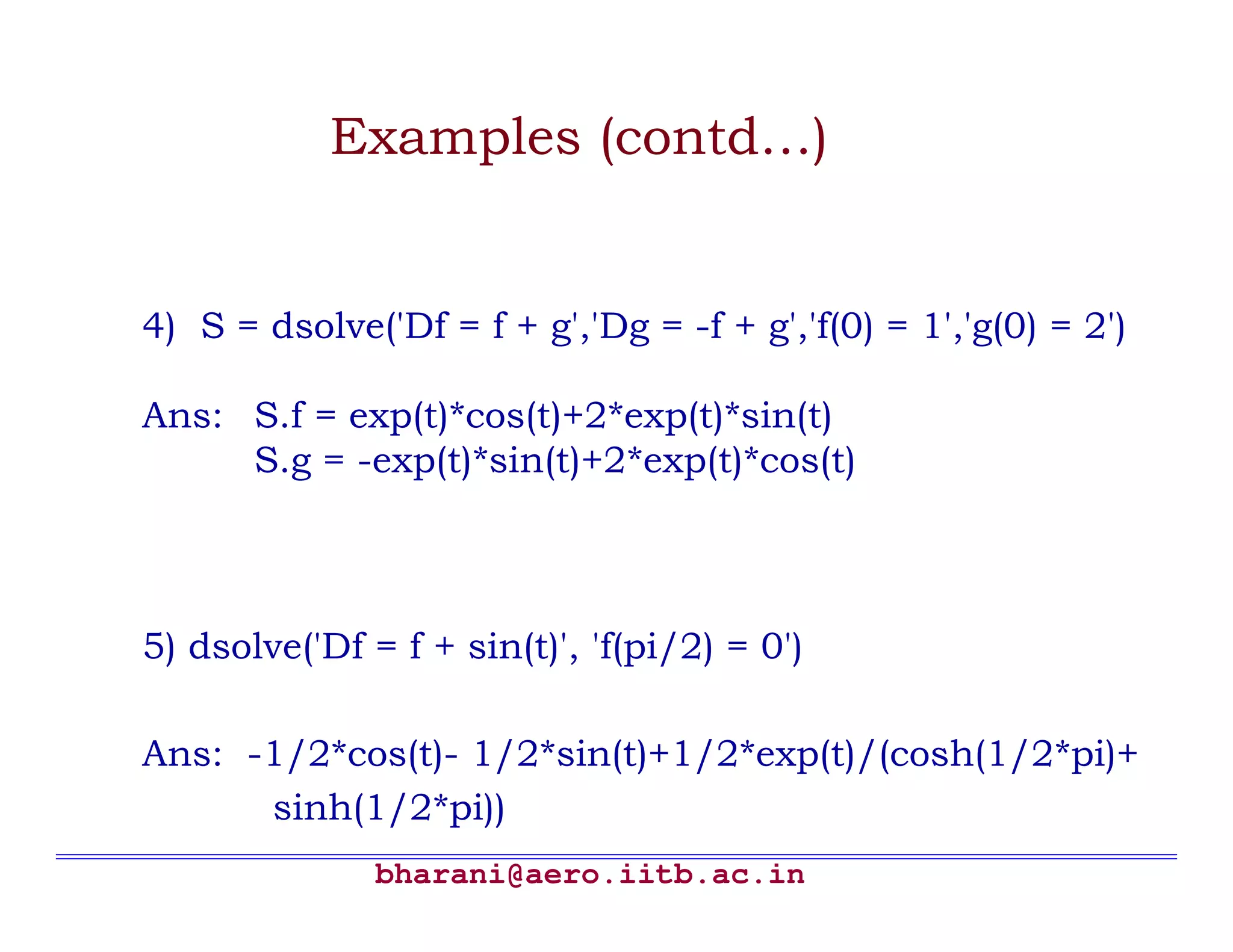
bharani@aero.iitb.ac.in Examples 1) dsolve('Dx =-a*x') returns ans: exp(-a*t)*C1 2) x = dsolve('Dx = -a*x','x(0) = 1','s') returns ans: x = exp(-a*s) 3) y = dsolve('(Dy)^2 + y^2 = 1','y(0) = 0') returns ans: y = [ sin(t)] [ -sin(t)]
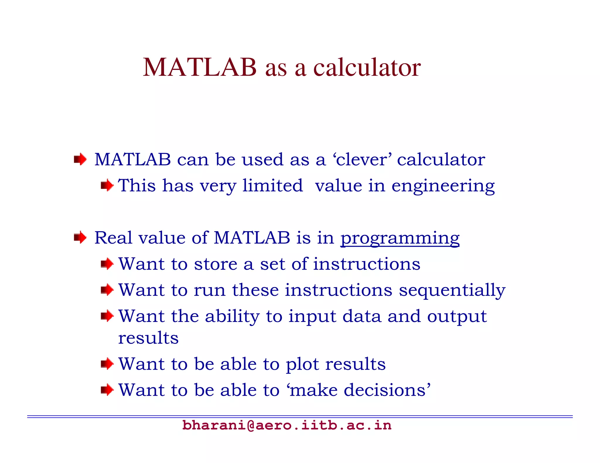
bharani@aero.iitb.ac.in MATLAB as acalculator MATLAB can be used as a ‘clever’ calculator This has very limited value in engineering Real value of MATLAB is in programming Want to store a set of instructions Want to run these instructions sequentially Want the ability to input data and output results Want to be able to plot results Want to be able to ‘make decisions’
86.
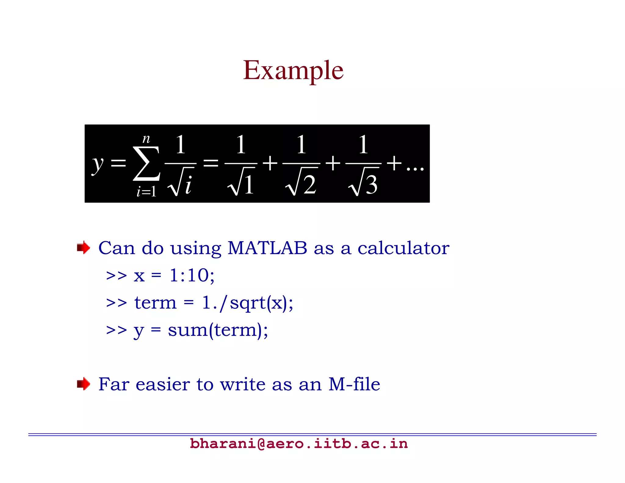
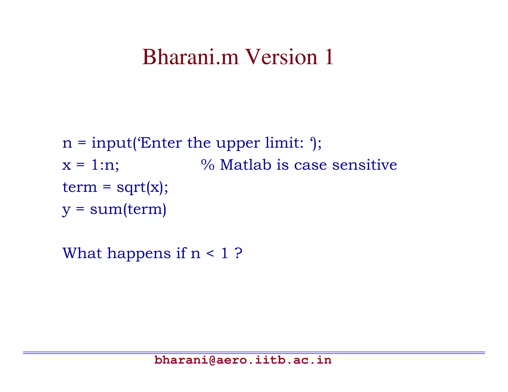
bharani@aero.iitb.ac.in Example Can do usingMATLAB as a calculator >> x = 1:10; >> term = 1./sqrt(x); >> y = sum(term); Far easier to write as an M-file ∑= +++== n i i y 1 ... 3 1 2 1 1 11
87.
bharani@aero.iitb.ac.in How to writean M-file File → New → M-file Takes you into the file editor Enter lines of code (nothing happens) Save file (we will call ours bharani.m) Run file Edit (ie modify) file if necessary
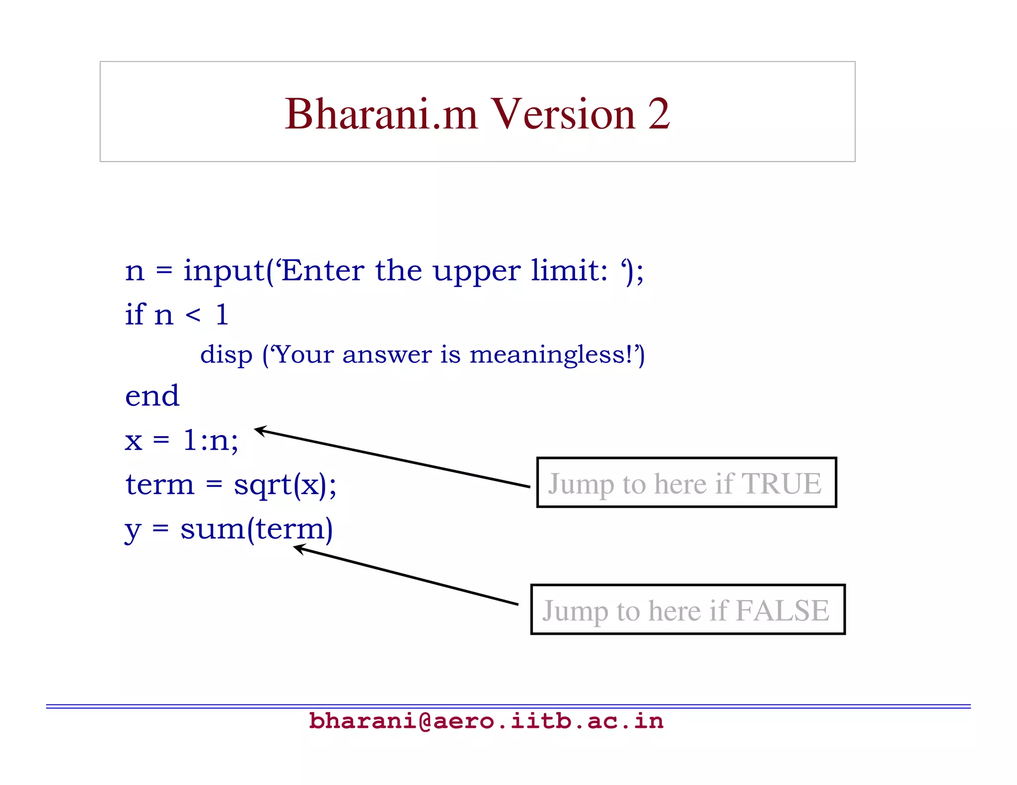
bharani@aero.iitb.ac.in Bharani.m Version 2 n= input(‘Enter the upper limit: ‘); if n < 1 disp (‘Your answer is meaningless!’) end x = 1:n; term = sqrt(x); y = sum(term) Jump to here if TRUE Jump to here if FALSE
90.
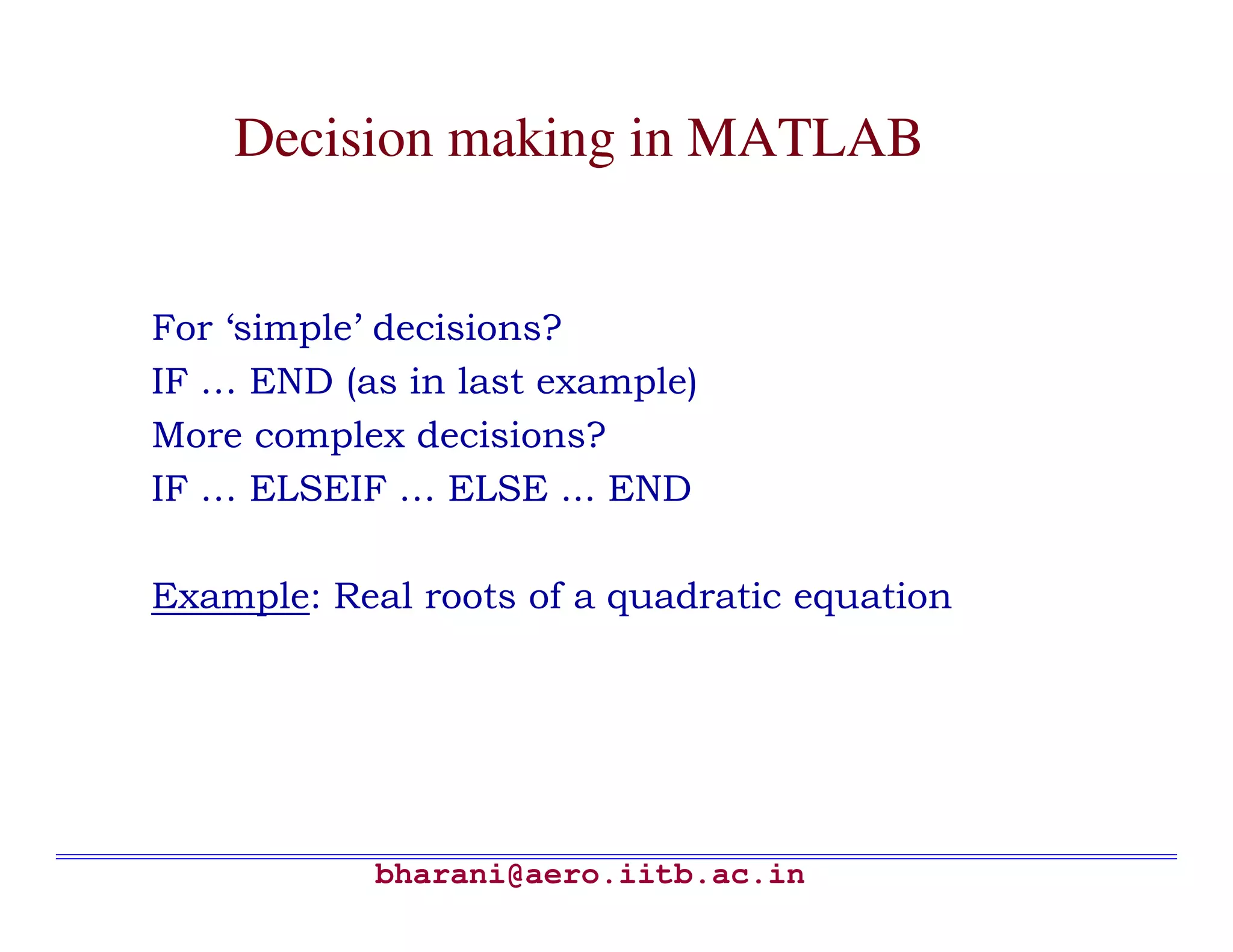
bharani@aero.iitb.ac.in Decision making inMATLAB For ‘simple’ decisions? IF … END (as in last example) More complex decisions? IF … ELSEIF … ELSE ... END Example: Real roots of a quadratic equation
91.
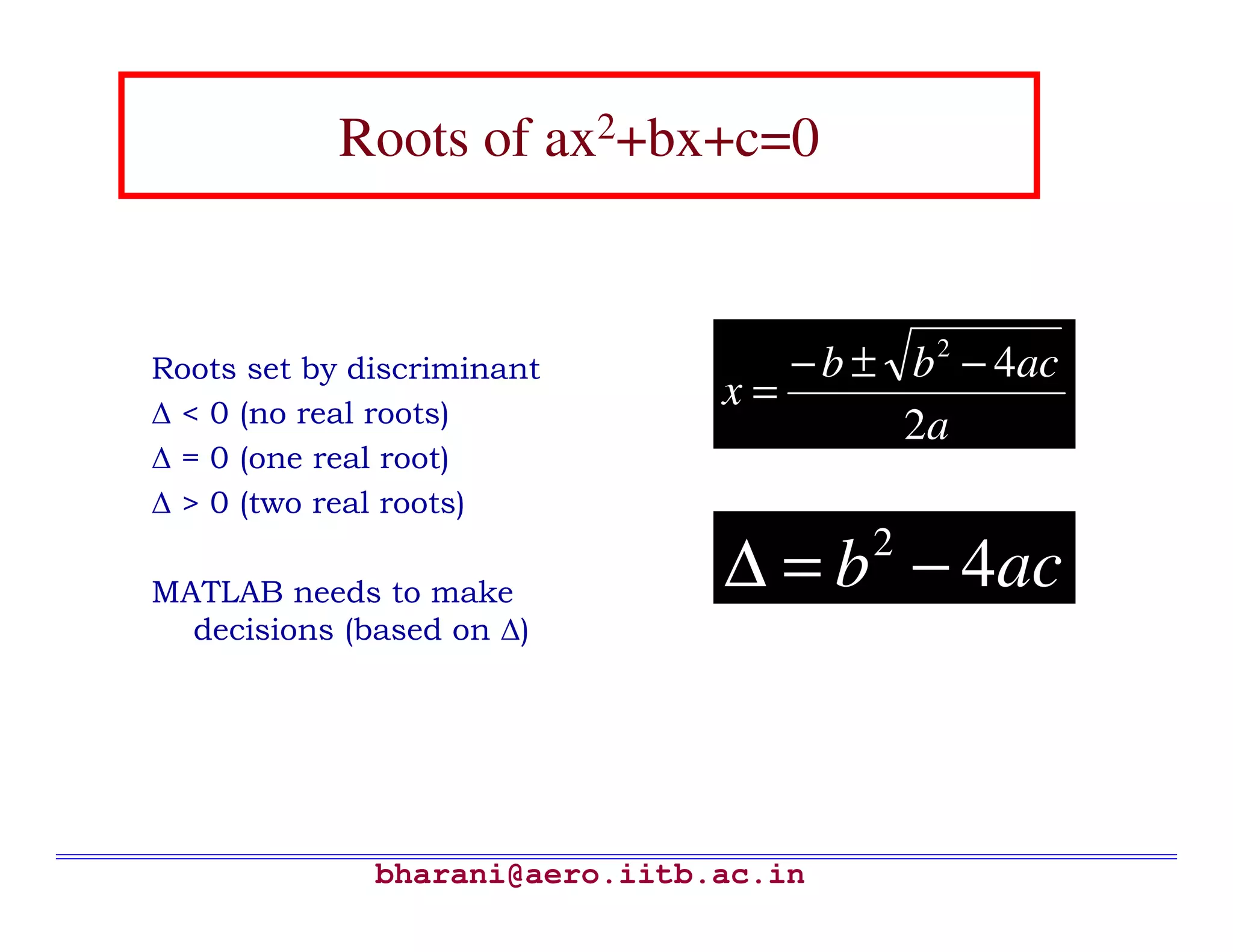
bharani@aero.iitb.ac.in Roots of ax2+bx+c=0 Rootsset by discriminant ∆ < 0 (no real roots) ∆ = 0 (one real root) ∆ > 0 (two real roots) MATLAB needs to make decisions (based on ∆) a acbb x 2 42 −±− = acb 42 −=∆
92.
bharani@aero.iitb.ac.in One possible M-file Readin values of a, b, c Calculate ∆ IF ∆ < 0 Print message ‘ No real roots’→ Go END ELSEIF ∆ = 0 Print message ‘One real root’→ Go END ELSE Print message ‘Two real roots’ END
93.
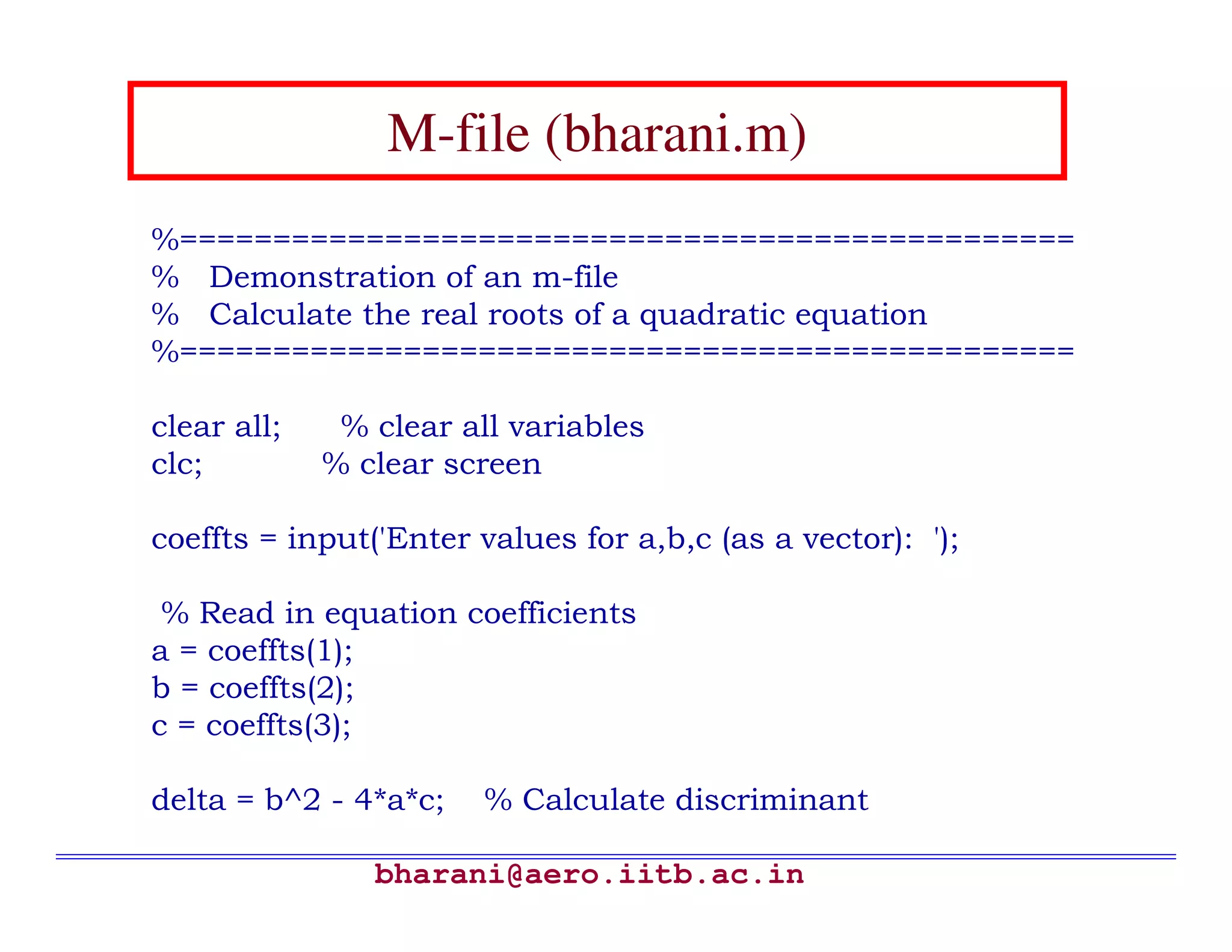
bharani@aero.iitb.ac.in M-file (bharani.m) %================================================ % Demonstrationof an m-file % Calculate the real roots of a quadratic equation %================================================ clear all; % clear all variables clc; % clear screen coeffts = input('Enter values for a,b,c (as a vector): '); % Read in equation coefficients a = coeffts(1); b = coeffts(2); c = coeffts(3); delta = b^2 - 4*a*c; % Calculate discriminant
94.
bharani@aero.iitb.ac.in M-file (bharani.m) (contd…) %Calculate number (and value) of real roots if delta < 0 fprintf('nEquation has no real roots:nn') disp(['discriminant = ', num2str(delta)]) elseif delta == 0 fprintf('nEquation has one real root:n') xone = -b/(2*a) else fprintf('nEquation has two real roots:n') x(1) = (-b + sqrt(delta))/(2*a); x(2) = (-b – sqrt(delta))/(2*a); fprintf('n First root = %10.2ent Second root = %10.2f', x(1),x(2)) end
95.
bharani@aero.iitb.ac.in Conclusions MATLAB is morethan a calculator its a powerful programming environment • Have reviewed: – Concept of an M-file – Decision making in MATLAB – IF … END and IF … ELSEIF … ELSE … END – Example of real roots for quadratic equation
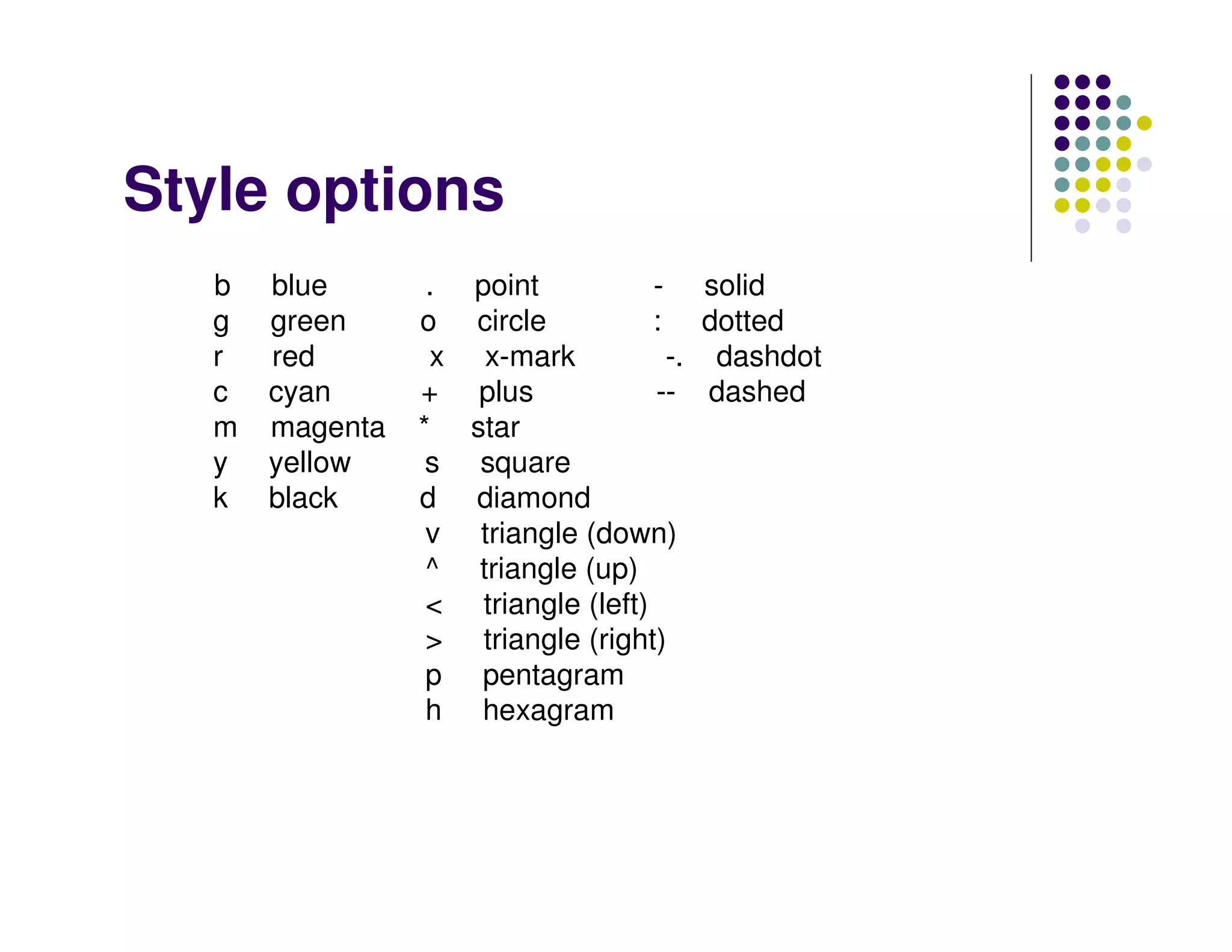
Style options b blue. point - solid g green o circle : dotted r red x x-mark -. dashdot c cyan + plus -- dashed m magenta * star y yellow s square k black d diamond v triangle (down) ^ triangle (up) < triangle (left) > triangle (right) p pentagram h hexagram
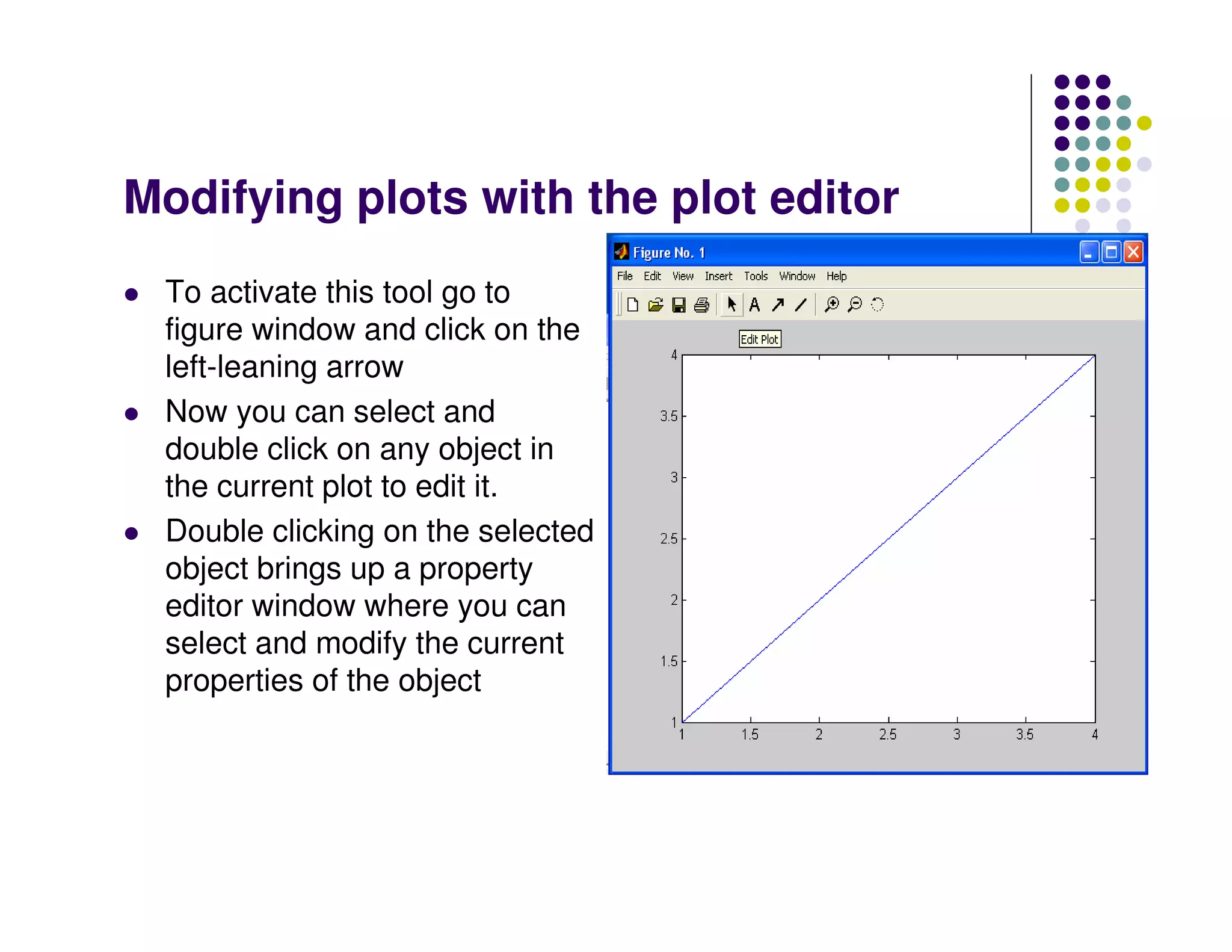
Modifying plots withthe plot editor To activate this tool go to figure window and click on the left-leaning arrow Now you can select and double click on any object in the current plot to edit it. Double clicking on the selected object brings up a property editor window where you can select and modify the current properties of the object
Handle Graphics Objects HandleGraphics is an object-oriented structure for creating, manipulating and displaying graphics Graphics in Matlab consist of objects Every graphics objects has: – a unique identifier, called handle – a set of characteristics, called properties
126.
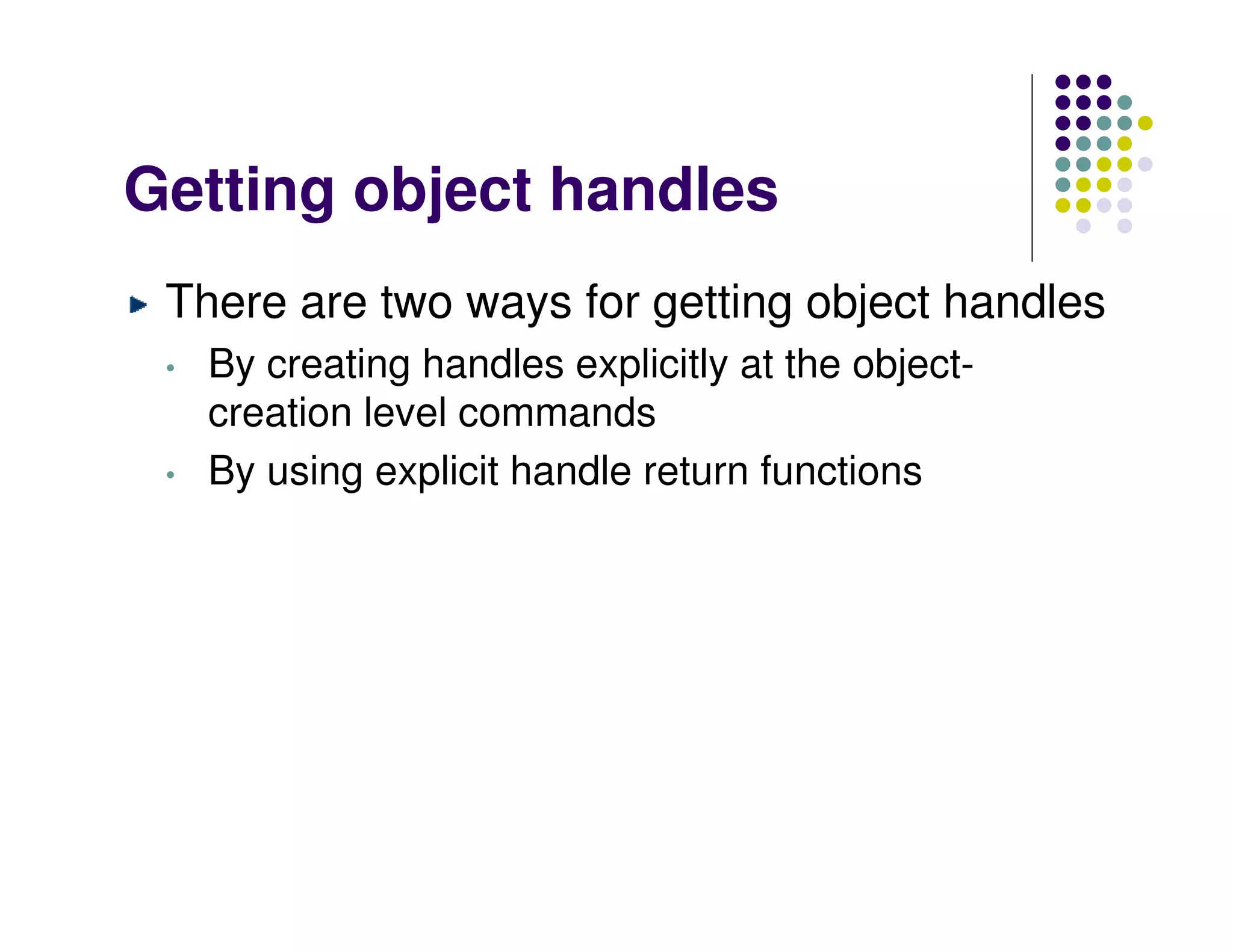
Getting object handles Thereare two ways for getting object handles • By creating handles explicitly at the object- creation level commands • By using explicit handle return functions
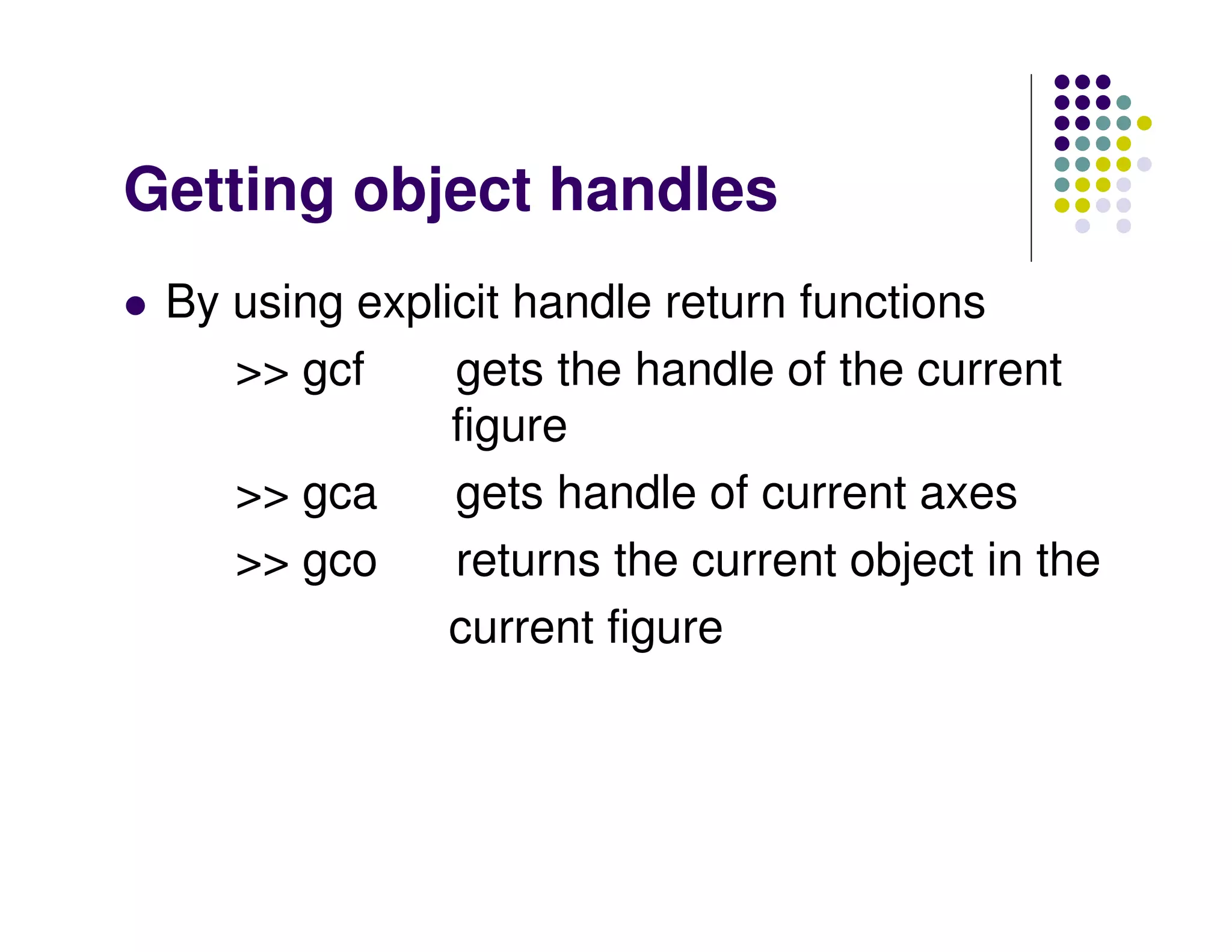
By using explicithandle return functions >> gcf gets the handle of the current figure >> gca gets handle of current axes >> gco returns the current object in the current figure Getting object handles
129.
Example >> figure >> axes >>line([1 2 3 4],[1 2 3 4]) >> hfig = gcf >> haxes = gca Click on the line in figure >>hL=gco Getting object handles
130.
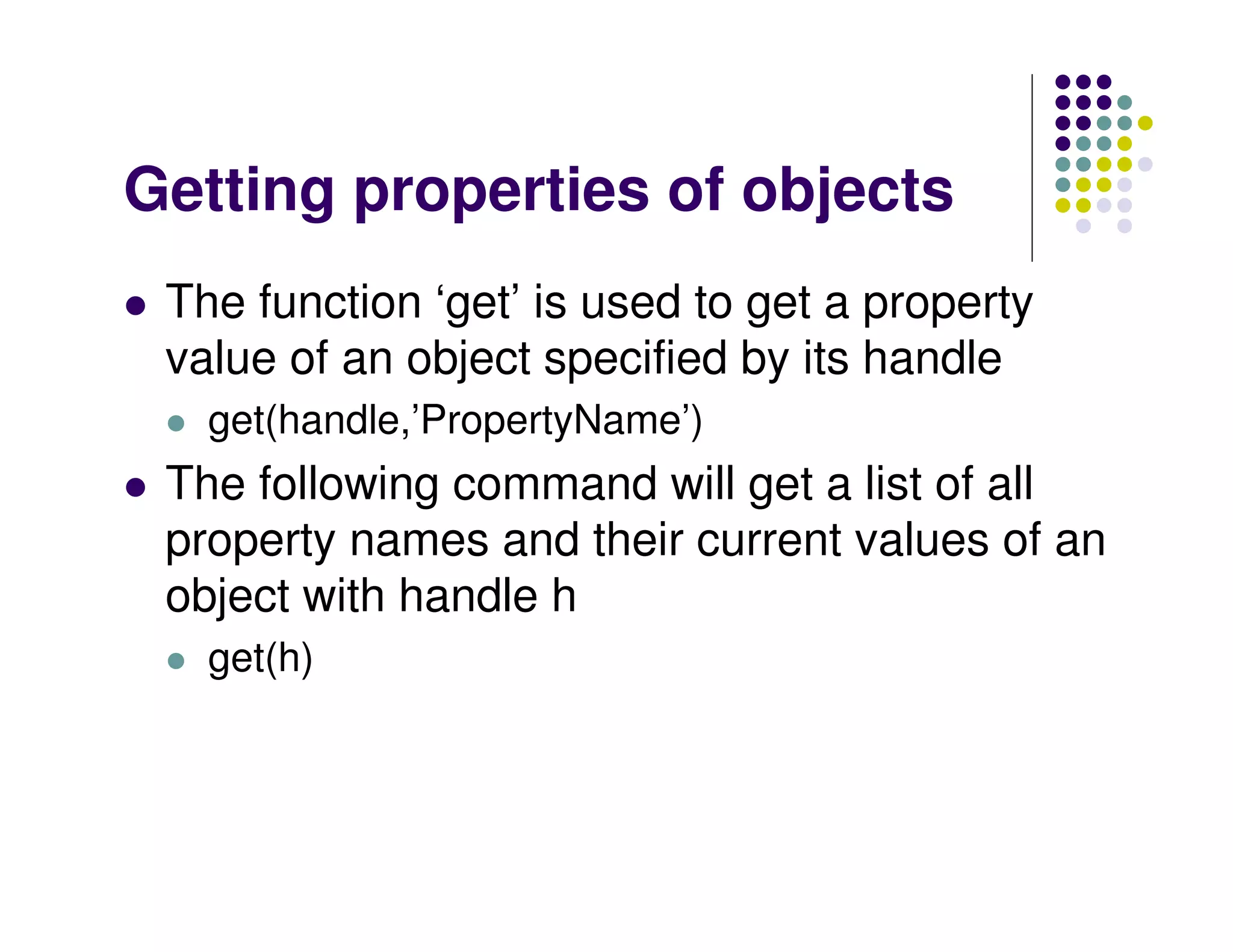
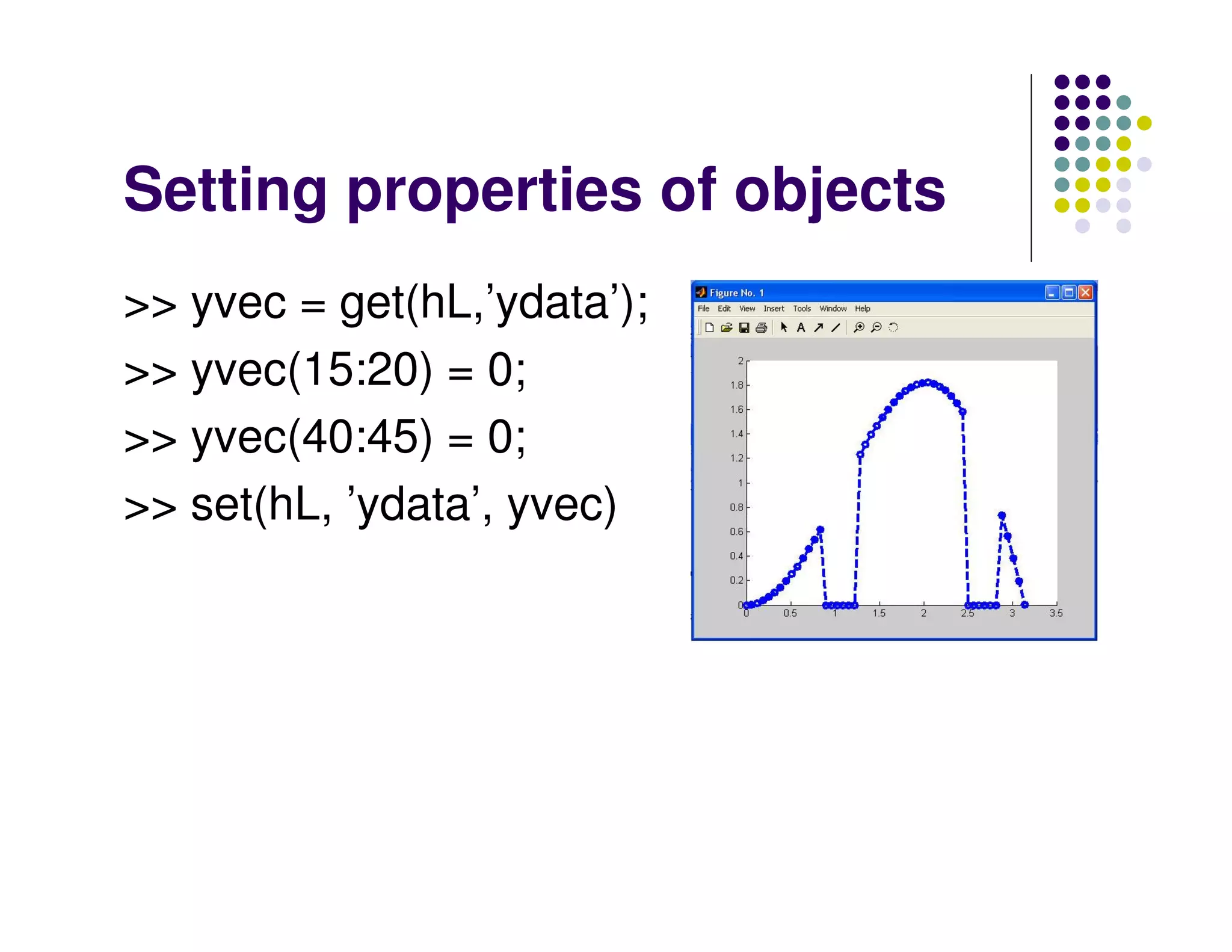
Getting properties ofobjects The function ‘get’ is used to get a property value of an object specified by its handle get(handle,’PropertyName’) The following command will get a list of all property names and their current values of an object with handle h get(h)
131.
Getting properties ofobjects Example >> h1=plot([ 1 2 3 4]);returns a line object >> get(h1) >> get(h1,’type’) >> get(h1,’linestyle’)
132.
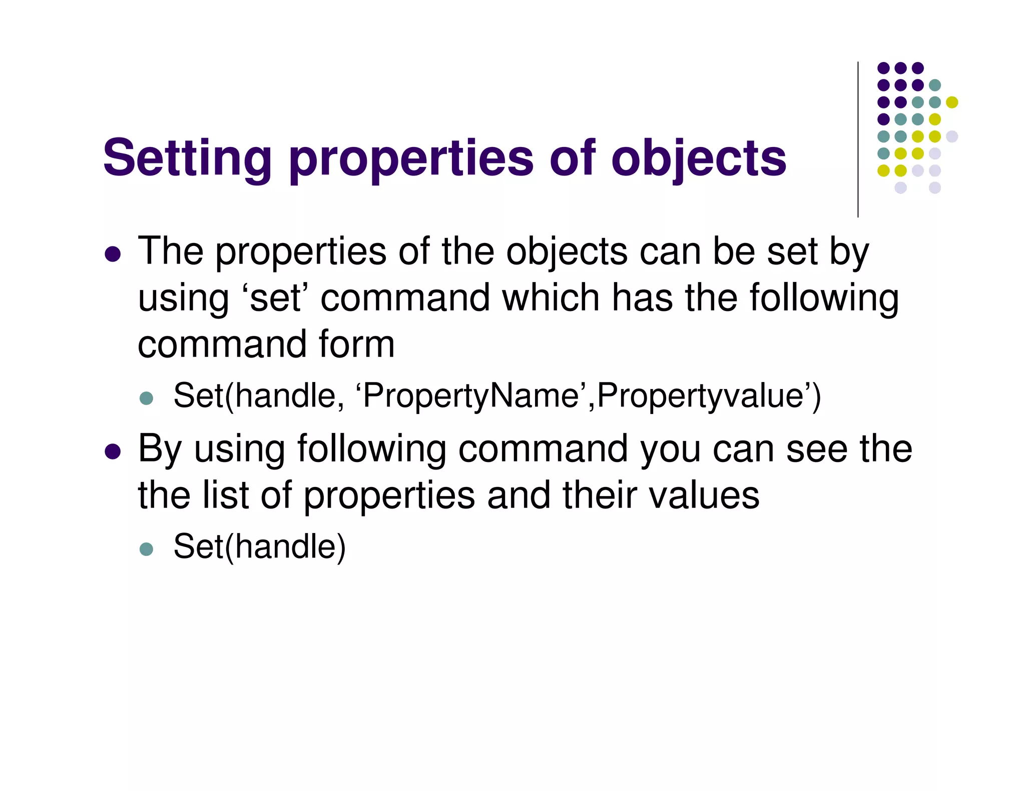
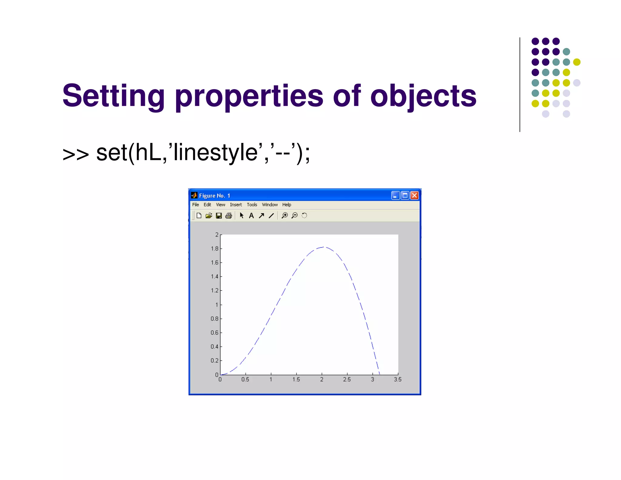
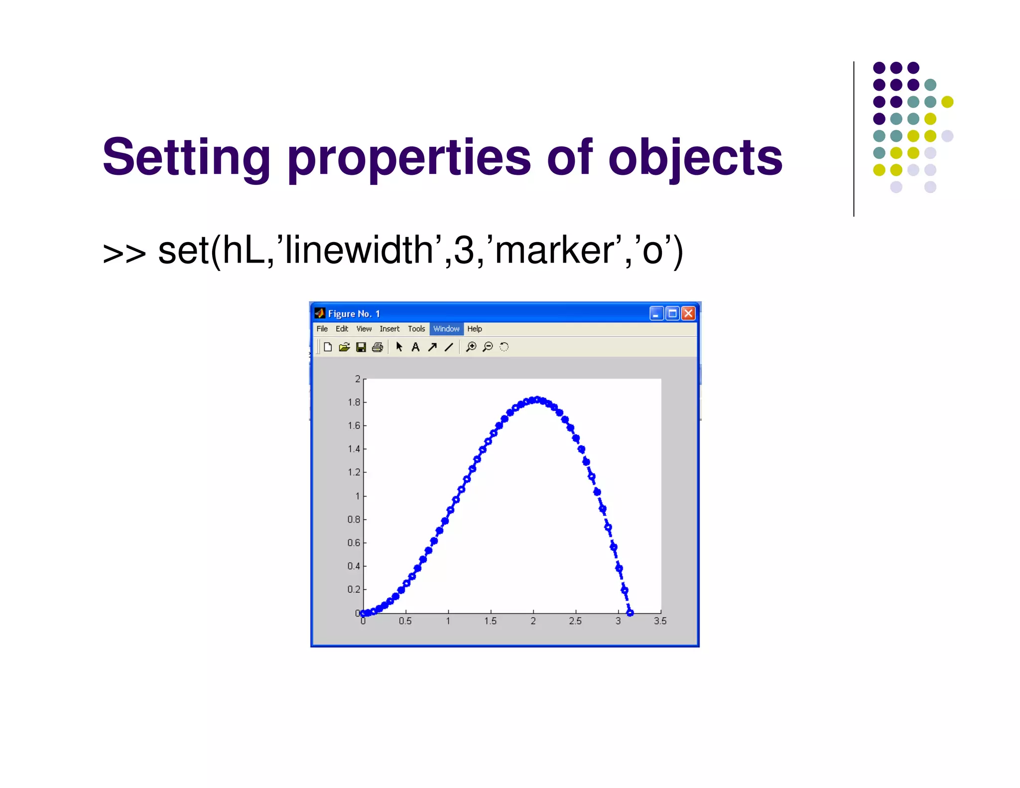
Setting properties ofobjects The properties of the objects can be set by using ‘set’ command which has the following command form Set(handle, ‘PropertyName’,Propertyvalue’) By using following command you can see the the list of properties and their values Set(handle)
133.
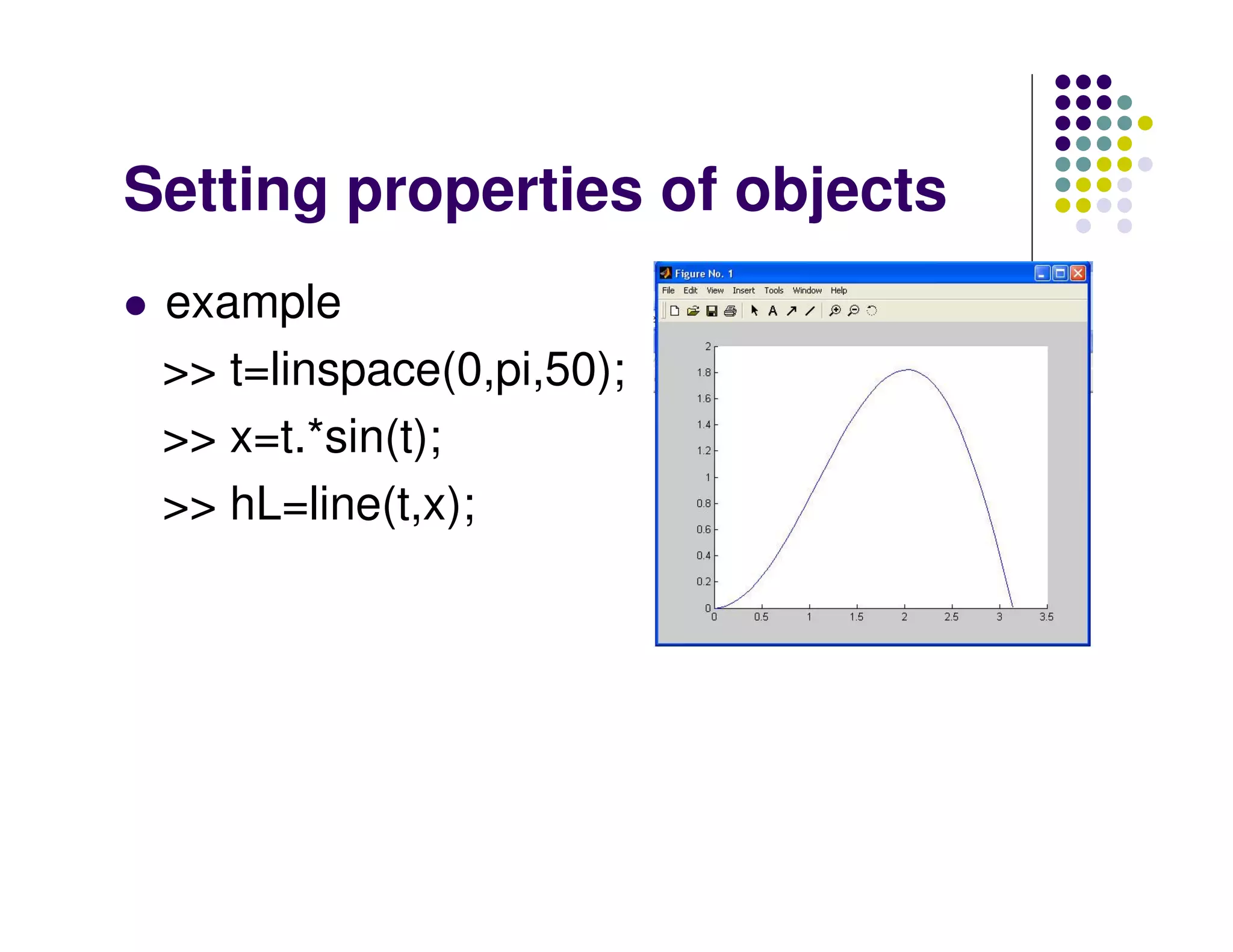
Setting properties ofobjects example >> t=linspace(0,pi,50); >> x=t.*sin(t); >> hL=line(t,x);


![bharani@aero.iitb.ac.in Matrices • A vector x = [1 2 5 1] x = 1 2 5 1 • A matrix x = [1 2 3; 5 1 4; 3 2 -1] x = 1 2 3 5 1 4 3 2 -1 • Transpose y = x.’ y = 1 2 5 1](https://image.slidesharecdn.com/matlabsolvedproblems-170720103318/75/Matlab-solved-problems-4-2048.jpg)
![bharani@aero.iitb.ac.in Matrices (Contd…) • x(i,j) subscription • whole row • whole column y = x(2,3) y = 4 y = x(3,:) y = 3 2 -1 y = x(:,2) y = 2 1 2 Let, x = [ 1 2 3 5 1 4 3 2 -1]](https://image.slidesharecdn.com/matlabsolvedproblems-170720103318/75/Matlab-solved-problems-5-2048.jpg)
![bharani@aero.iitb.ac.in Operators (in general) [ ] concatenation ( ) subscription x = [ zeros(1,3) ones(1,2) ] x = 0 0 0 1 1 x = [ 1 3 5 7 9] x = 1 3 5 7 9 y = x(2) y = 3 y = x(2:4) y = 3 5 7](https://image.slidesharecdn.com/matlabsolvedproblems-170720103318/75/Matlab-solved-problems-9-2048.jpg)
![bharani@aero.iitb.ac.in MATRIX OPERATIONS Let, A = eye(3) >> A = [ 1 0 0 0 1 0 0 0 1 ] >> eig(A) ans = 1 1 1 >> inv(A) ans = 1 0 0 0 1 0 0 0 1 >>A' ans = 1 0 0 0 1 0 0 0 1 >>A*A ans = 1 0 0 0 1 0 0 0 1](https://image.slidesharecdn.com/matlabsolvedproblems-170720103318/75/Matlab-solved-problems-10-2048.jpg)
![bharani@aero.iitb.ac.in MATRIX OPERATIONS (Contd…) Let, >> A = [1 2 3;4 5 6;7 8 9] A = [ 1 2 3 4 5 6 7 8 9 ] >> eig(A) ans = 16.1168 -1.1168 -0.0000 >> B=A' B = 1 4 7 2 5 8 3 6 9 >>C=A*B C = 14 32 50 32 77 122 50 122 194 >> D=A.*B D = 1 8 21 8 25 48 21 48 81](https://image.slidesharecdn.com/matlabsolvedproblems-170720103318/75/Matlab-solved-problems-11-2048.jpg)

![bharani@aero.iitb.ac.in Linear Algebra Solving a linear system Find the values of x, y and z for the following equations: 5x = 3y – 2z +10 8y +4z = 3x + 20 2x + 4y - 9z = 9 Step 1: Rearrange equations: 5x - 3y + 2z = 10 - 3x + 8y +4z = 20 2x + 4y - 9z = 9 Step 2: Write the equations in matrix form: [A] x = b − − − = 942 483 235 A = 9 20 10 b](https://image.slidesharecdn.com/matlabsolvedproblems-170720103318/75/Matlab-solved-problems-15-2048.jpg)
![bharani@aero.iitb.ac.in Linear Algebra (Contd…) Step 3: Solve the matrix equation in MATLAB: >> A = [ 5 -3 2; -3 8 4; 2 4 -9]; >> b = [10; 20; 9] >> x = A b x = 3.442 3.1982 1.1868 % Veification >> c = A*x >> c = 10.0000 20.0000 9.0000](https://image.slidesharecdn.com/matlabsolvedproblems-170720103318/75/Matlab-solved-problems-16-2048.jpg)
![bharani@aero.iitb.ac.in Method 2: By using MATLAB: Step 1: Enter matrix A and type [V, D] = eig(A) >> A = [ 5 -3 2; -3 8 4; 2 4 -9]; >> [V, D] = eig(A) V = -0.1709 0.8729 0.4570 -0.2365 0.4139 -0.8791 0.9565 0.2583 -0.1357 D = -10.3463 0 0 0 4.1693 0 0 0 10.1770 Linear Algebra (Contd…)](https://image.slidesharecdn.com/matlabsolvedproblems-170720103318/75/Matlab-solved-problems-18-2048.jpg)
![bharani@aero.iitb.ac.in Curve Fitting (Contd…) Example 1 : straight line (linear) fit: Step 1: Plot raw data: Enter the data in MATLAB and plot it: >> x = [ 5 10 20 50 100]; >> y = [15 33 53 140 301]; >> plot (x,y,’o’) >> grid 301140533315Y 1005020105x](https://image.slidesharecdn.com/matlabsolvedproblems-170720103318/75/Matlab-solved-problems-22-2048.jpg)
![bharani@aero.iitb.ac.in Interpolation (Contd…) Example: x = [1 2 3 4 5 6 7 8 9] y = [1 4 9 16 25 36 49 64 81] Find the value of 5.5? Method 1: Linear Interpolation MATLAB Command : >> yi=interp1(x,y,5.5,'linear') yi = 30.5000](https://image.slidesharecdn.com/matlabsolvedproblems-170720103318/75/Matlab-solved-problems-29-2048.jpg)
![bharani@aero.iitb.ac.in Data Analysis and statistics (Contd…) Example: x = [1 2 3 4 5 6 7 8 9] y = [1 4 9 16 25 36 49 64 81] Find the minimum value, maximum value, mean, median?](https://image.slidesharecdn.com/matlabsolvedproblems-170720103318/75/Matlab-solved-problems-32-2048.jpg)
![bharani@aero.iitb.ac.in Data Analysis and statistics (Contd…) It can be performed directly by using MATLAB commands also: Consider: x = [1 2 3 4 5] mean (x) : Gives arithmetic mean of ‘x’ or the avg. data. MATLAB usage: mean (x) gives 3. median (x) : gives the middle value or arithmetic mean of two middle Numbers. MATLAB usage: median (x) gives 3. Std(x): gives the standard deviation Max(x)/min(x): gives the largest/smallest value](https://image.slidesharecdn.com/matlabsolvedproblems-170720103318/75/Matlab-solved-problems-36-2048.jpg)


![bharani@aero.iitb.ac.in X = FMINCON(FUN,X0,A,B) starts at X0 and finds a minimum X to the function FUN, subject to the linear inequalities A*X <= B. X=FMINCON(FUN,X0,A,B,Aeq,Beq) minimizes FUN subject to the linear equalities: Aeq*X = Beq as well as A*X <= B. (Set A=[ ] and B=[ ] if no inequalities exist.) Optimization through MATLAB (Contd…)](https://image.slidesharecdn.com/matlabsolvedproblems-170720103318/75/Matlab-solved-problems-49-2048.jpg)
![bharani@aero.iitb.ac.in Unonstrained Optimization : Example Consider the above problem with no constraints: Solution by MATLAB: Step 1: Create an inline object of the function to be minimized fun = inline('exp(x(1)) * (4*x(1)^2 + 2*x(2)^2 + 4*x(1)*x(2) + 2*x(2) + 1)'); Step 2: Take a guess at the solution: x0 = [-1 1]; Step 3: Solve using fminunc function: [x, fval] = fminunc(fun, x0); )12424()( 22 ++++= yxyyxexf x](https://image.slidesharecdn.com/matlabsolvedproblems-170720103318/75/Matlab-solved-problems-51-2048.jpg)
![bharani@aero.iitb.ac.in Constrained Optimization : Example (contd…) Solution using MATLAB: Step 1: Write the m-file for objective function: function f = objfun(x) % objective function f=exp(x(1)) * (4*x(1)^2 + 2*x(2)^2 + 4*x(1)*x(2) + 2*x(2) + 1); Step 2: Write the m-file for constraints: function [c, ceq] = confun(x) % Nonlinear inequality constraints: c = [1.5 + x(1)*x(2) - x(1) - x(2); -x(1)*x(2) - 10]; % no nonlinear equality constraints: ceq = [];](https://image.slidesharecdn.com/matlabsolvedproblems-170720103318/75/Matlab-solved-problems-54-2048.jpg)
![bharani@aero.iitb.ac.in Constrained Optimization : Example (contd…) Step 3: Take a guess at the solution x0 = [-1 1]; options = optimset('LargeScale','off','Display','iter'); % We have no linear equalities or inequalities or bounds, % so pass [] for those arguments [x,fval,exitflag,output] = fmincon('objfun',x0,[],[],[],[],[],[],'confun',options) ;](https://image.slidesharecdn.com/matlabsolvedproblems-170720103318/75/Matlab-solved-problems-55-2048.jpg)
![bharani@aero.iitb.ac.in % The function value at the solution is: fval fval = 0.0236 % Both the constraints are active at the solution: [c, ceq] = confun(x) c = 1.0e-014 * 0.1110 -0.1776 ceq = []](https://image.slidesharecdn.com/matlabsolvedproblems-170720103318/75/Matlab-solved-problems-57-2048.jpg)


![bharani@aero.iitb.ac.in Examples 1) dsolve('Dx = -a*x') returns ans: exp(-a*t)*C1 2) x = dsolve('Dx = -a*x','x(0) = 1','s') returns ans: x = exp(-a*s) 3) y = dsolve('(Dy)^2 + y^2 = 1','y(0) = 0') returns ans: y = [ sin(t)] [ -sin(t)]](https://image.slidesharecdn.com/matlabsolvedproblems-170720103318/75/Matlab-solved-problems-81-2048.jpg)


![bharani@aero.iitb.ac.in M-file (bharani.m) (contd…) % Calculate number (and value) of real roots if delta < 0 fprintf('nEquation has no real roots:nn') disp(['discriminant = ', num2str(delta)]) elseif delta == 0 fprintf('nEquation has one real root:n') xone = -b/(2*a) else fprintf('nEquation has two real roots:n') x(1) = (-b + sqrt(delta))/(2*a); x(2) = (-b – sqrt(delta))/(2*a); fprintf('n First root = %10.2ent Second root = %10.2f', x(1),x(2)) end](https://image.slidesharecdn.com/matlabsolvedproblems-170720103318/75/Matlab-solved-problems-94-2048.jpg)


![Simple plot >> a=[1 2 3 4] >> plot(a)](https://image.slidesharecdn.com/matlabsolvedproblems-170720103318/75/Matlab-solved-problems-100-2048.jpg)

![Labels, title, legend and other text objects >> a=[1 2 3 4]; b=[ 1 2 3 4]; c=[4 5 6 7] >> plot(a,b,a,c) >> grid >> xlabel(‘xaxis’) >> ylabel(‘yaxis’) >> title(‘example’) >> legend(‘first’,’second’) >> text(2,6,’plot’)](https://image.slidesharecdn.com/matlabsolvedproblems-170720103318/75/Matlab-solved-problems-108-2048.jpg)
![Zoom in and zoom out >> figure >> plot(t,sin(t)) >> axis([0 2 -2 2])](https://image.slidesharecdn.com/matlabsolvedproblems-170720103318/75/Matlab-solved-problems-113-2048.jpg)
![Specialised plotting routines >> stem(t,sin(t)); >> bar(t,sin(t)) >> a=[1 2 3 4]; stairs(a);](https://image.slidesharecdn.com/matlabsolvedproblems-170720103318/75/Matlab-solved-problems-115-2048.jpg)

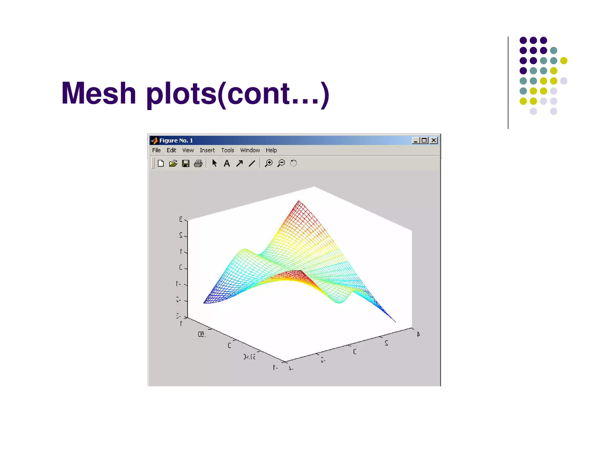
![Mesh plots >> x=linspace(-3,3,50); >> [X,Y]= meshgrid(x,y); >> Z=X.*Y.*(X.^2-Y.^2)./(X.^2+Y.^2); >> mesh(X,Y,Z); >> figure(2)](https://image.slidesharecdn.com/matlabsolvedproblems-170720103318/75/Matlab-solved-problems-120-2048.jpg)
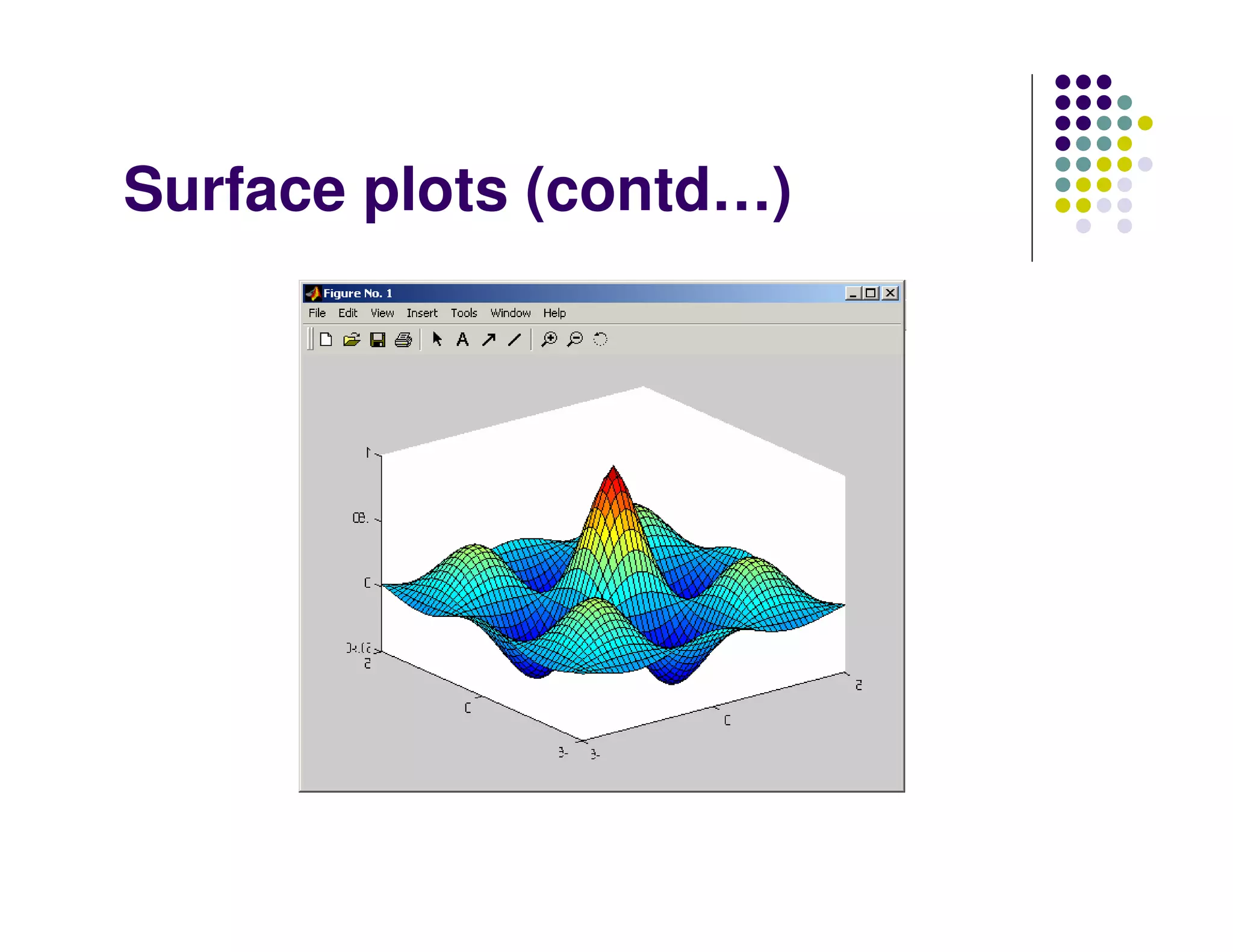
![Surface plots >> u = -5 : 0.2 : 5; >> [X,Y] = meshgrid(u,u); >> Z=cos(X).*cos(Y).*exp(-sqrt(X.^2+Y.^2)/4); >> surf(X,Y,Z)](https://image.slidesharecdn.com/matlabsolvedproblems-170720103318/75/Matlab-solved-problems-122-2048.jpg)


![Getting object handles By creating handles explicitly at the object- creation level commands >> hfig=figure >> haxes=axes(‘position’,[0.1 0.1 0.4 0.4]) >> t=linspace(0,pi,10); >> hL = line(t,sin(t)) >> hx1 = xlabel(‘Angle’)](https://image.slidesharecdn.com/matlabsolvedproblems-170720103318/75/Matlab-solved-problems-127-2048.jpg)
![Example >> figure >> axes >> line([1 2 3 4],[1 2 3 4]) >> hfig = gcf >> haxes = gca Click on the line in figure >>hL=gco Getting object handles](https://image.slidesharecdn.com/matlabsolvedproblems-170720103318/75/Matlab-solved-problems-129-2048.jpg)
![Getting properties of objects Example >> h1=plot([ 1 2 3 4]);returns a line object >> get(h1) >> get(h1,’type’) >> get(h1,’linestyle’)](https://image.slidesharecdn.com/matlabsolvedproblems-170720103318/75/Matlab-solved-problems-131-2048.jpg)
![Creating subplots using axes command >> hfig=figure >> ha1=axes(‘position’,[0.1 0.5 0.3 0.3]) >> line([1 2 3 4],[1 2 3 4]) >> ha2=axes(‘position’[0.5 0.5 0.3 0.3]) >> line([1 2 3 4],[ 1 10 100 1000]) >> ha3=axes(‘position’,[0.1 0.1 0.3 0.3]) >> line([1 2 3 4],[0.1 0.2 0.3 0.4]) >> ha4=axes(‘position’,[0.5 0.1 0.3 0.3]) >> line([1 2 3 4],[10 10 10 10])](https://image.slidesharecdn.com/matlabsolvedproblems-170720103318/75/Matlab-solved-problems-137-2048.jpg)