Introduction to MATLAB Programming for Engineers

INTRODUCTORY LECTURE ON MATLAB

Topics • Introduction • MATLAB Environment • Getting Help • Variables • Vectors, Matrices and Linear Algebra • Plotting

Introduction What is MATALB?  MATLAB is a computer program that combines computation and visualization power that makes it particularly useful tool for engineers.  MATLAB is an executive program, and a script can be made with a list of MATLAB commands like other programming language. MATLAB stands for MATrix LABoratory.  The system was designed to make matrix computation particularly easy. The MATLAB environment allows the user to:  manage variables  import and export data  perform calculation  generate plots  develop and manage files for use with MATLAB.

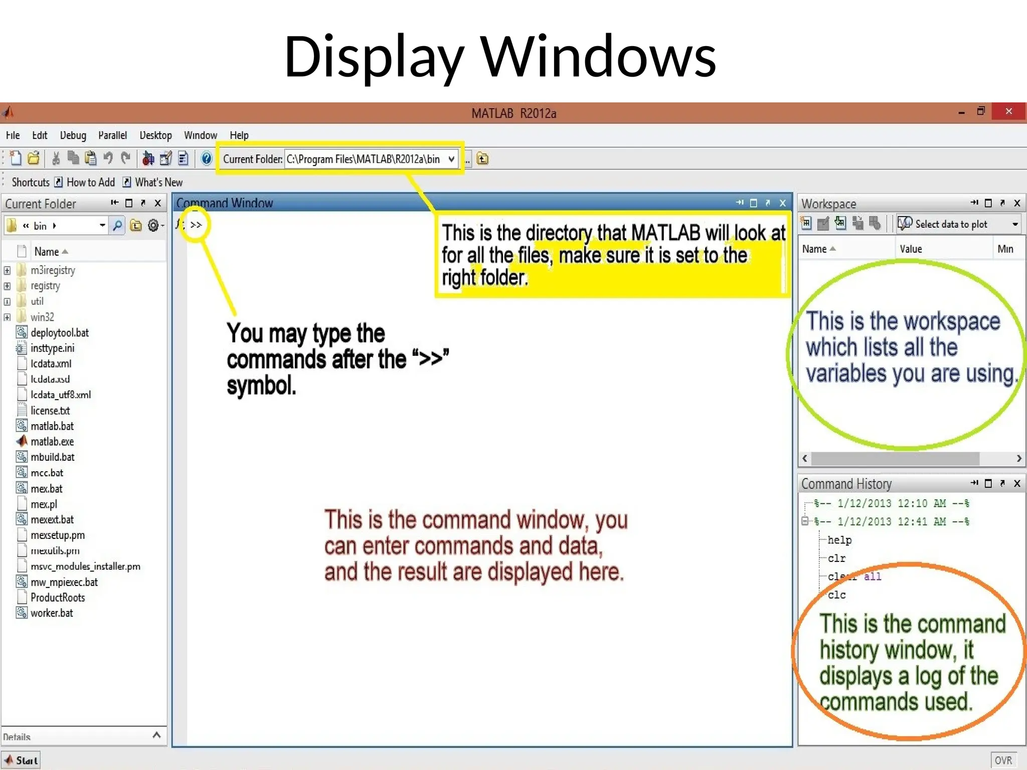
MATLAB Environment To start MATLAB: START → PROGRAMS → MATLAB 2012a → MATLAB 2012a OR shortcut creation/activation on the desktop

Display Windows (con't...) • Graphic (Figure) window –Displays plots and graphs –Created in response to graphics commands. • M-file editor/debugger window –Create and edit scripts of commands called M- files.

Getting Help • Type one of following commands in the command window: – help - lists all the help topic – help topic - provides help for the specified topic – help command - provides help for the specified command • help help - provides information on use of the help command – helpwin - opens a separate help window for navigation – lookfor keyword - Search all M-files for keyword

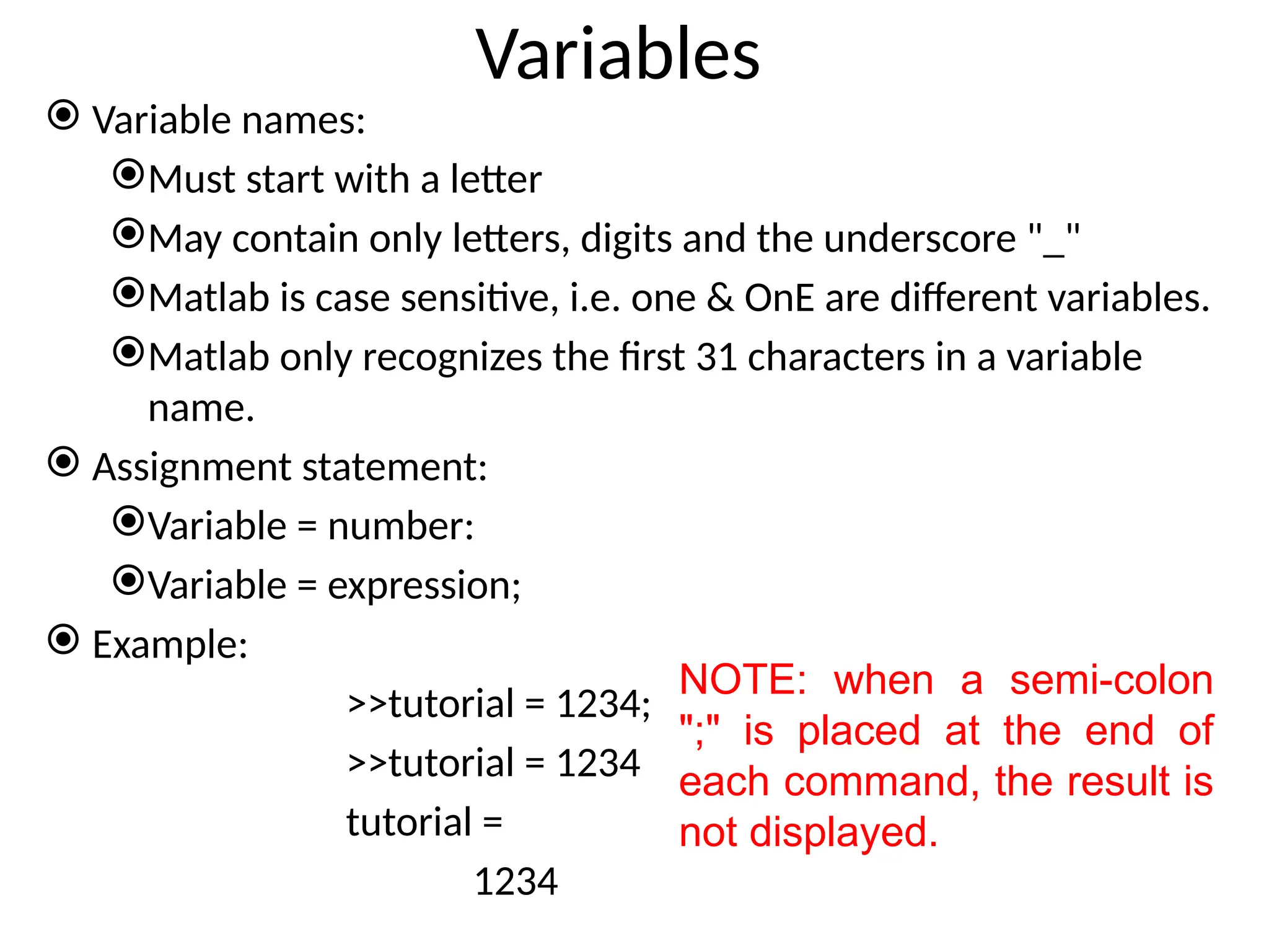
Variables  Variable names: Must start with a letter May contain only letters, digits and the underscore "_" Matlab is case sensitive, i.e. one & OnE are different variables. Matlab only recognizes the first 31 characters in a variable name.  Assignment statement: Variable = number: Variable = expression;  Example: >>tutorial = 1234; >>tutorial = 1234 tutorial = 1234 NOTE: when a semi-colon ";" is placed at the end of each command, the result is not displayed.

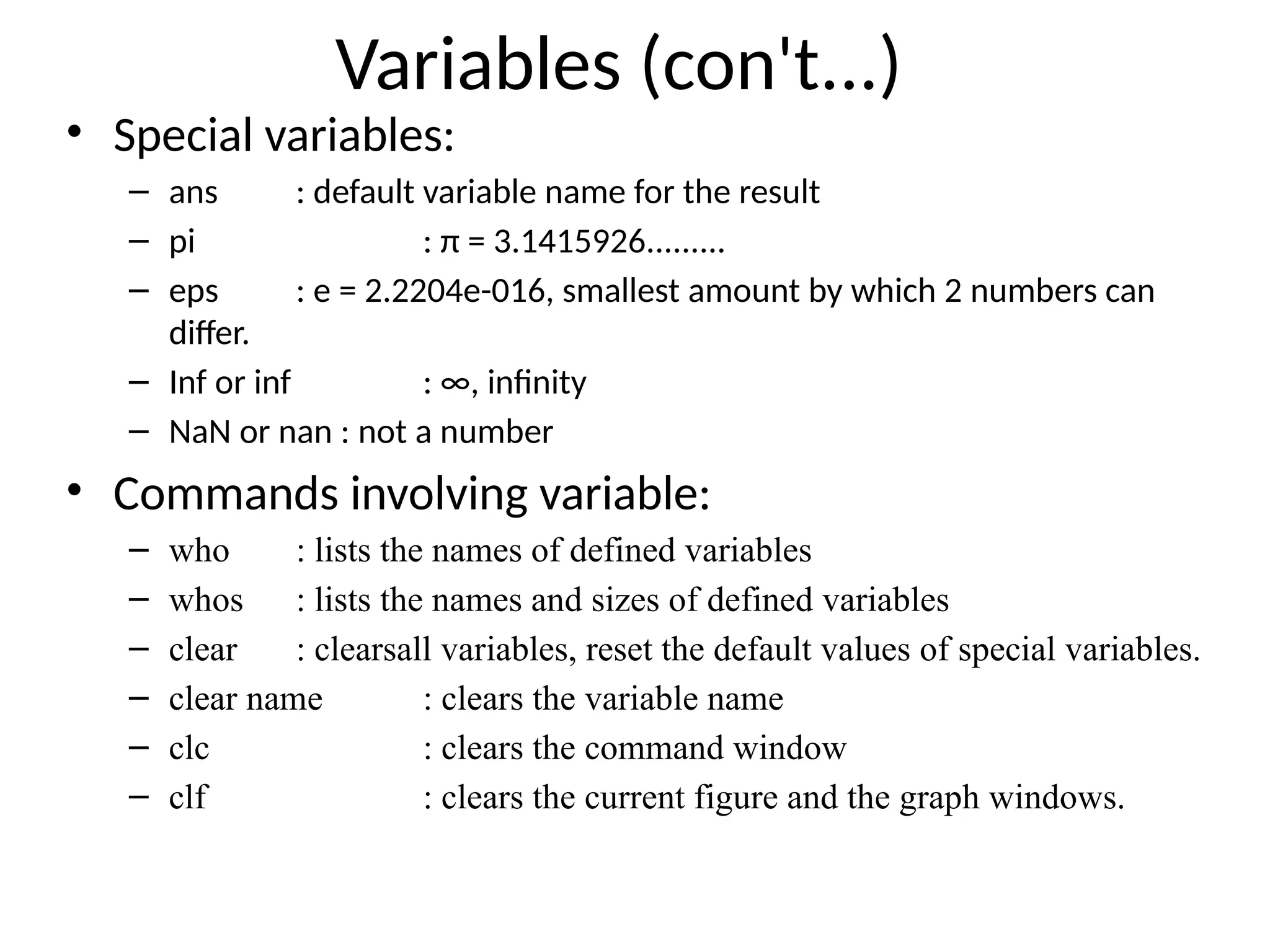
Variables (con't...) • Special variables: – ans : default variable name for the result – pi : π = 3.1415926......... – eps : e = 2.2204e-016, smallest amount by which 2 numbers can differ. – Inf or inf : ∞, infinity – NaN or nan : not a number • Commands involving variable: – who : lists the names of defined variables – whos : lists the names and sizes of defined variables – clear : clearsall variables, reset the default values of special variables. – clear name : clears the variable name – clc : clears the command window – clf : clears the current figure and the graph windows.

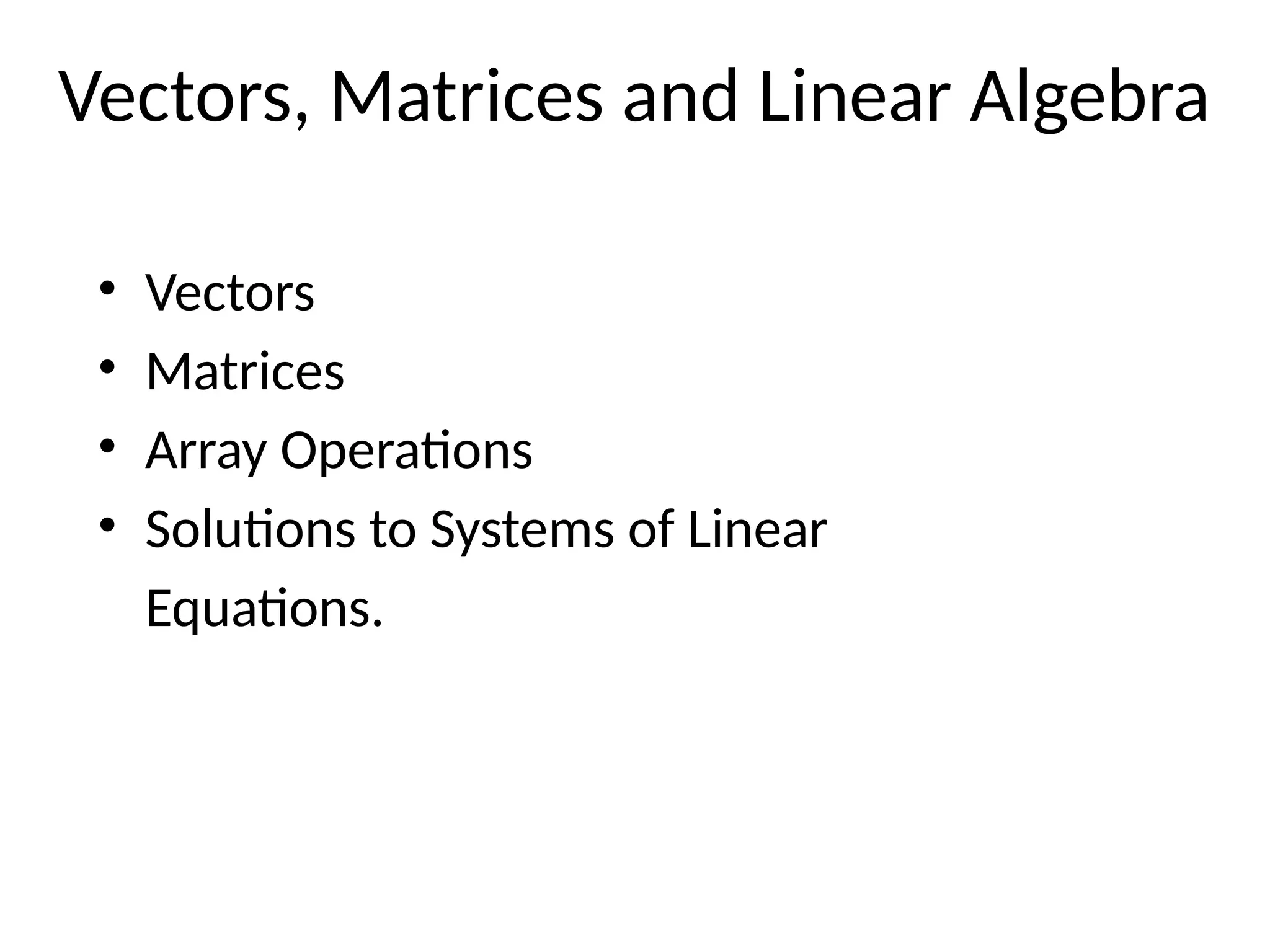
Vectors, Matrices and Linear Algebra • Vectors • Matrices • Array Operations • Solutions to Systems of Linear Equations.

Vectors  A row vector in MATLAB can be created by an explicit list, starting with a left bracket, entering the values separated by spaces (or commas) and vector with a right bracket.  A column vector can be created the same way, and the rows are separated by semicolons.  Example: >> x = [0 0.25*pi 0.5*pi 0.75*pi] x = 0 0.7854 1.5708 2.3582 3.0416 >> y = [0; 0.25*pi; 0.5*pi; 0.75*pi] y = 0 0.7854 1.5708 2.3562 3.1416 X is a row vector. Y is a column vector.

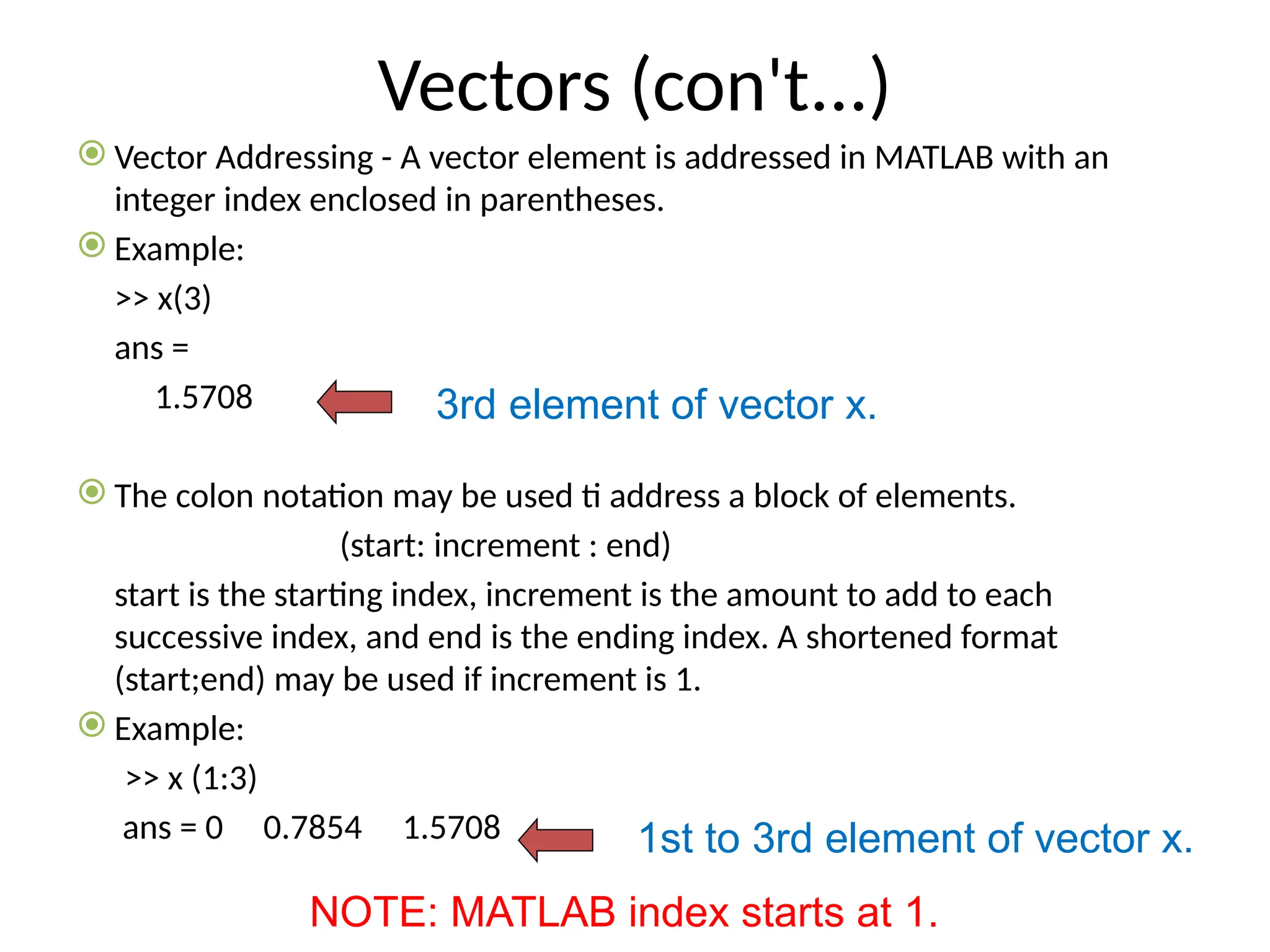
Vectors (con't...)  Vector Addressing - A vector element is addressed in MATLAB with an integer index enclosed in parentheses.  Example: >> x(3) ans = 1.5708  The colon notation may be used ti address a block of elements. (start: increment : end) start is the starting index, increment is the amount to add to each successive index, and end is the ending index. A shortened format (start;end) may be used if increment is 1.  Example: >> x (1:3) ans = 0 0.7854 1.5708 NOTE: MATLAB index starts at 1. 3rd element of vector x. 1st to 3rd element of vector x.

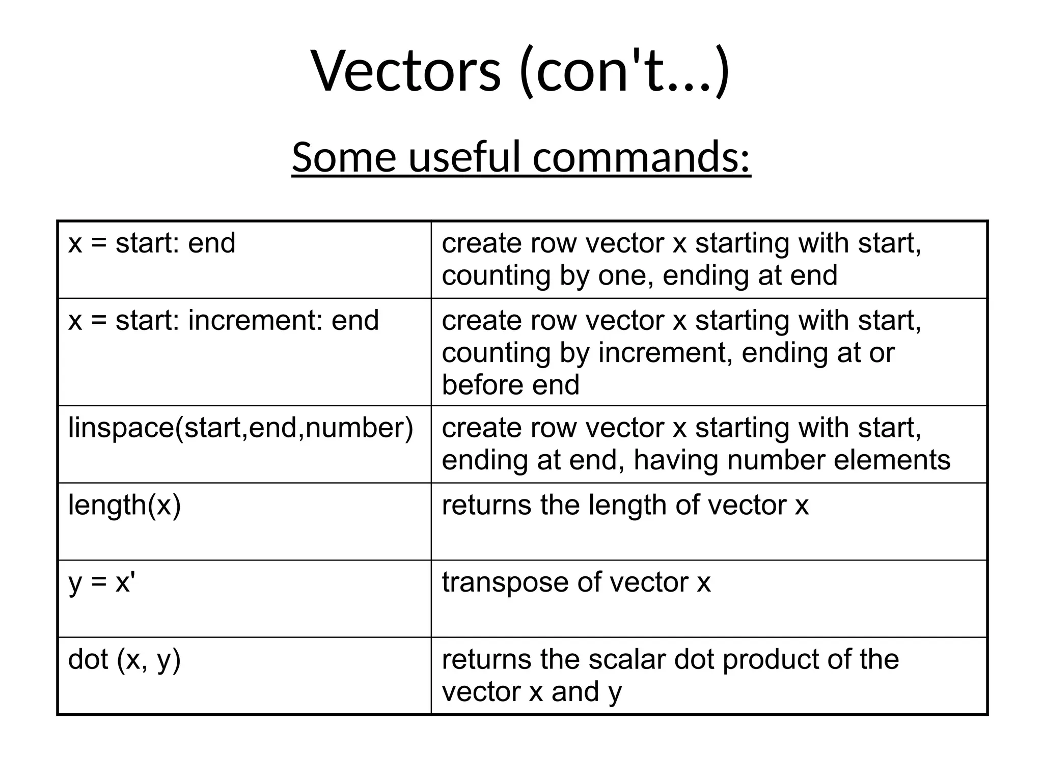
Vectors (con't...) Some useful commands: x = start: end create row vector x starting with start, counting by one, ending at end x = start: increment: end create row vector x starting with start, counting by increment, ending at or before end linspace(start,end,number) create row vector x starting with start, ending at end, having number elements length(x) returns the length of vector x y = x' transpose of vector x dot (x, y) returns the scalar dot product of the vector x and y

Matrices • A Matrix array is two-dimensional, having both multiple rows and multiple columns, similar to vector arrays: – it begins with [, and end with ] – spaces or commas are used to separate elements in a row. – semicolon or enter is used to separate rows. A is an m x n matrix. • Example: >> f = [ 1 2 3; 4 5 6] f = 1 2 3 4 5 6 >> h = [2 4 6 1 3 5] h = 2 4 6 1 3 5 The main diagonal                  mn m m m n n n a a a a a a a a a a a a a a a a A          3 2 1 3 33 32 31 2 23 22 21 1 13 12 11

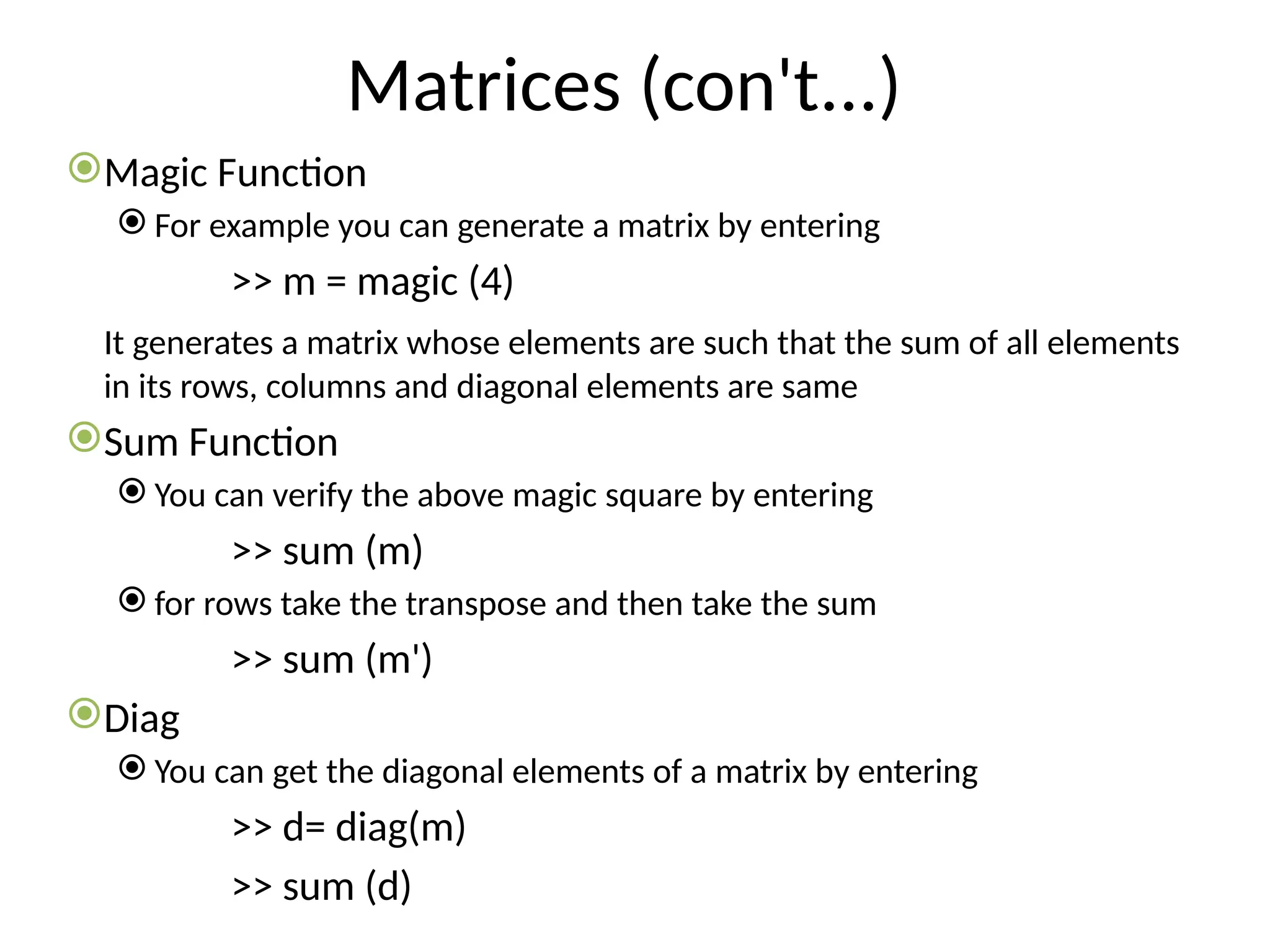
Matrices (con't...) Magic Function  For example you can generate a matrix by entering >> m = magic (4) It generates a matrix whose elements are such that the sum of all elements in its rows, columns and diagonal elements are same Sum Function  You can verify the above magic square by entering >> sum (m)  for rows take the transpose and then take the sum >> sum (m') Diag  You can get the diagonal elements of a matrix by entering >> d= diag(m) >> sum (d)

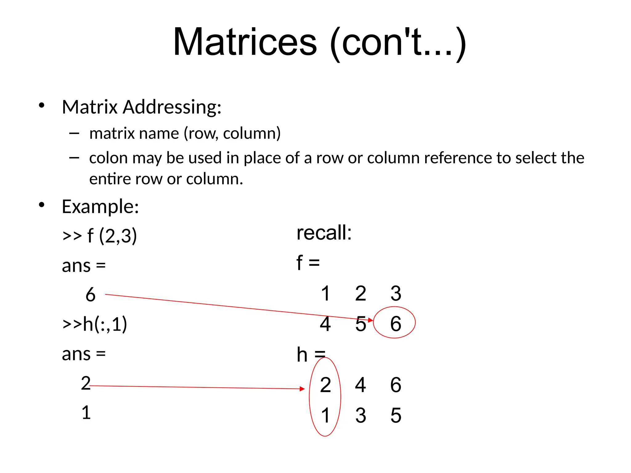
• Matrix Addressing: – matrix name (row, column) – colon may be used in place of a row or column reference to select the entire row or column. • Example: >> f (2,3) ans = 6 >>h(:,1) ans = 2 1 Matrices (con't...) recall: f = 1 2 3 4 5 6 h = 2 4 6 1 3 5

Matrices (con't...) Some useful commands: zeros(n) returns a n x n matrix of zeros zeros(m,n) returns a m x n matrix of zeros ones(n) returns a n x n matrix of ones ones(m,n) returns a m x n matrix of ones rand(n) returns a n x n matrix of random number rand(m,n) returns a m x n matrix of random number size (A) for a m x n matrix A, returns the row vector [m, n] containing the number of rows and columns in matrix. length(A) returns the large of the number of rows or columns in A.

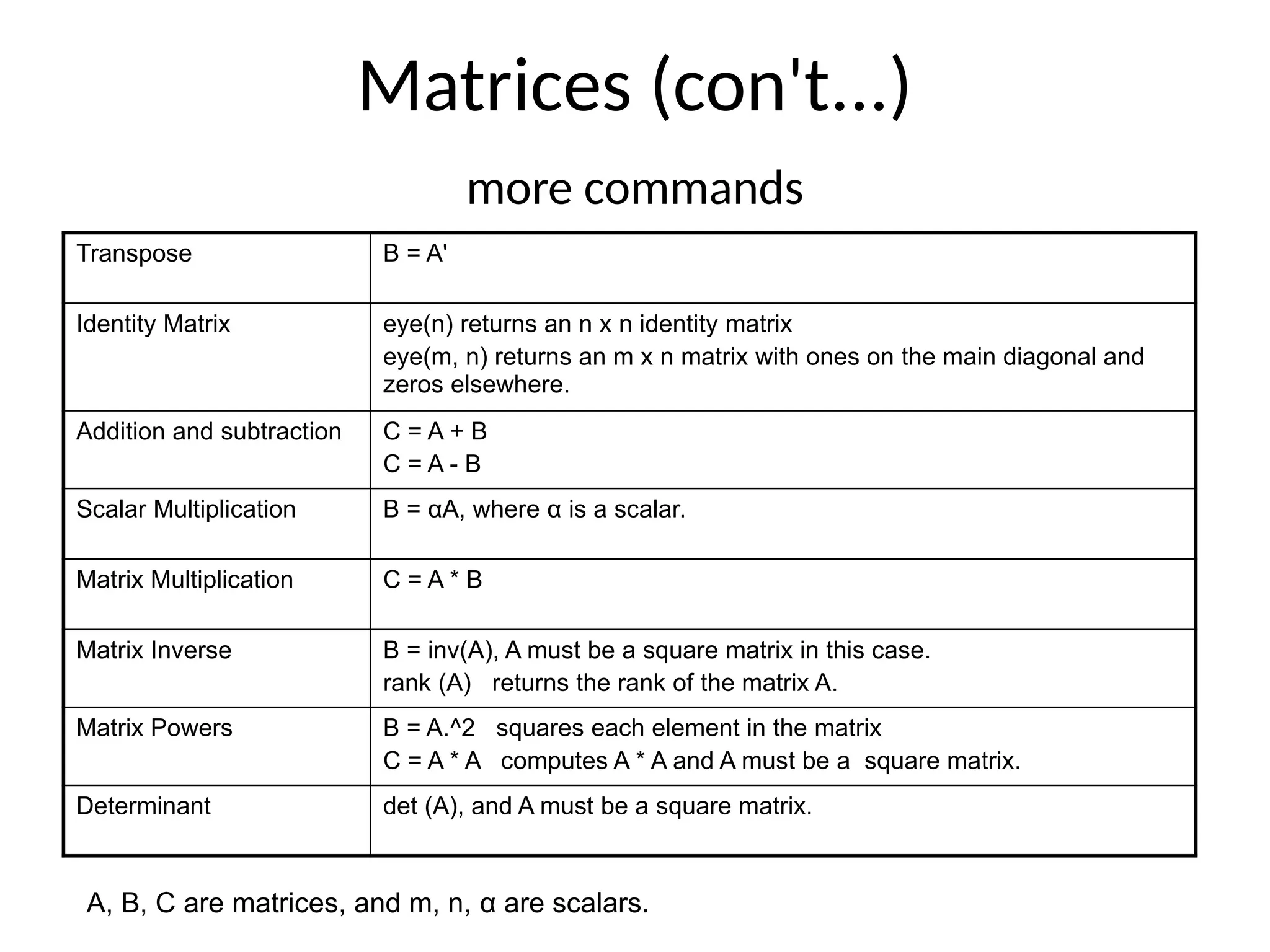
Matrices (con't...) more commands Transpose B = A' Identity Matrix eye(n) returns an n x n identity matrix eye(m, n) returns an m x n matrix with ones on the main diagonal and zeros elsewhere. Addition and subtraction C = A + B C = A - B Scalar Multiplication B = αA, where α is a scalar. Matrix Multiplication C = A * B Matrix Inverse B = inv(A), A must be a square matrix in this case. rank (A) returns the rank of the matrix A. Matrix Powers B = A.^2 squares each element in the matrix C = A * A computes A * A and A must be a square matrix. Determinant det (A), and A must be a square matrix. A, B, C are matrices, and m, n, α are scalars.

Array Operations • Scalar-Array Mathematics For addition, subtraction, multiplication, and division of an array by a scalar simply apply the operations to all elements if the array. • Example: >> f = [1 2; 3 4] f = 1 2 3 4 >> g = 2*f - 1 g = 1 3 5 7 Each element in the array f is multiplied by 2, then subtracted by 1.

Array Operations (con’t…) • Element-by-Element Array-Array Mathematics. Operation Algebraic Form MATLAB Addition a + b a + b Subtraction a – b a – b Multiplication a x b a.*b Division a ÷ b a./b Exponentiation ab a.^b  Example: >> x = [1 2 3 ]; >> y = [4 5 6 ]; >> z = x.*y z = 4 10 18 Each element in x is multiplied by the corresponding element in y.

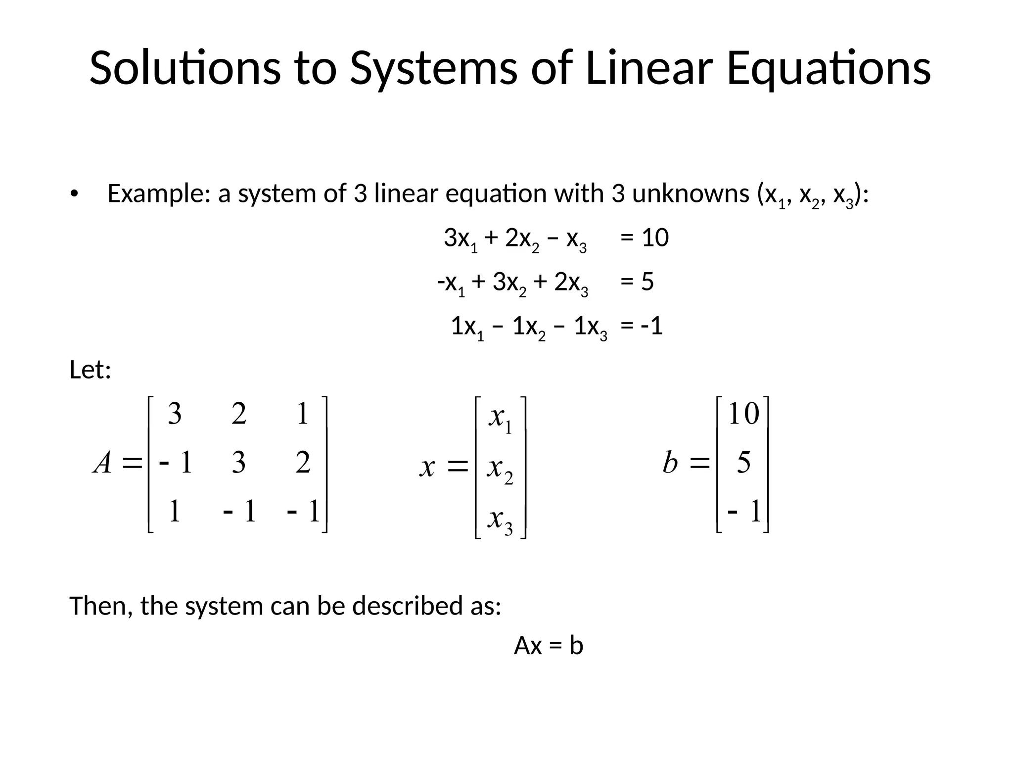
Solutions to Systems of Linear Equations • Example: a system of 3 linear equation with 3 unknowns (x1, x2, x3): 3x1 + 2x2 – x3 = 10 -x1 + 3x2 + 2x3 = 5 1x1 – 1x2 – 1x3 = -1 Let: Then, the system can be described as: Ax = b               1 1 1 2 3 1 1 2 3 A            3 2 1 x x x x             1 5 10 b

Solutions to Systems of Linear Equations (con’t…) • Solution by Matrix Inverse: Ax = b A-1 Ax = A-1 b X = A-1 b • MATLAB: >> A = [3 2 -1; -1 3 2; 1 -1 -1]; >> b = [10 5 -1]; >> x = inv(A)*b x = -2.0000 5.0000 -6.0000  Solution by Matrix Division: The solution to the equation Ax = b can be computed using left division.  MATLAB: >> A = [3 2 -1; -1 3 2; 1 -1 -1]; >> b = [10 5 -1]; >> x = Ab x = -2.0000 5.0000 -6.0000 NOTE: left division: Ab b ÷ A right division: x/y x ÷ y

Plotting  For more information on 2-D plotting, type help graph2d  Plotting a point:  >> plot(variablename, ‘symbol’)  Example : Complex number  >> z = 1 + 0.5j;  >> plot(z,’ . ’) Command Description Axis([xmin xmax ymin ymax]) Define minimum & maximum values of the axes axis square Produce a square plot axis equal Equal scaling factors for both axes axis normal Turn off axis square, equal axis (auto) Return the axis to defaults The function plot() creates a graphics window, called a Figure window, and named by default “Figure No.1” 0 0.2 0.4 0.6 0.8 1 1.2 1.4 1.6 1.8 2 -0.5 0 0.5 1 1.5

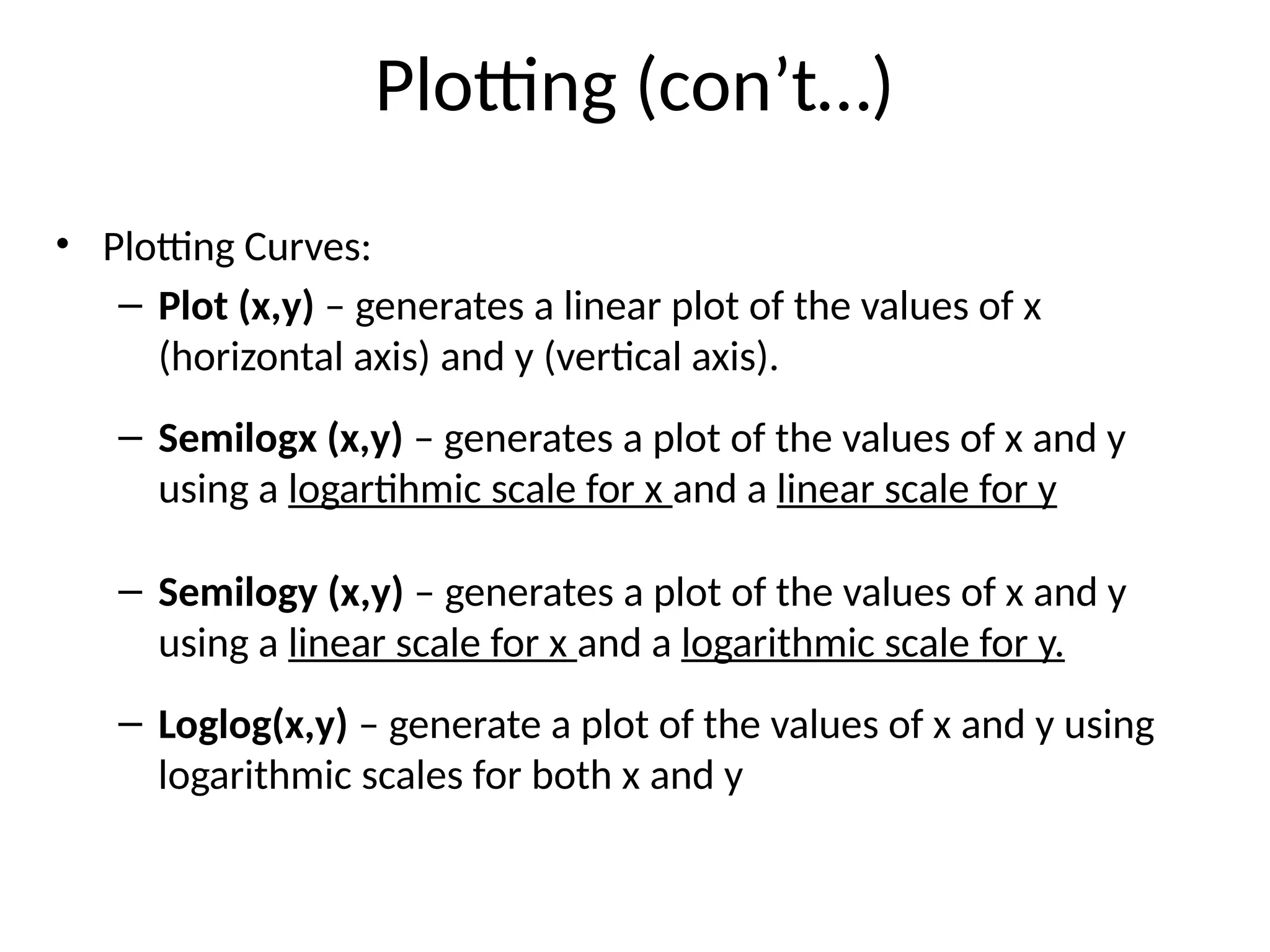
Plotting (con’t…) • Plotting Curves: – Plot (x,y) – generates a linear plot of the values of x (horizontal axis) and y (vertical axis). – Semilogx (x,y) – generates a plot of the values of x and y using a logartihmic scale for x and a linear scale for y – Semilogy (x,y) – generates a plot of the values of x and y using a linear scale for x and a logarithmic scale for y. – Loglog(x,y) – generate a plot of the values of x and y using logarithmic scales for both x and y

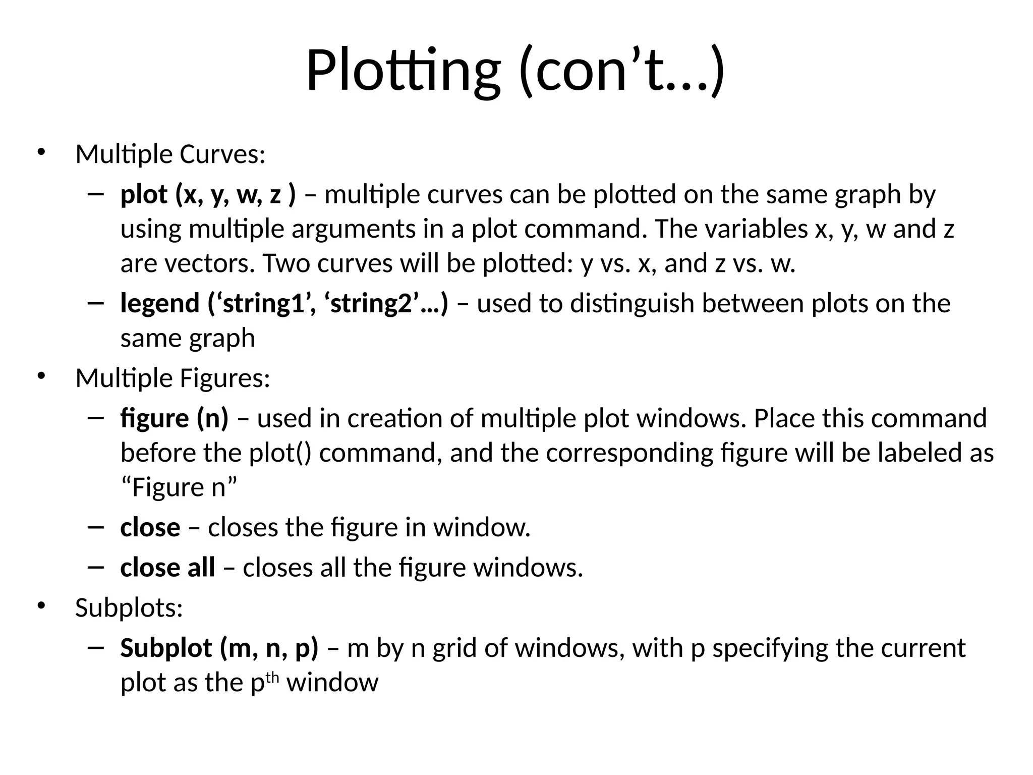
Plotting (con’t…) • Multiple Curves: – plot (x, y, w, z ) – multiple curves can be plotted on the same graph by using multiple arguments in a plot command. The variables x, y, w and z are vectors. Two curves will be plotted: y vs. x, and z vs. w. – legend (‘string1’, ‘string2’…) – used to distinguish between plots on the same graph • Multiple Figures: – figure (n) – used in creation of multiple plot windows. Place this command before the plot() command, and the corresponding figure will be labeled as “Figure n” – close – closes the figure in window. – close all – closes all the figure windows. • Subplots: – Subplot (m, n, p) – m by n grid of windows, with p specifying the current plot as the pth window

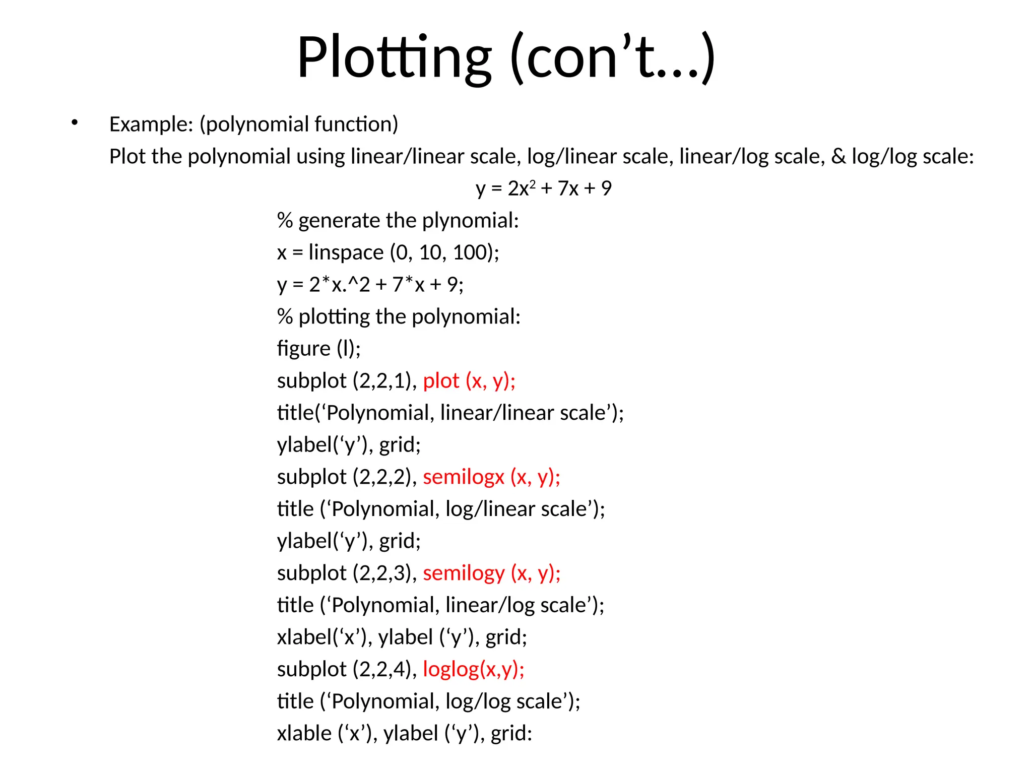
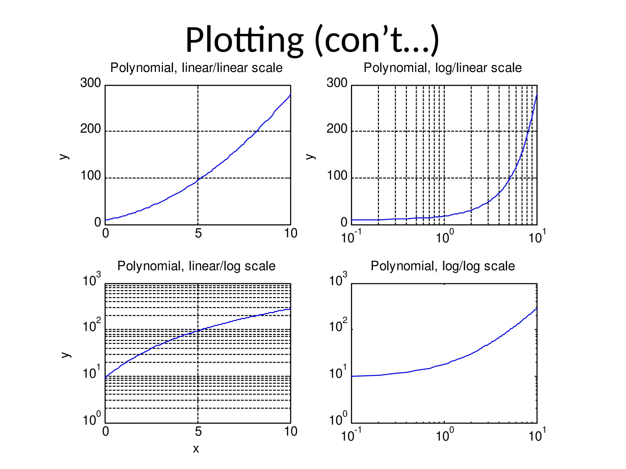
Plotting (con’t…) • Example: (polynomial function) Plot the polynomial using linear/linear scale, log/linear scale, linear/log scale, & log/log scale: y = 2x2 + 7x + 9 % generate the plynomial: x = linspace (0, 10, 100); y = 2*x.^2 + 7*x + 9; % plotting the polynomial: figure (l); subplot (2,2,1), plot (x, y); title(‘Polynomial, linear/linear scale’); ylabel(‘y’), grid; subplot (2,2,2), semilogx (x, y); title (‘Polynomial, log/linear scale’); ylabel(‘y’), grid; subplot (2,2,3), semilogy (x, y); title (‘Polynomial, linear/log scale’); xlabel(‘x’), ylabel (‘y’), grid; subplot (2,2,4), loglog(x,y); title (‘Polynomial, log/log scale’); xlable (‘x’), ylabel (‘y’), grid:

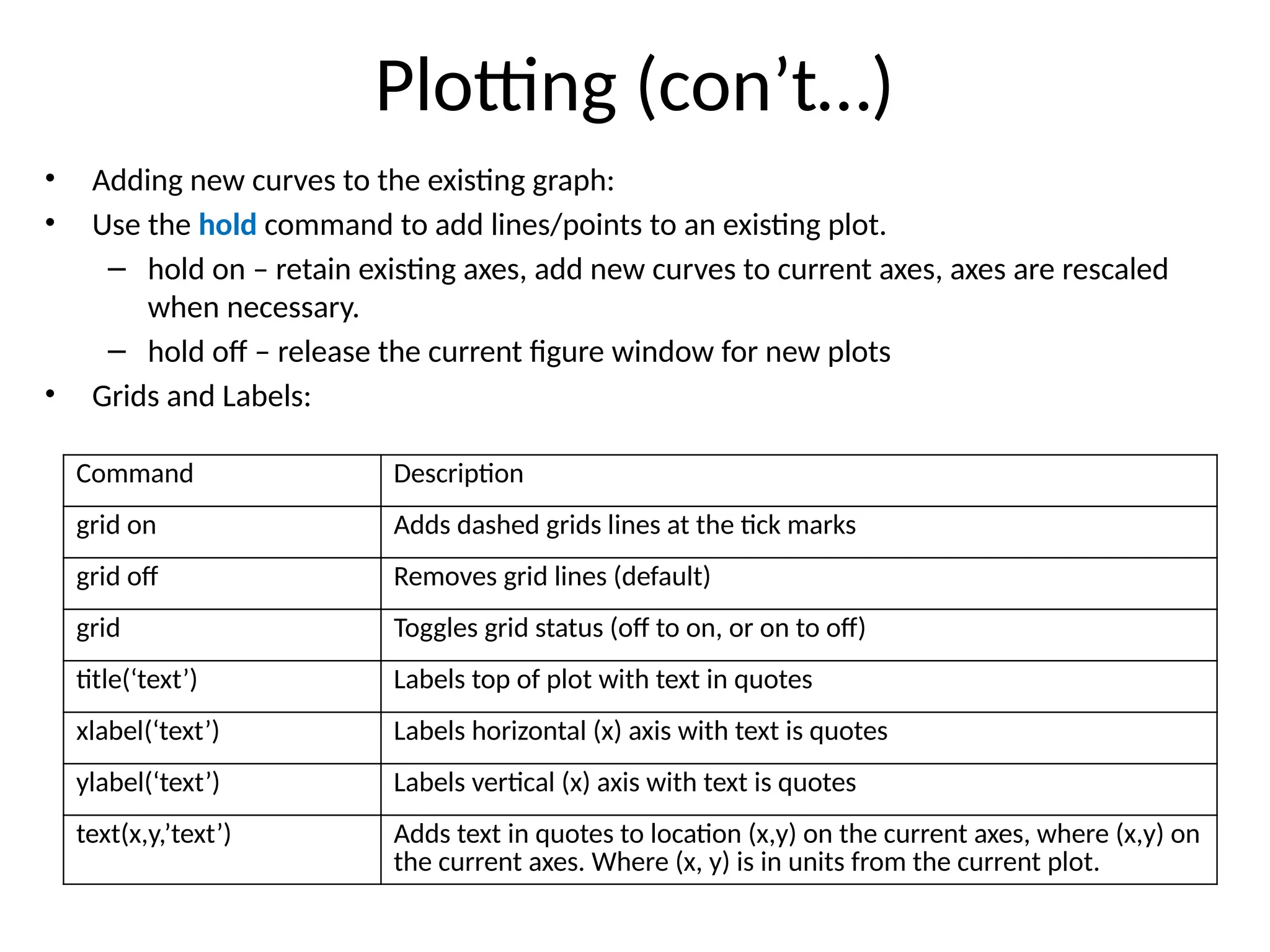
Plotting (con’t…) 0 5 10 0 100 200 300 Polynomial, linear/linear scale y 10 -1 10 0 10 1 0 100 200 300 Polynomial, log/linear scale y 0 5 10 10 0 10 1 10 2 10 3 Polynomial, linear/log scale x y 10 -1 10 0 10 1 10 0 10 1 10 2 10 3 Polynomial, log/log scale

Plotting (con’t…) • Adding new curves to the existing graph: • Use the hold command to add lines/points to an existing plot. – hold on – retain existing axes, add new curves to current axes, axes are rescaled when necessary. – hold off – release the current figure window for new plots • Grids and Labels: Command Description grid on Adds dashed grids lines at the tick marks grid off Removes grid lines (default) grid Toggles grid status (off to on, or on to off) title(‘text’) Labels top of plot with text in quotes xlabel(‘text’) Labels horizontal (x) axis with text is quotes ylabel(‘text’) Labels vertical (x) axis with text is quotes text(x,y,’text’) Adds text in quotes to location (x,y) on the current axes, where (x,y) on the current axes. Where (x, y) is in units from the current plot.

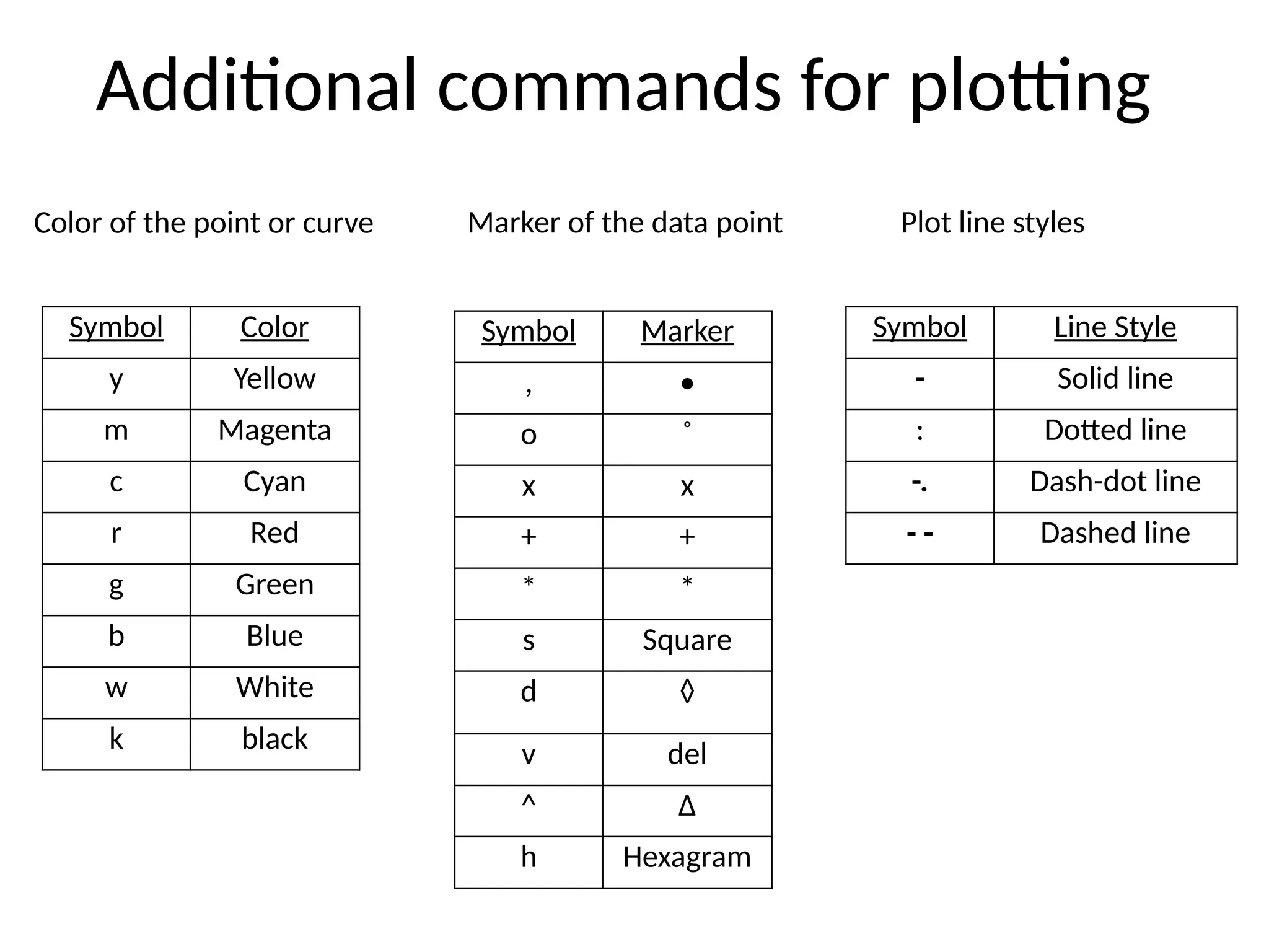
Additional commands for plotting Color of the point or curve Marker of the data point Plot line styles Symbol Color y Yellow m Magenta c Cyan r Red g Green b Blue w White k black Symbol Marker , • o ˚ x x + + * * s Square d ◊ v del ^ Δ h Hexagram Symbol Line Style - Solid line : Dotted line -. Dash-dot line - - Dashed line

Introduction to MATLAB Programming for Engineers

More Related Content

Similar to Introduction to MATLAB Programming for Engineers

Recently uploaded

Introduction to MATLAB Programming for Engineers