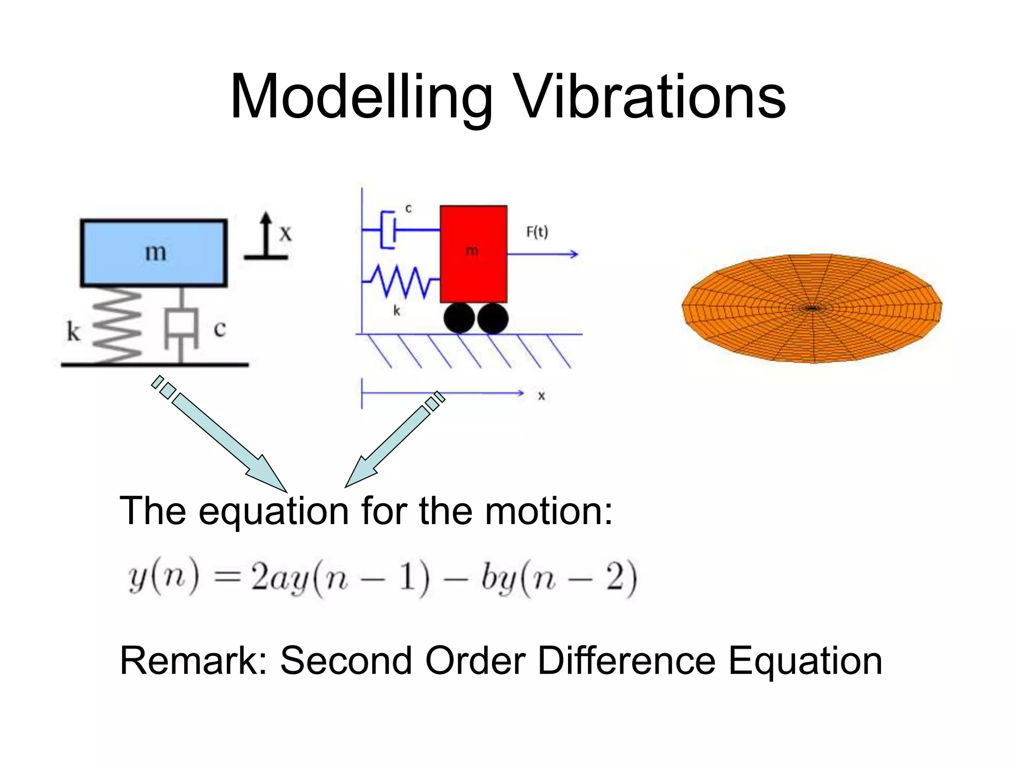
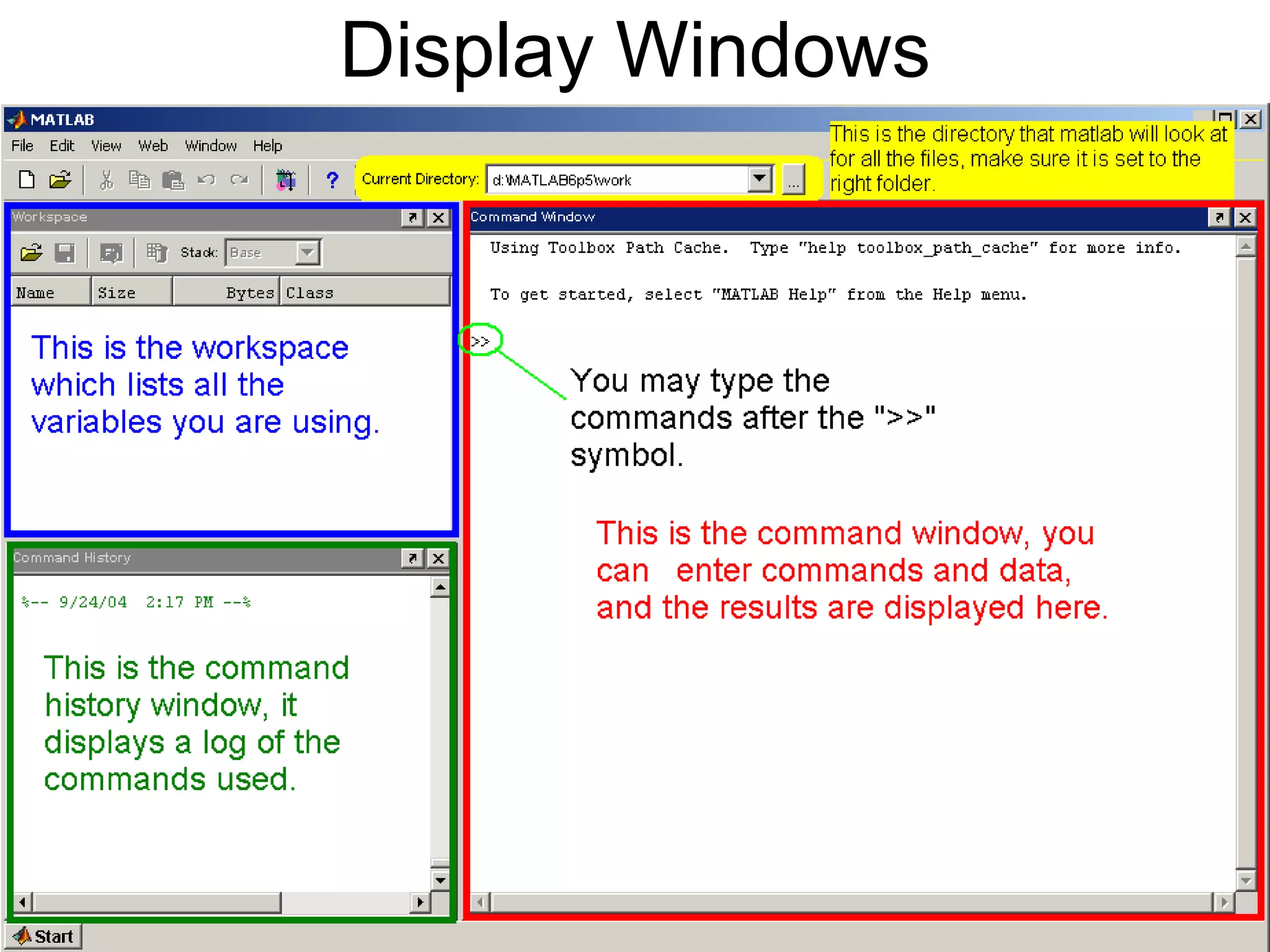
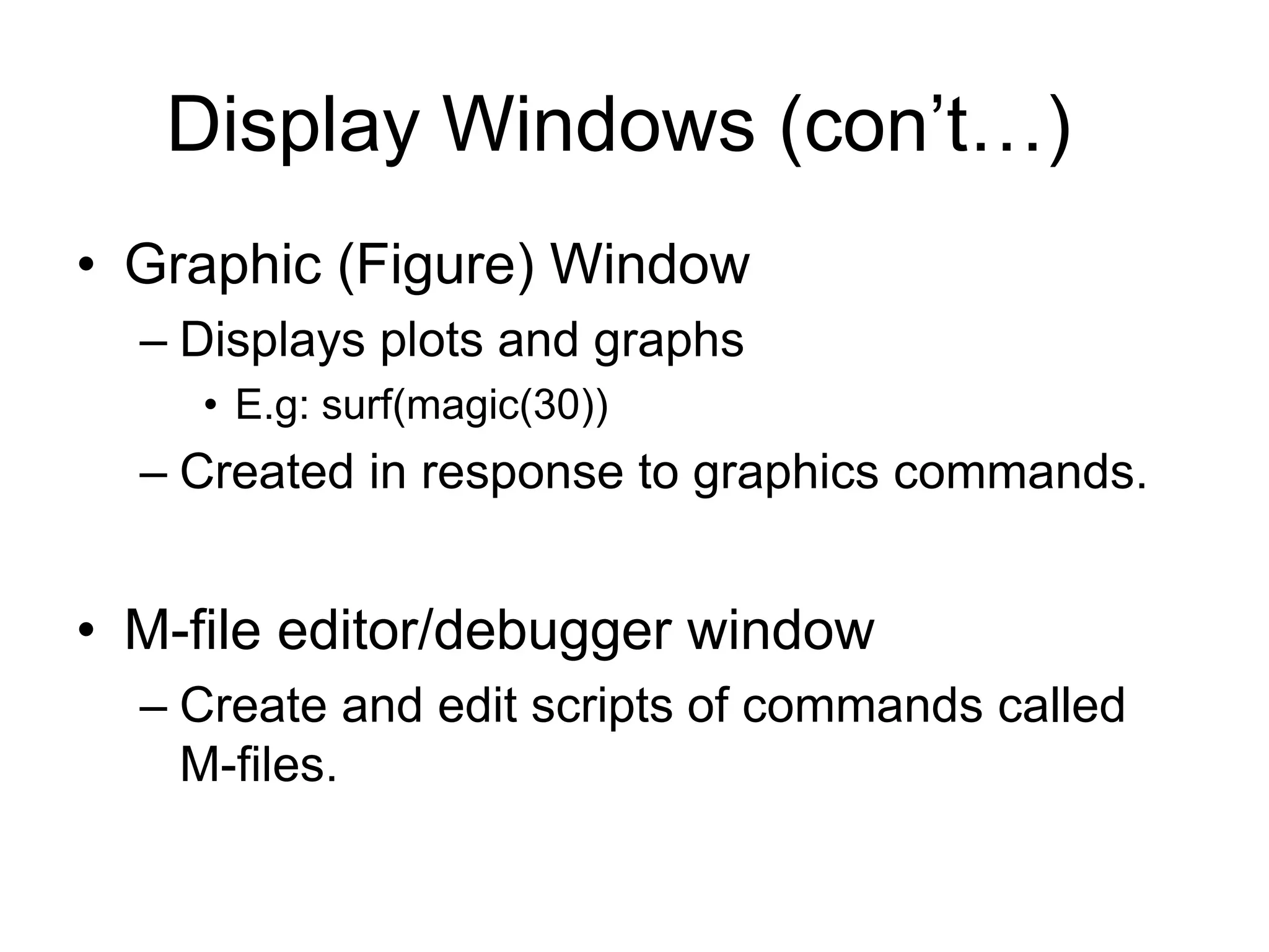
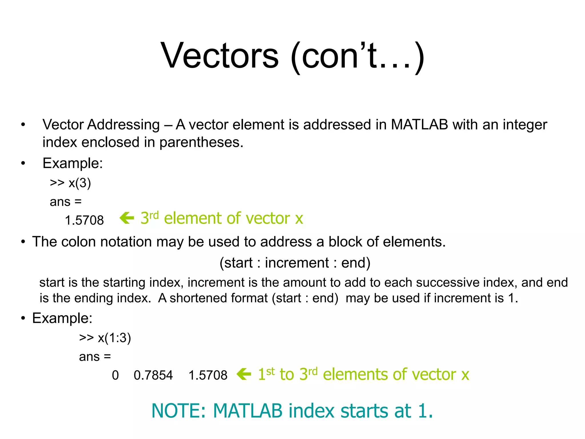
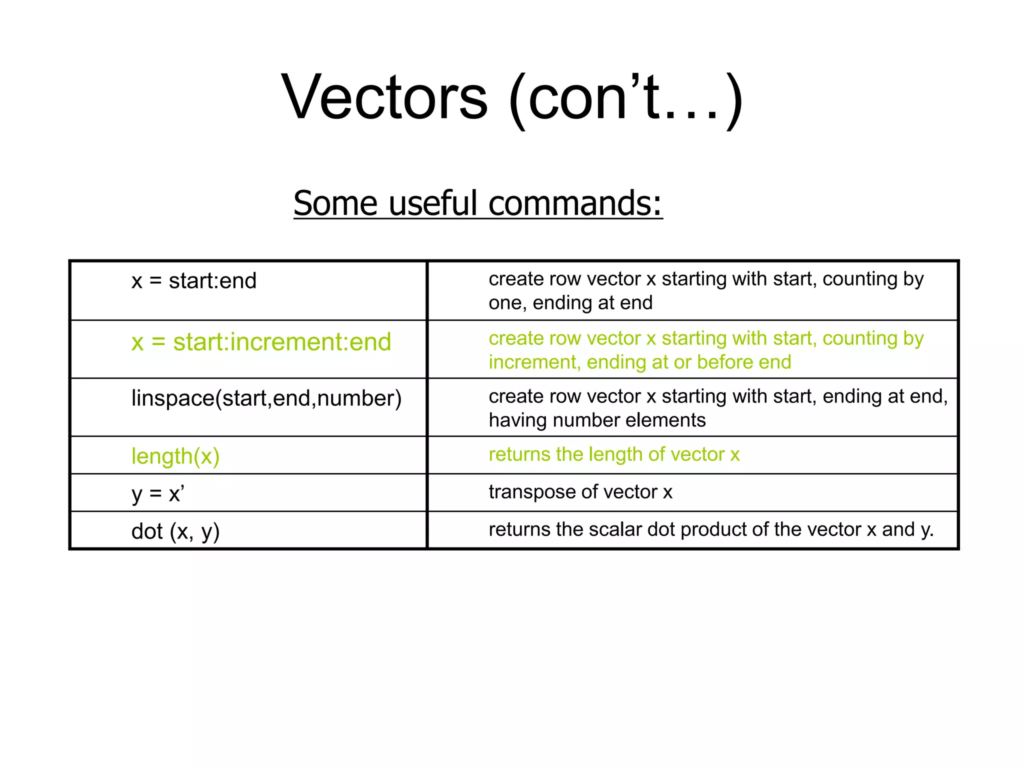
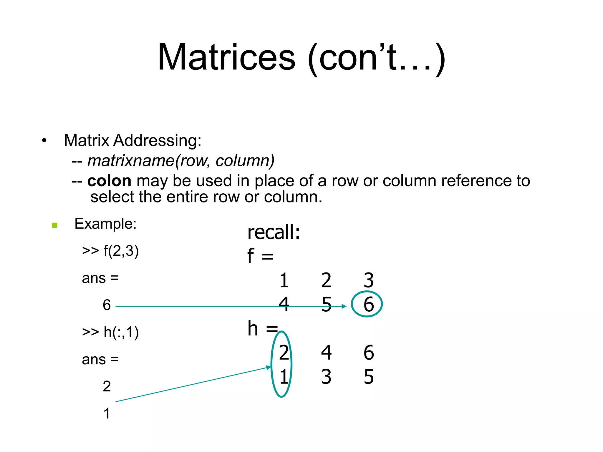
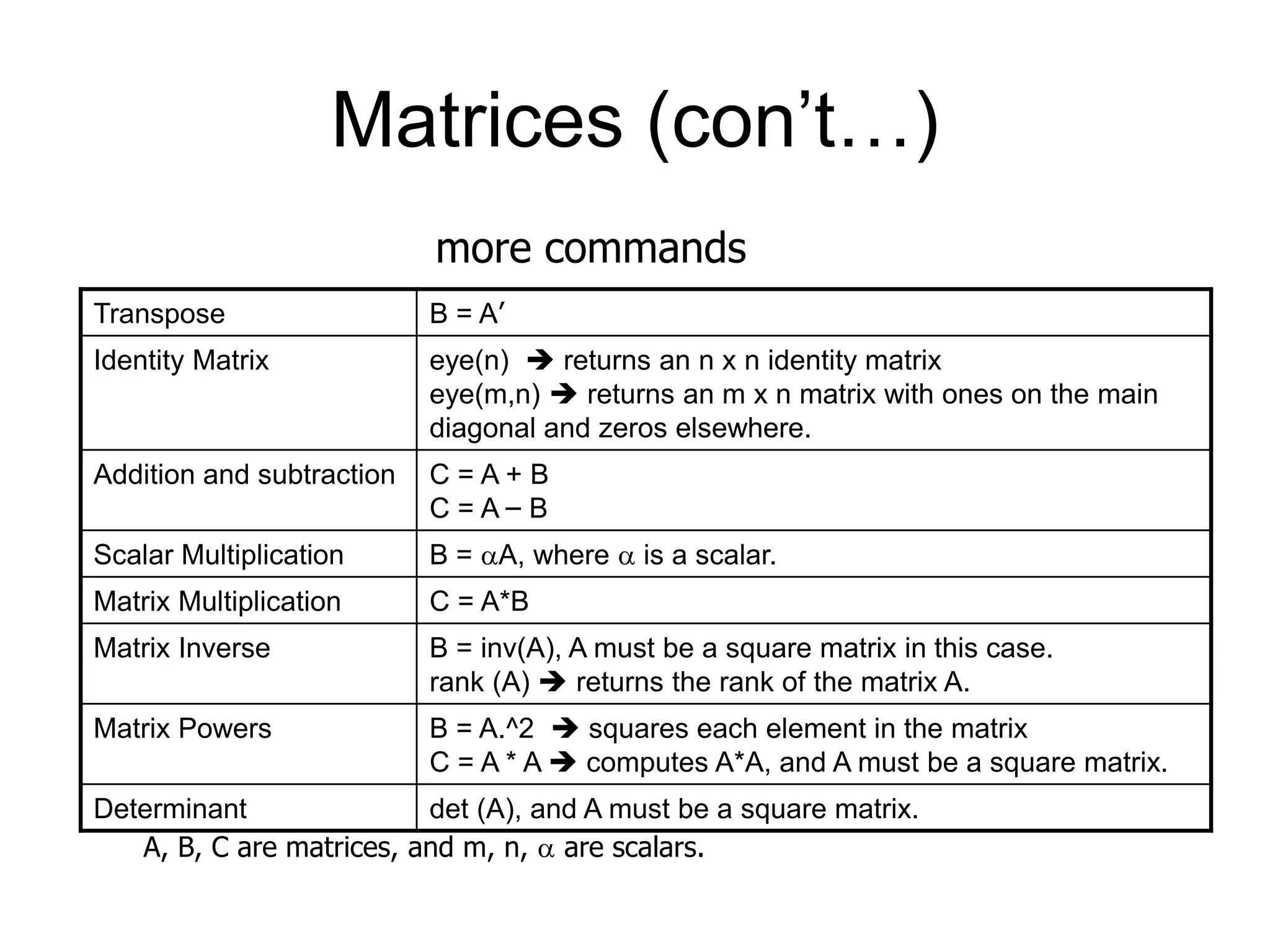
This document provides an introduction and overview of MATLAB. It discusses the MATLAB environment and windows, how to get help, variables, vectors, matrices, linear algebra, flow control, plotting, and modeling vibrations. The key topics covered include the command window, M-file editor, help commands, assigning variables, addressing vectors and matrices, common matrix operations, if/else and loop statements, generating plots, and solving second order difference equations to model vibrations.
![Vectors Example: >> x = [ 0 0.25*pi 0.5*pi 0.75*pi pi ] x = 0 0.7854 1.5708 2.3562 3.1416 >> y = [ 0; 0.25*pi; 0.5*pi; 0.75*pi; pi ] y = 0 0.7854 1.5708 2.3562 3.1416 x is a row vector. y is a column vector.](https://image.slidesharecdn.com/matlabtutorial-220811073052-8ae1a074/75/matlab_tutorial-ppt-9-2048.jpg)
![Matrices A is an m x n matrix. A Matrix array is two-dimensional, having both multiple rows and multiple columns, similar to vector arrays: it begins with [, and end with ] spaces or commas are used to separate elements in a row semicolon or enter is used to separate rows. •Example: •>> f = [ 1 2 3; 4 5 6] f = 1 2 3 4 5 6 the main diagonal](https://image.slidesharecdn.com/matlabtutorial-220811073052-8ae1a074/75/matlab_tutorial-ppt-12-2048.jpg)
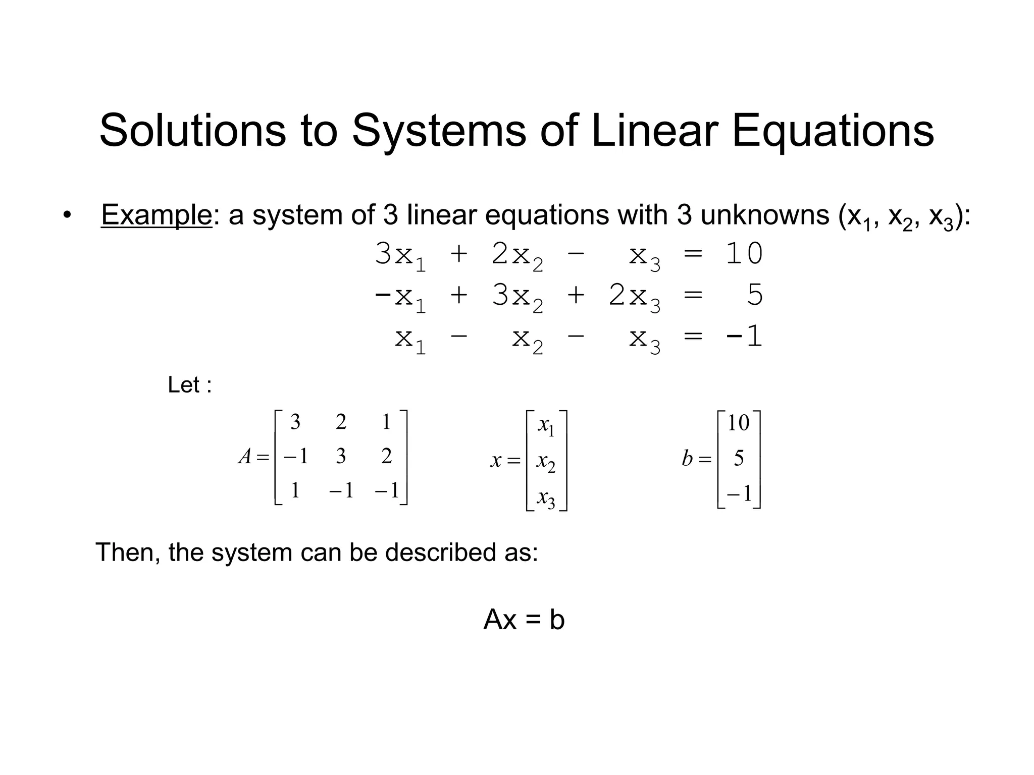
![Solutions to Systems of Linear Equations (con’t…) • Solution by Matrix Inverse: Ax = b A-1Ax = A-1b x = A-1b • MATLAB: >> A = [ 3 2 -1; -1 3 2; 1 -1 -1]; >> b = [ 10; 5; -1]; >> x = inv(A)*b x = -2.0000 5.0000 -6.0000 Answer: x1 = -2, x2 = 5, x3 = -6 • Solution by Matrix Division: The solution to the equation Ax = b can be computed using left division. Answer: x1 = -2, x2 = 5, x3 = -6 NOTE: left division: Ab b A right division: x/y x y MATLAB: >> A = [ 3 2 -1; -1 3 2; 1 -1 -1]; >> b = [ 10; 5; -1]; >> x = Ab x = -2.0000 5.0000 -6.0000](https://image.slidesharecdn.com/matlabtutorial-220811073052-8ae1a074/75/matlab_tutorial-ppt-16-2048.jpg)
![Visualization: Plotting • Example: >> s = linspace (-5, 5, 100); >> coeff = [ 1 3 3 1]; >> A = polyval (coeff, s); >> plot (s, A), >> xlabel ('s') >> ylabel ('A(s)') A(s) = s3 + 3s2 + 3s + 1](https://image.slidesharecdn.com/matlabtutorial-220811073052-8ae1a074/75/matlab_tutorial-ppt-20-2048.jpg)