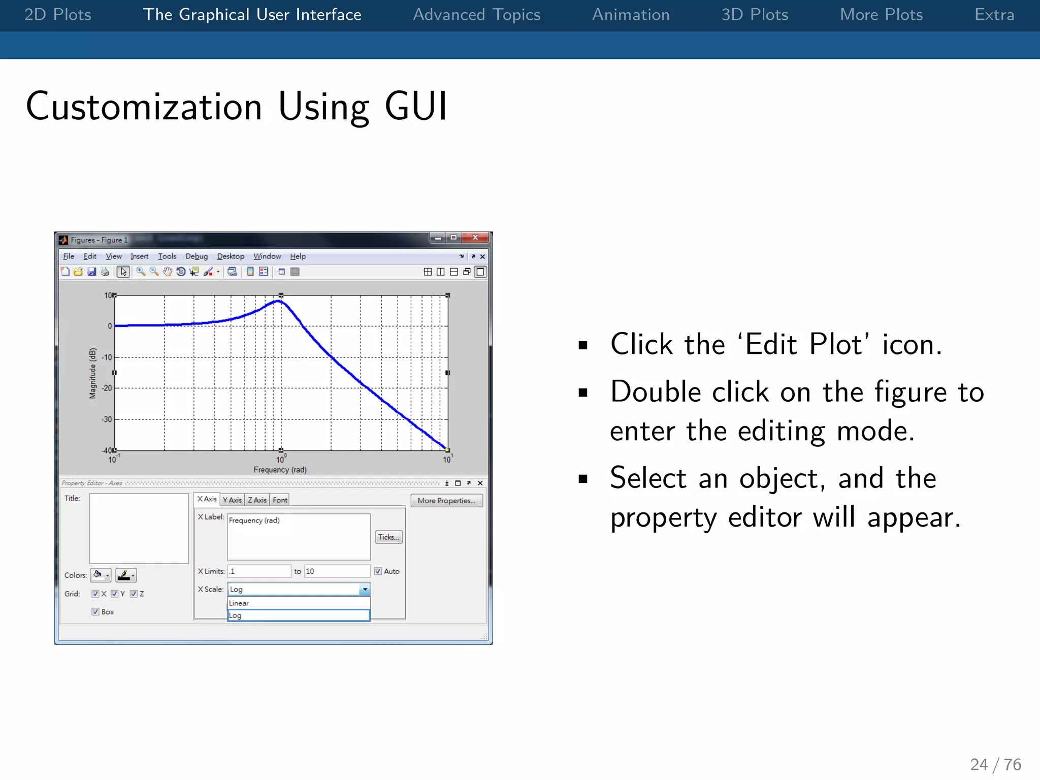
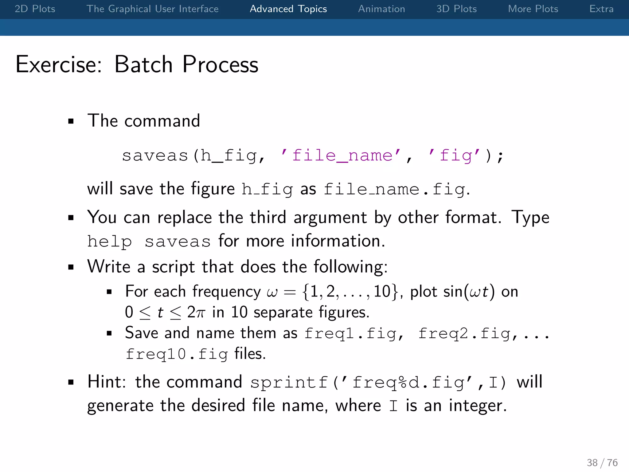
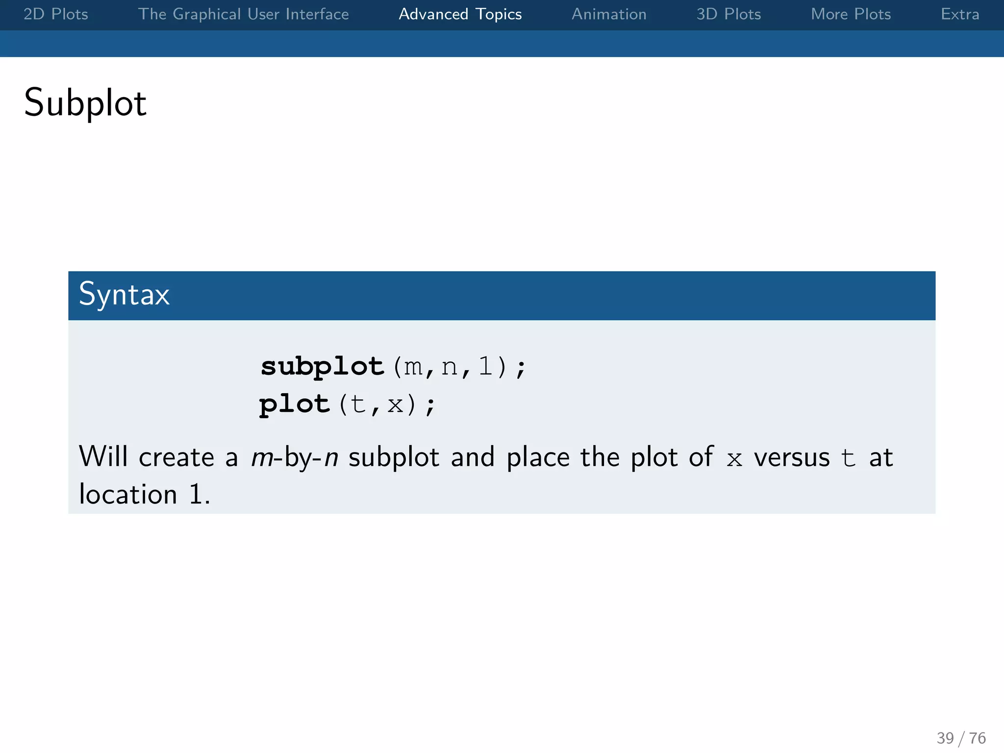
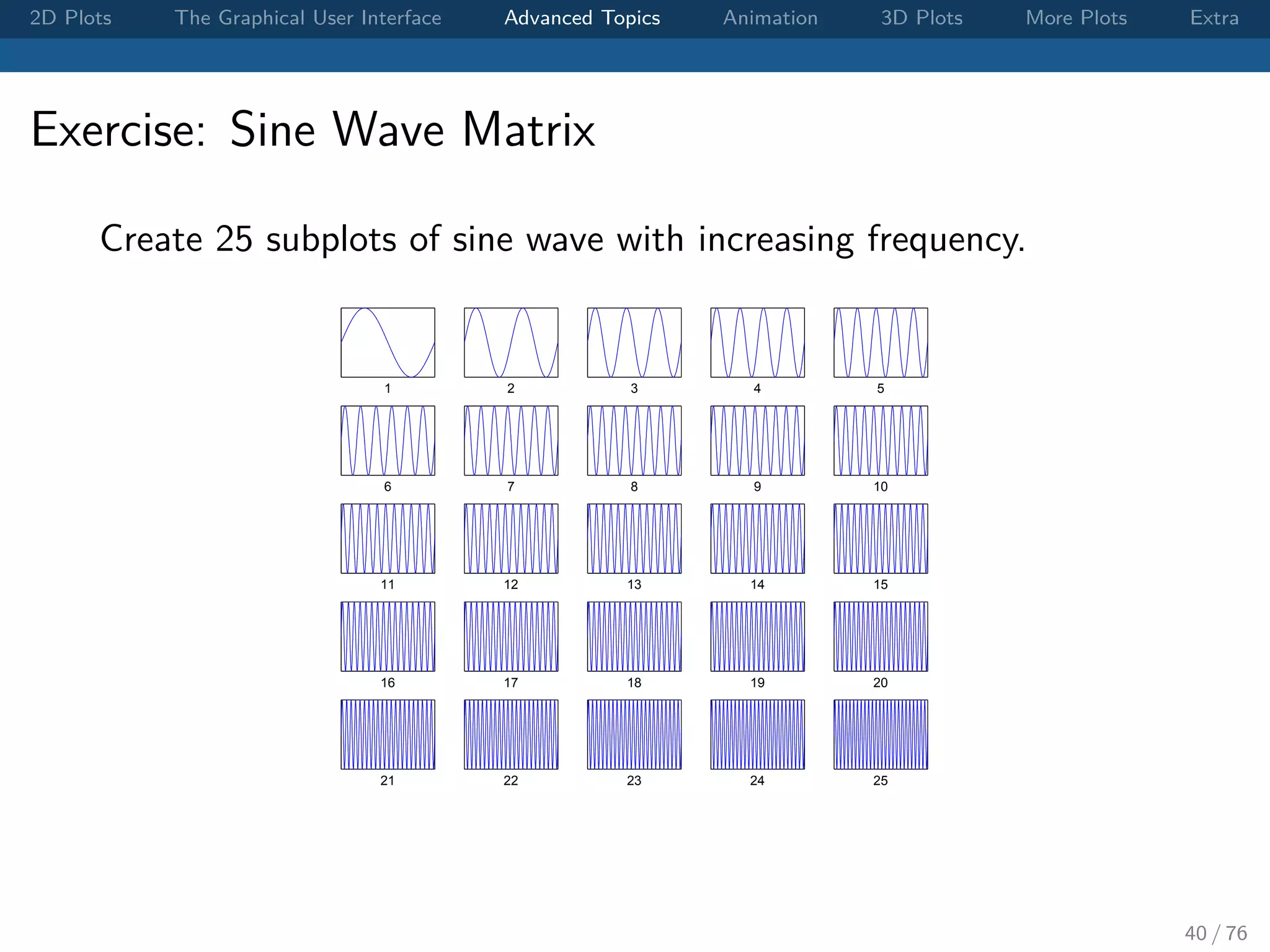
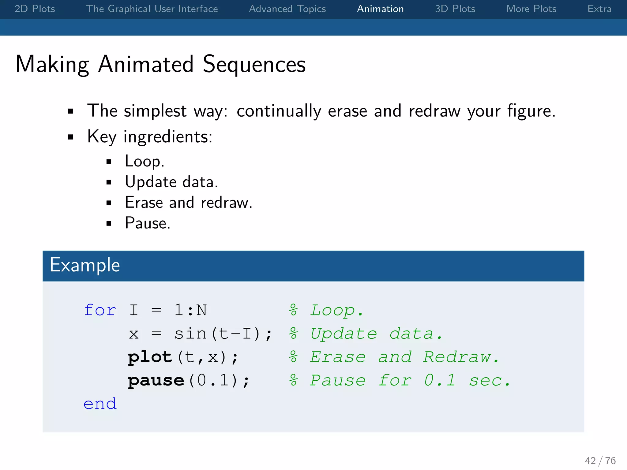
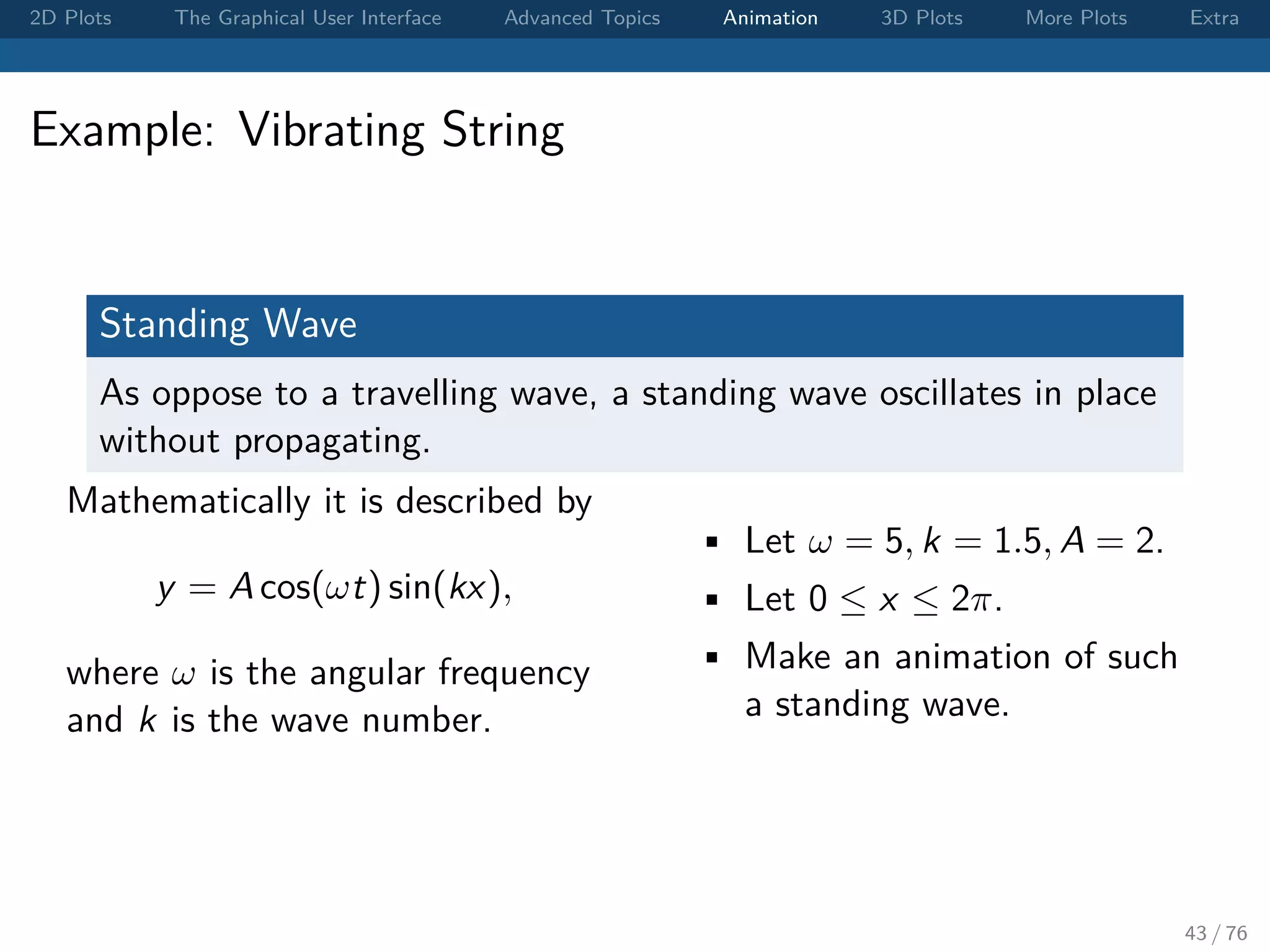
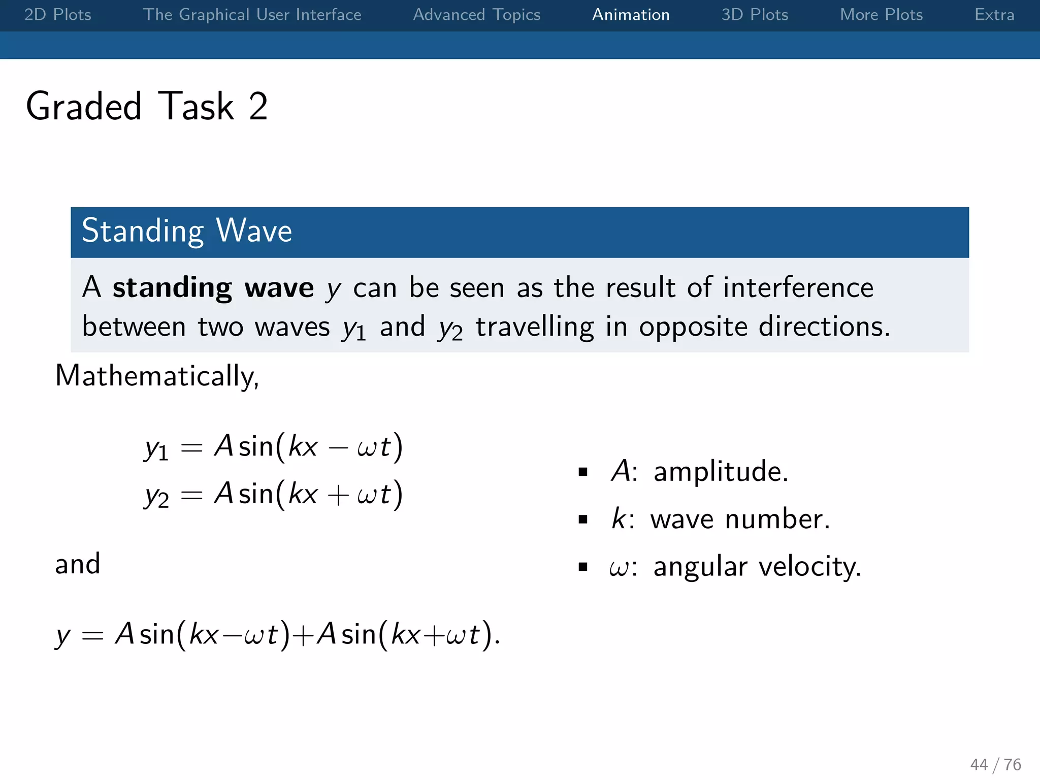
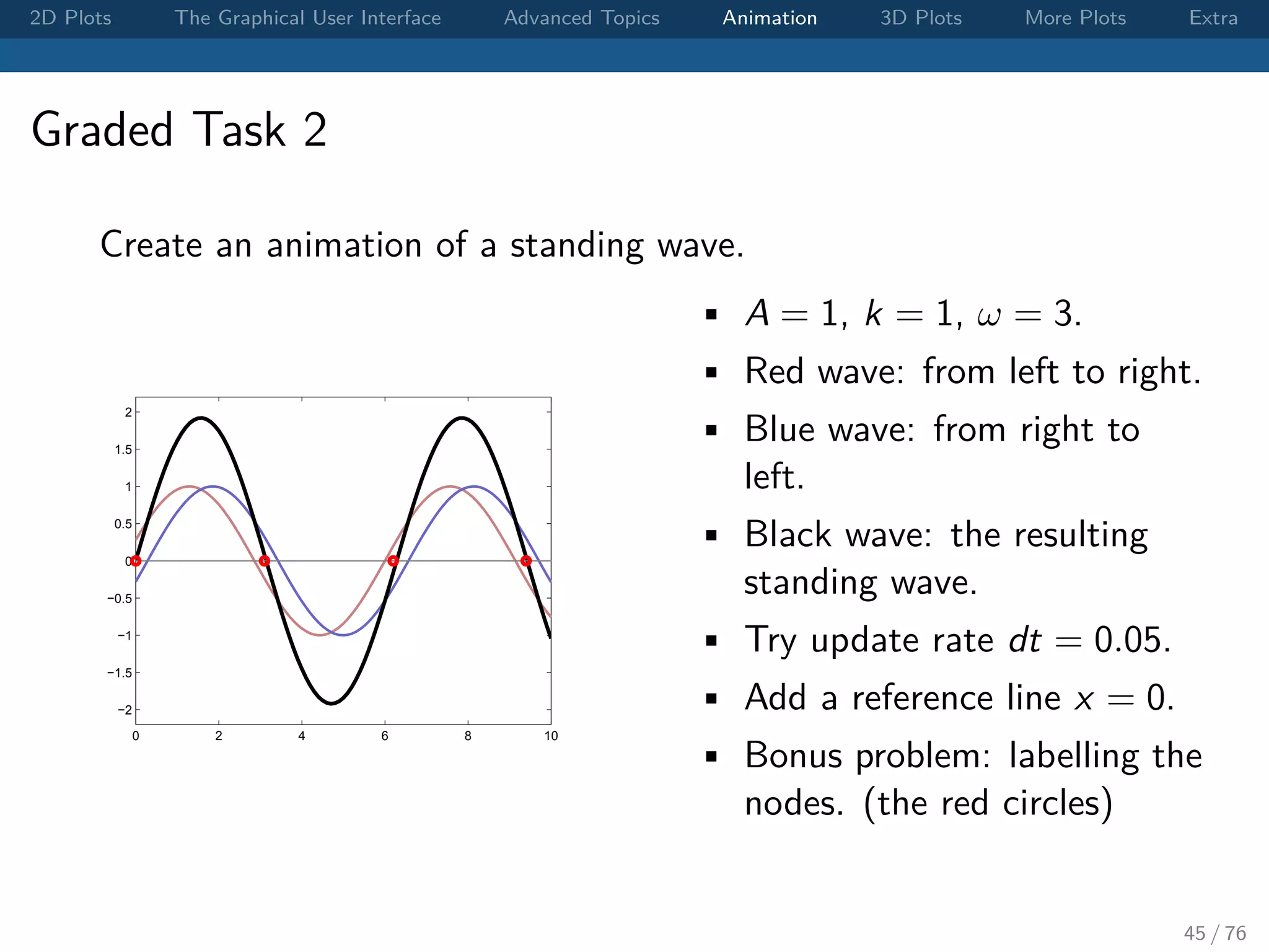
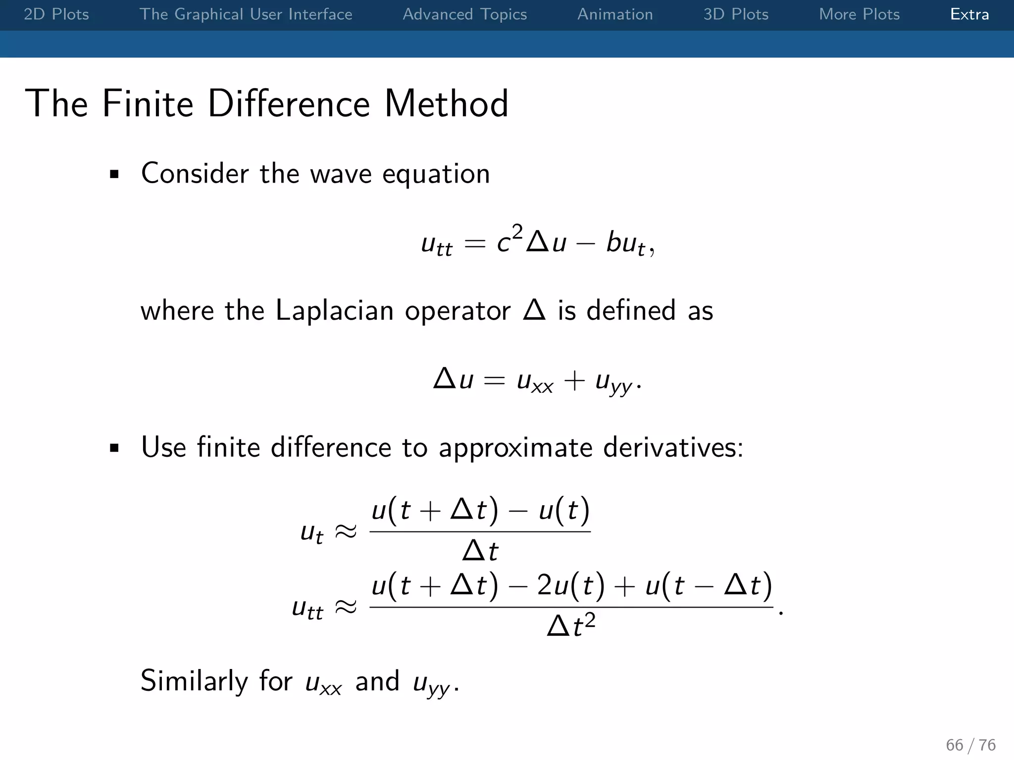
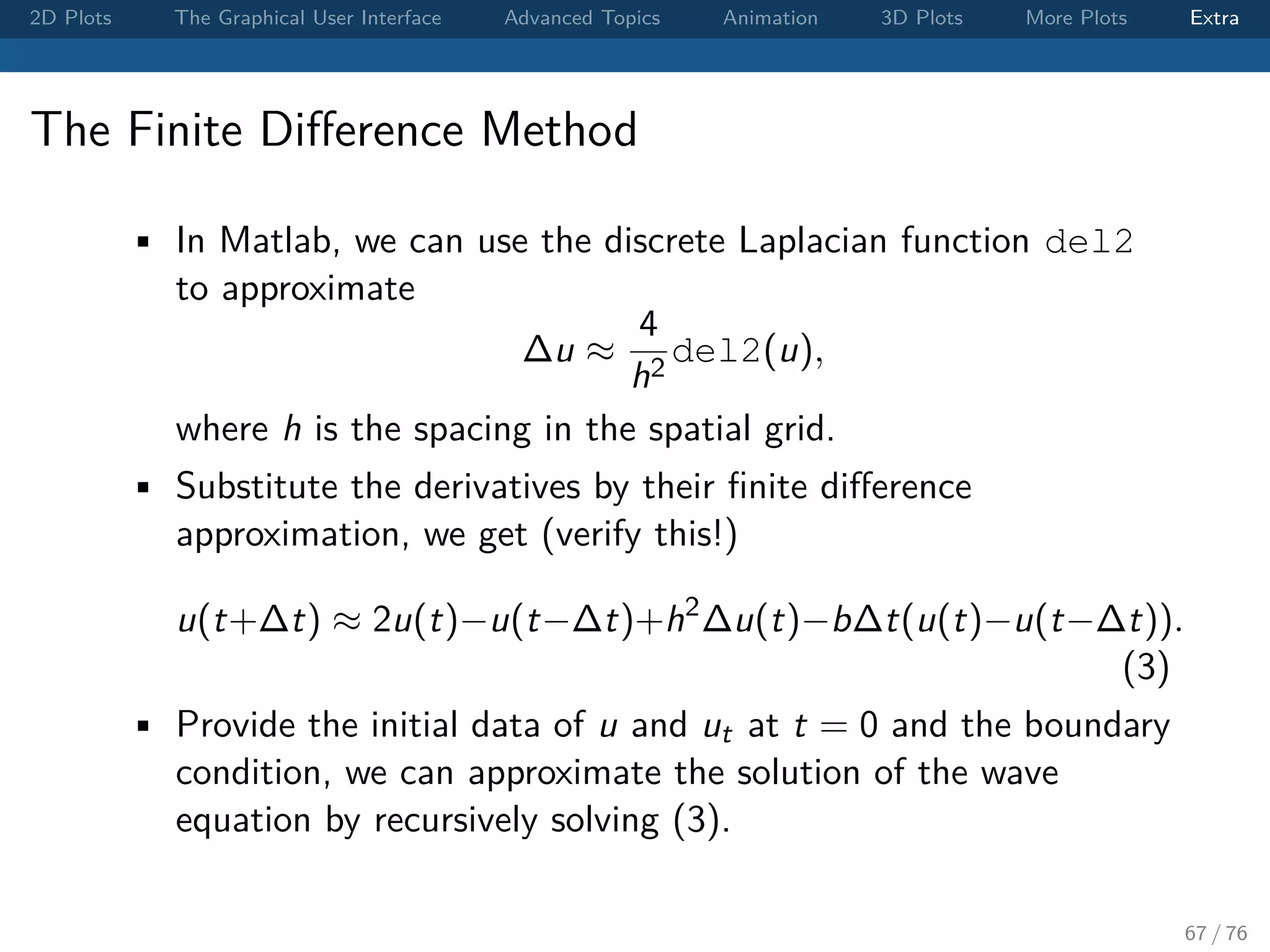
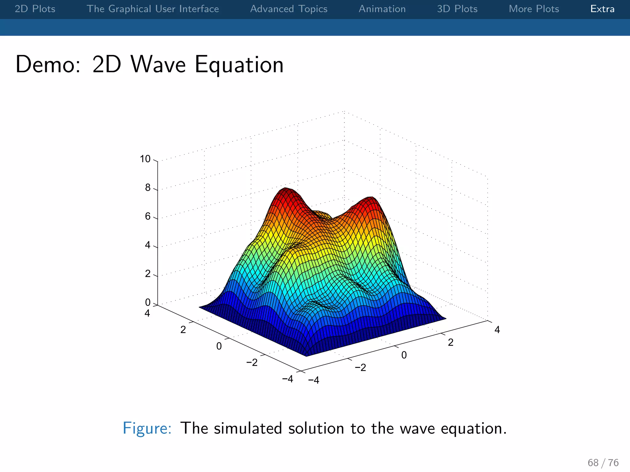
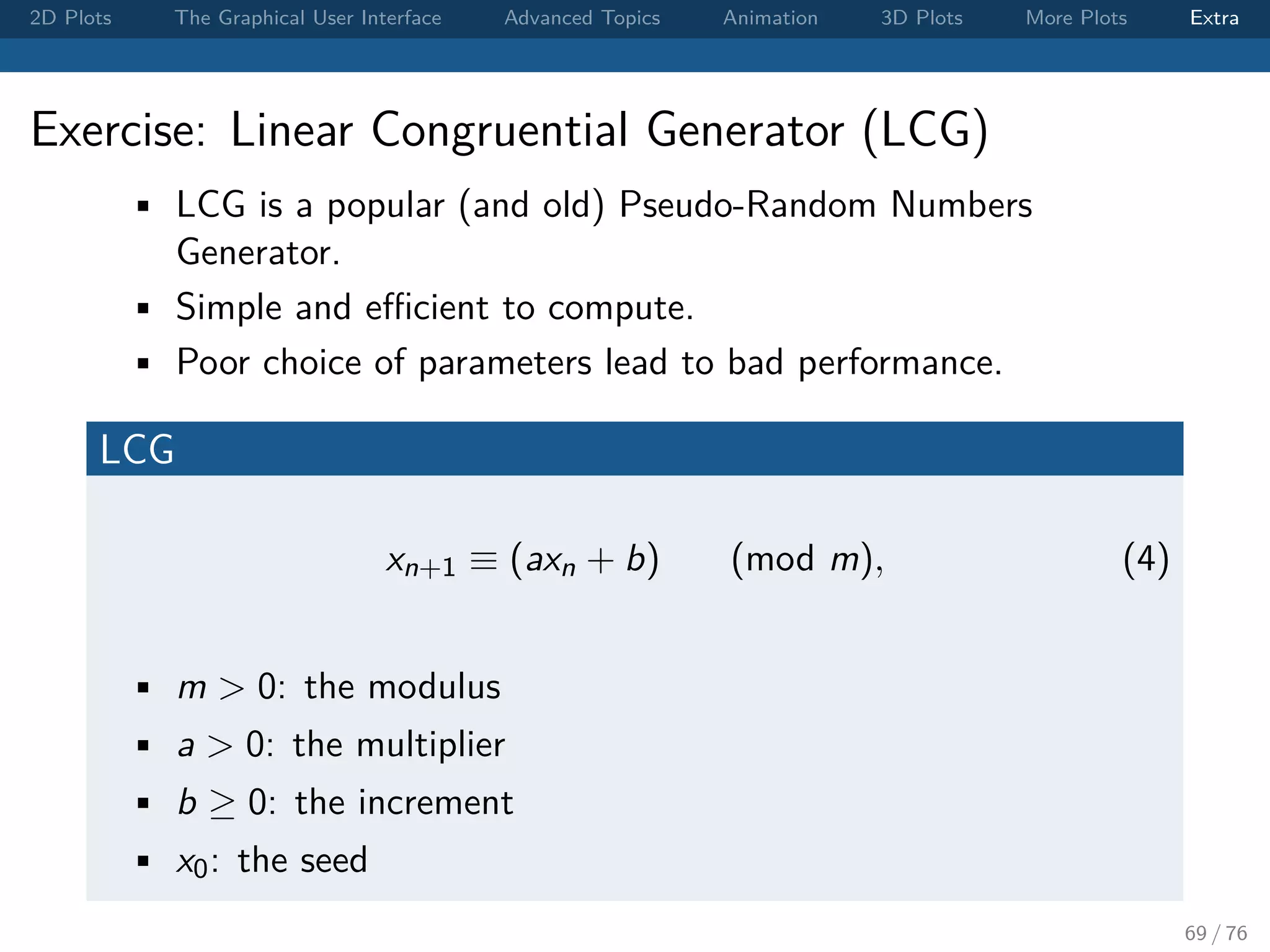
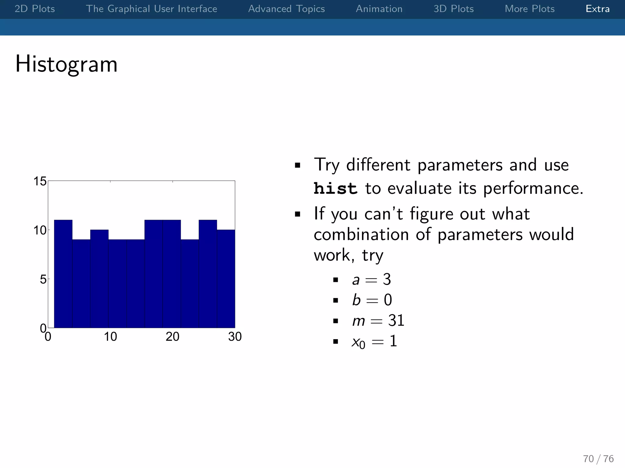
Download as PDF, PPTX
![2D Plots The Graphical User Interface Advanced Topics Animation 3D Plots More Plots Extra Changing the Axes Limits Syntax • Set the limits of each axis axis([xmin xmax ymin ymax]); • If you want to adjust only x-axis or y-axis, xlim([xmin xmax]); ylim([ymin ymax]); 11 / 76](https://image.slidesharecdn.com/matlabplottutorial2013summer-150903200119-lva1-app6891/75/Matlab-Graphics-Tutorial-11-2048.jpg)
![2D Plots The Graphical User Interface Advanced Topics Animation 3D Plots More Plots Extra Exercise: Plot Matrix Data Let Y = [ y1; y2; y3 ]; • What is the dimension of Y? • Try plot(t,Y) and plot(Y). Can you anticipate the outputs? 15 / 76](https://image.slidesharecdn.com/matlabplottutorial2013summer-150903200119-lva1-app6891/75/Matlab-Graphics-Tutorial-15-2048.jpg)
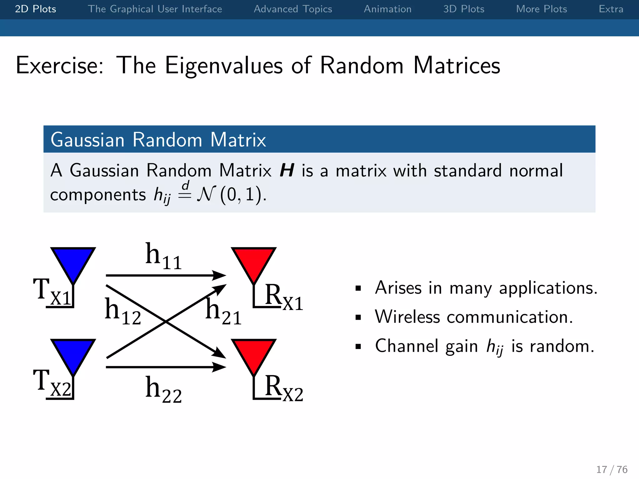
![2D Plots The Graphical User Interface Advanced Topics Animation 3D Plots More Plots Extra Exercise: The Eigenvalues of Random Matrices Visualizing the distribution of the eigenvalues of random matrices. • Generate H = randn(n,n). • [V,D] = eig(H). • Plot its eigenvalues as dots on the complex plane. • Increase n form 10 to 1, 000. Can you tell what’s the pattern of the eigenvalues? 18 / 76](https://image.slidesharecdn.com/matlabplottutorial2013summer-150903200119-lva1-app6891/75/Matlab-Graphics-Tutorial-18-2048.jpg)


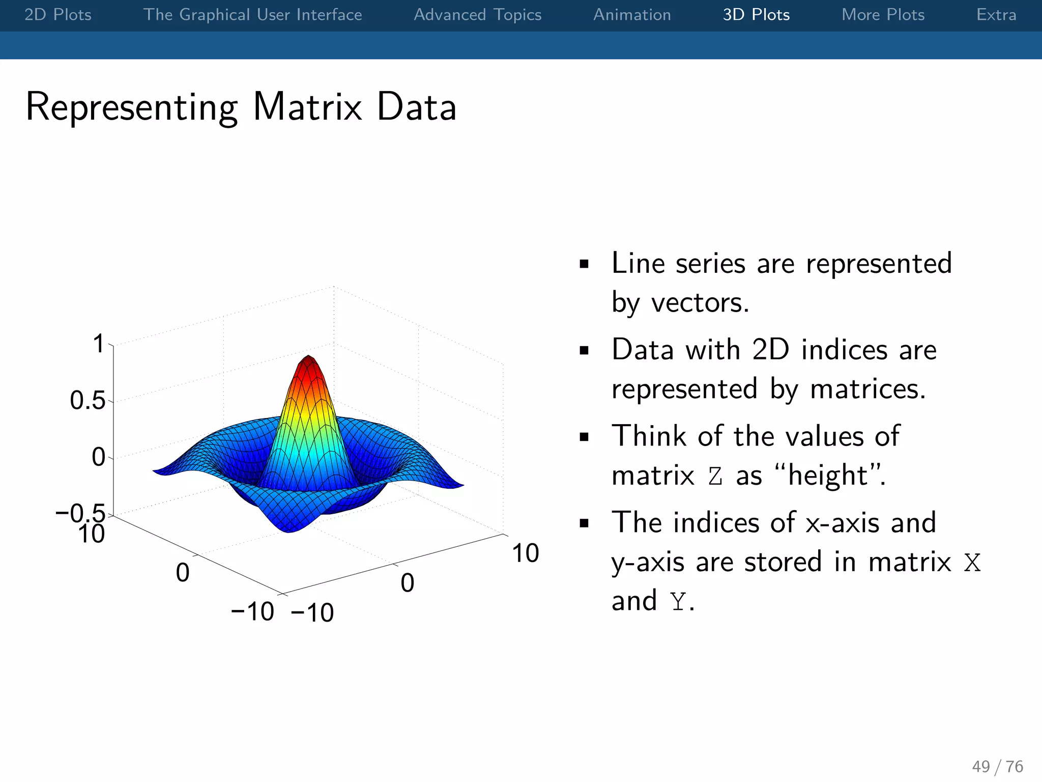
![2D Plots The Graphical User Interface Advanced Topics Animation 3D Plots More Plots Extra Mesh Grid and Surface Plot To visualize a function f (x, y) on (x, y) ∈ [a, b] × [c, d], • First we need to create a rectangular grid. • Matlab provides a useful function to create such a grid: [X,Y] = meshgrid(x,y); where x and y are the sampling points on both axis. • Then we can use surf(X,Y,f(X,Y)); to produce a surface plot. 50 / 76](https://image.slidesharecdn.com/matlabplottutorial2013summer-150903200119-lva1-app6891/75/Matlab-Graphics-Tutorial-50-2048.jpg)
![2D Plots The Graphical User Interface Advanced Topics Animation 3D Plots More Plots Extra Exercise: The 3D Sinc Function 3D Sinc Function sinc(r) := sin(r) r , where r2 = x2 + y2. • Visualize the 3D sinc function on (x, y) ∈ [−8, 8] × [−8, 8]. • One way to avoid the divided-by-zero error is to use sin(r)./(r+esp) instead of sin(r)./r. • esp is the smallest representable floating point number in Matlab. 51 / 76](https://image.slidesharecdn.com/matlabplottutorial2013summer-150903200119-lva1-app6891/75/Matlab-Graphics-Tutorial-51-2048.jpg)
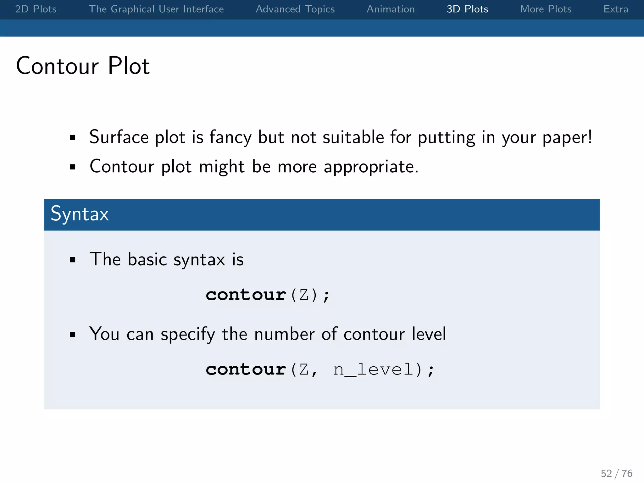
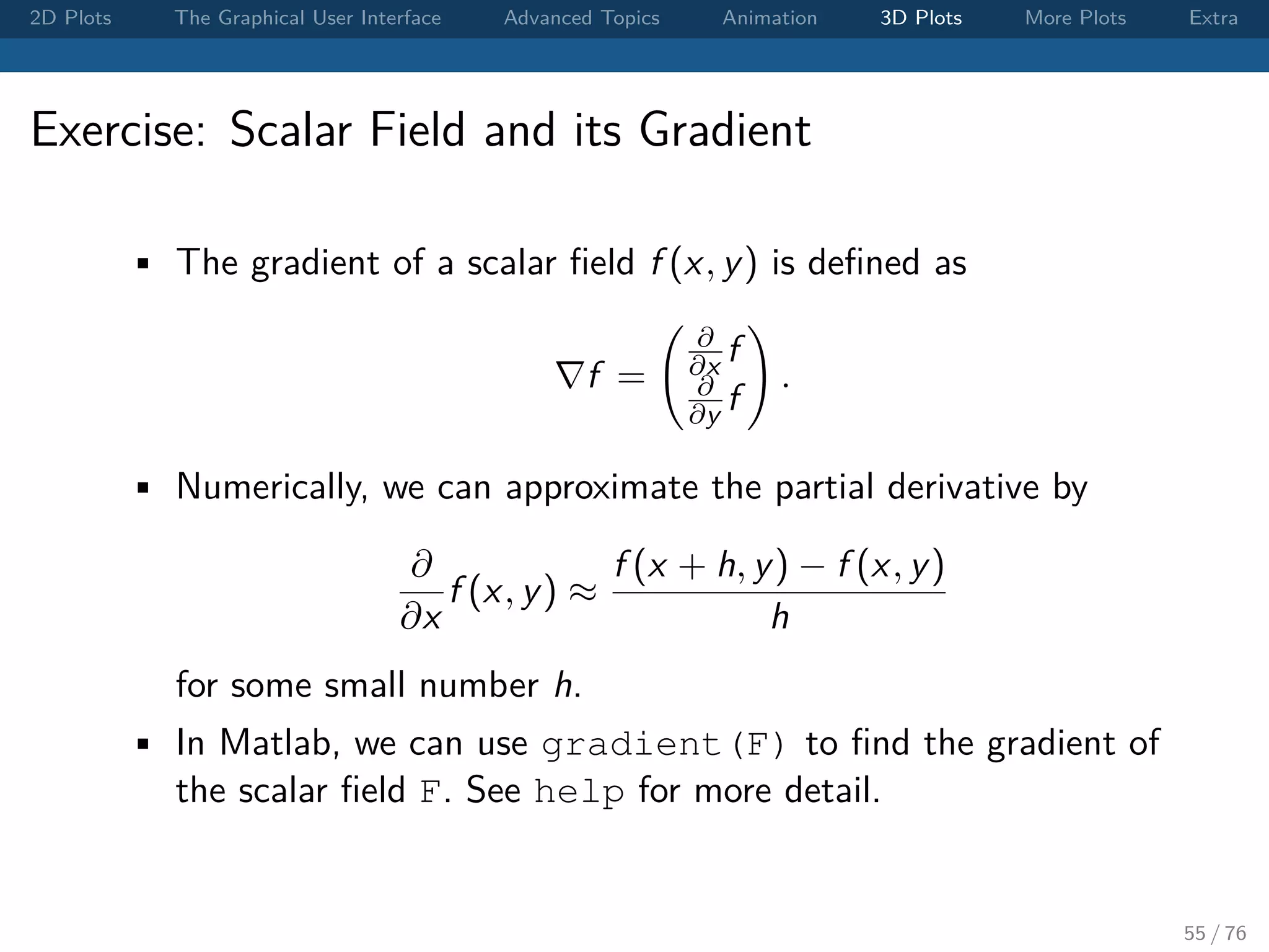
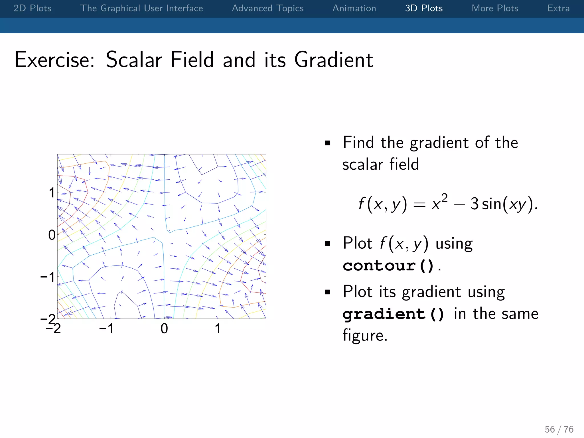
![2D Plots The Graphical User Interface Advanced Topics Animation 3D Plots More Plots Extra Exercise: Scalar Field Let f (x, y) = x2 − 3 sin(xy). Use contour plot to visualize f (x, y) on [−2, 2] × [−2, 2]. 53 / 76](https://image.slidesharecdn.com/matlabplottutorial2013summer-150903200119-lva1-app6891/75/Matlab-Graphics-Tutorial-53-2048.jpg)

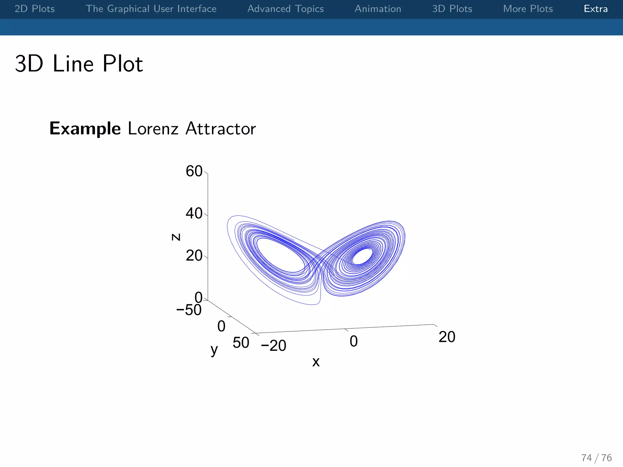

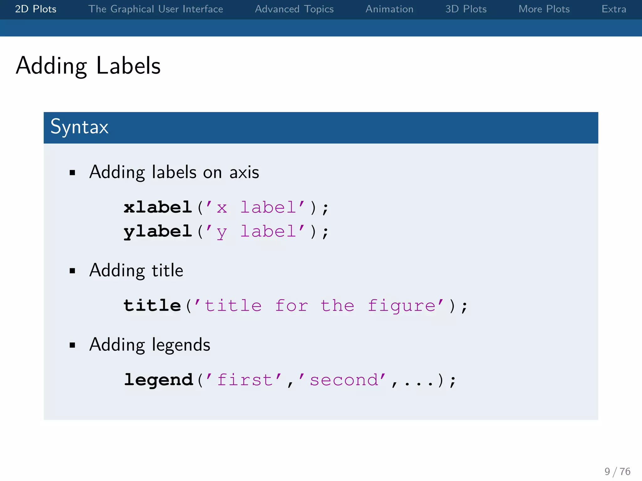
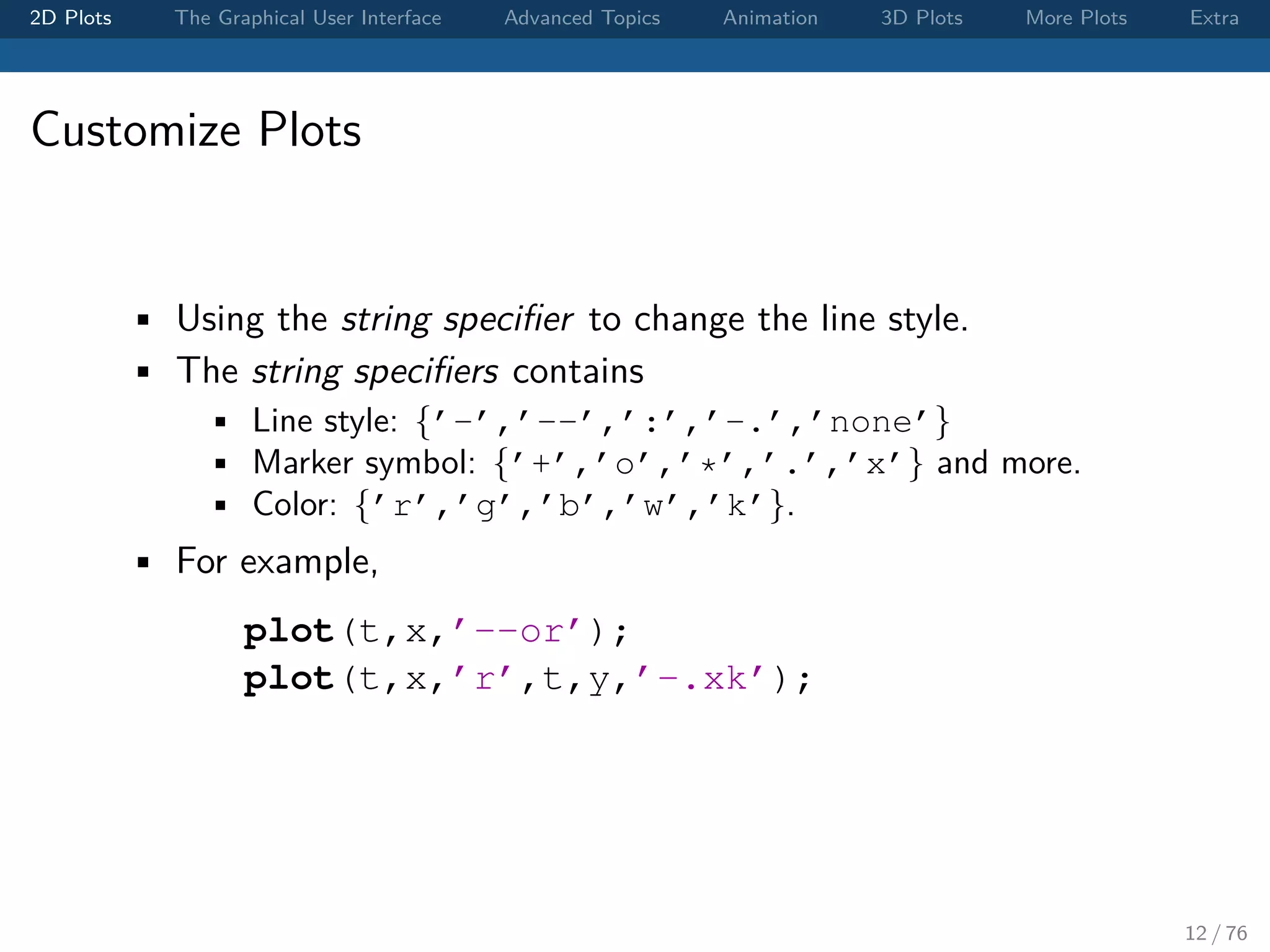
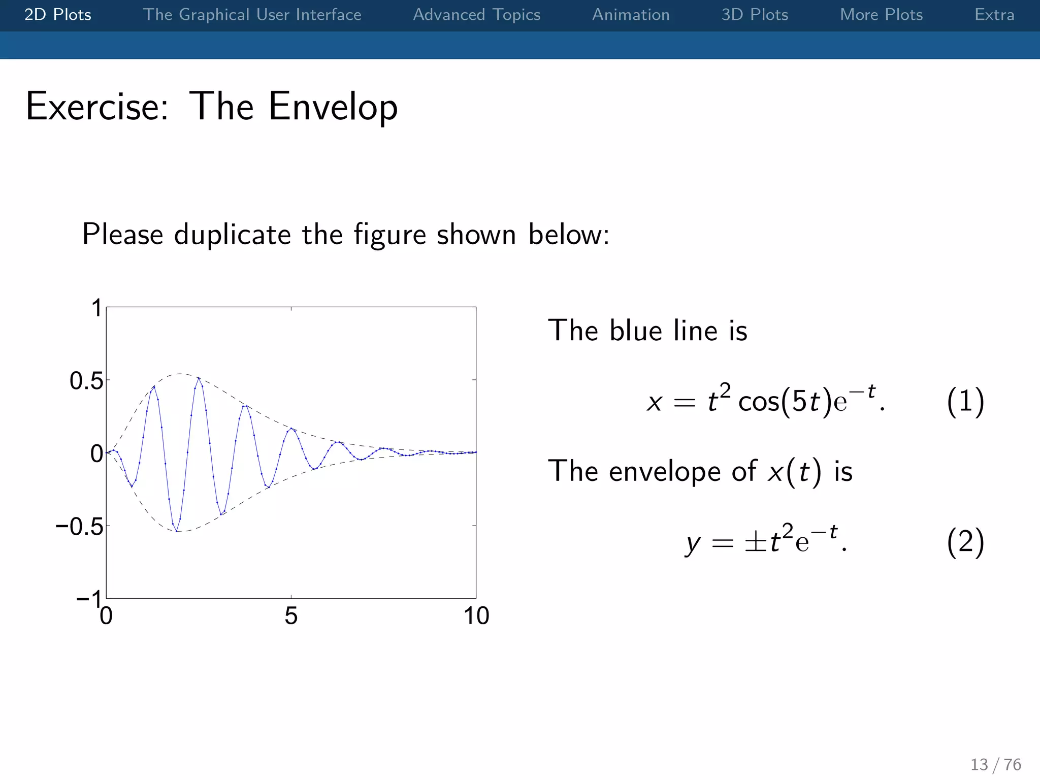
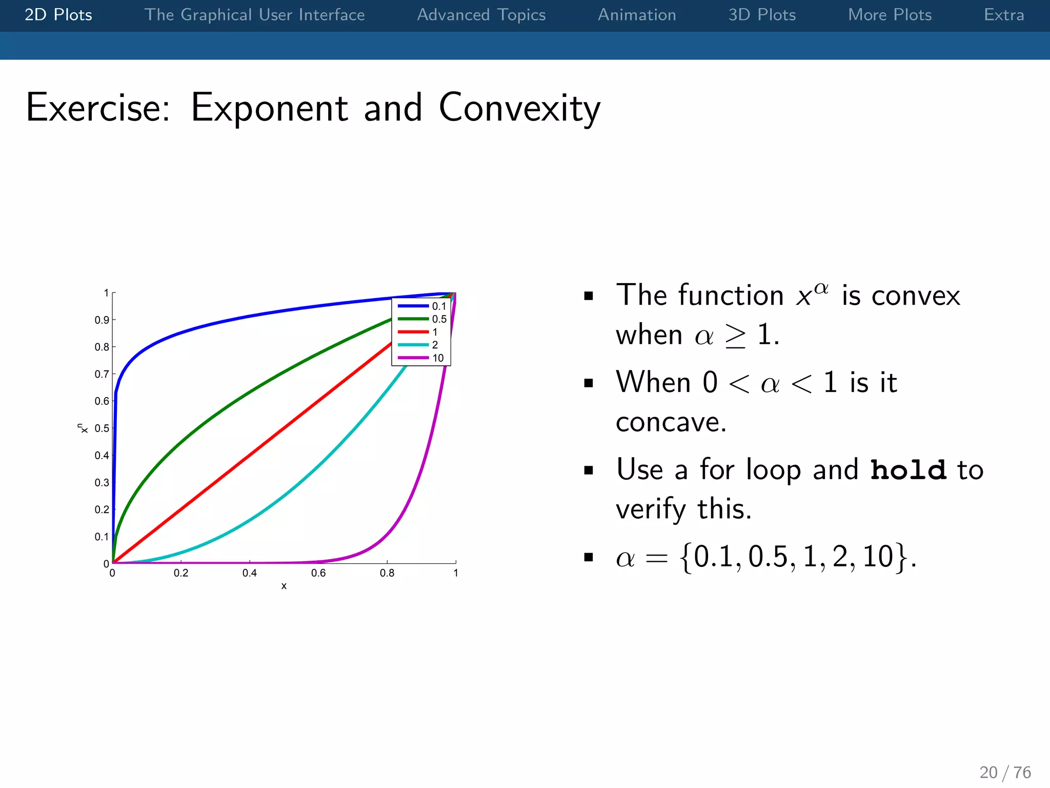
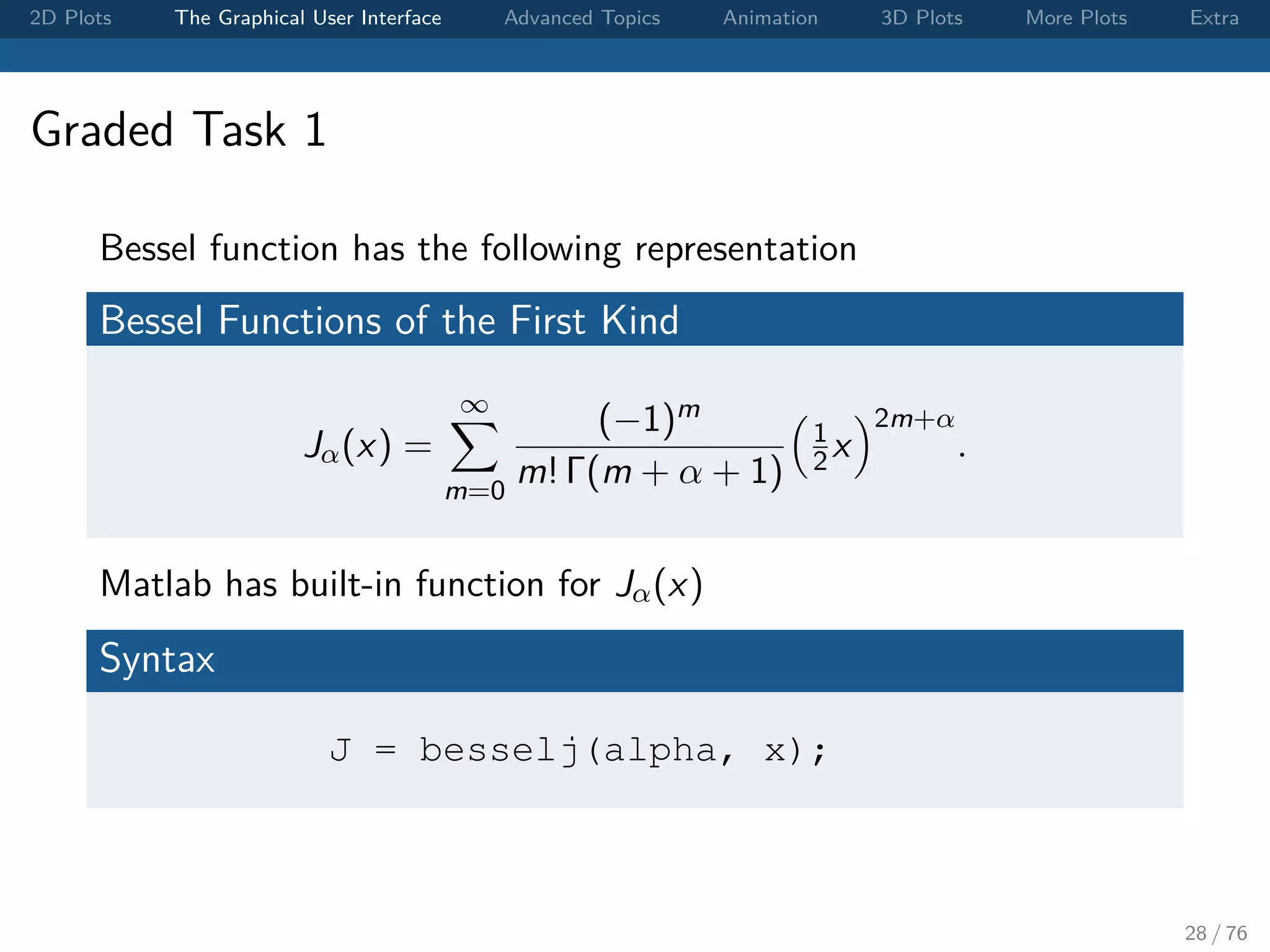
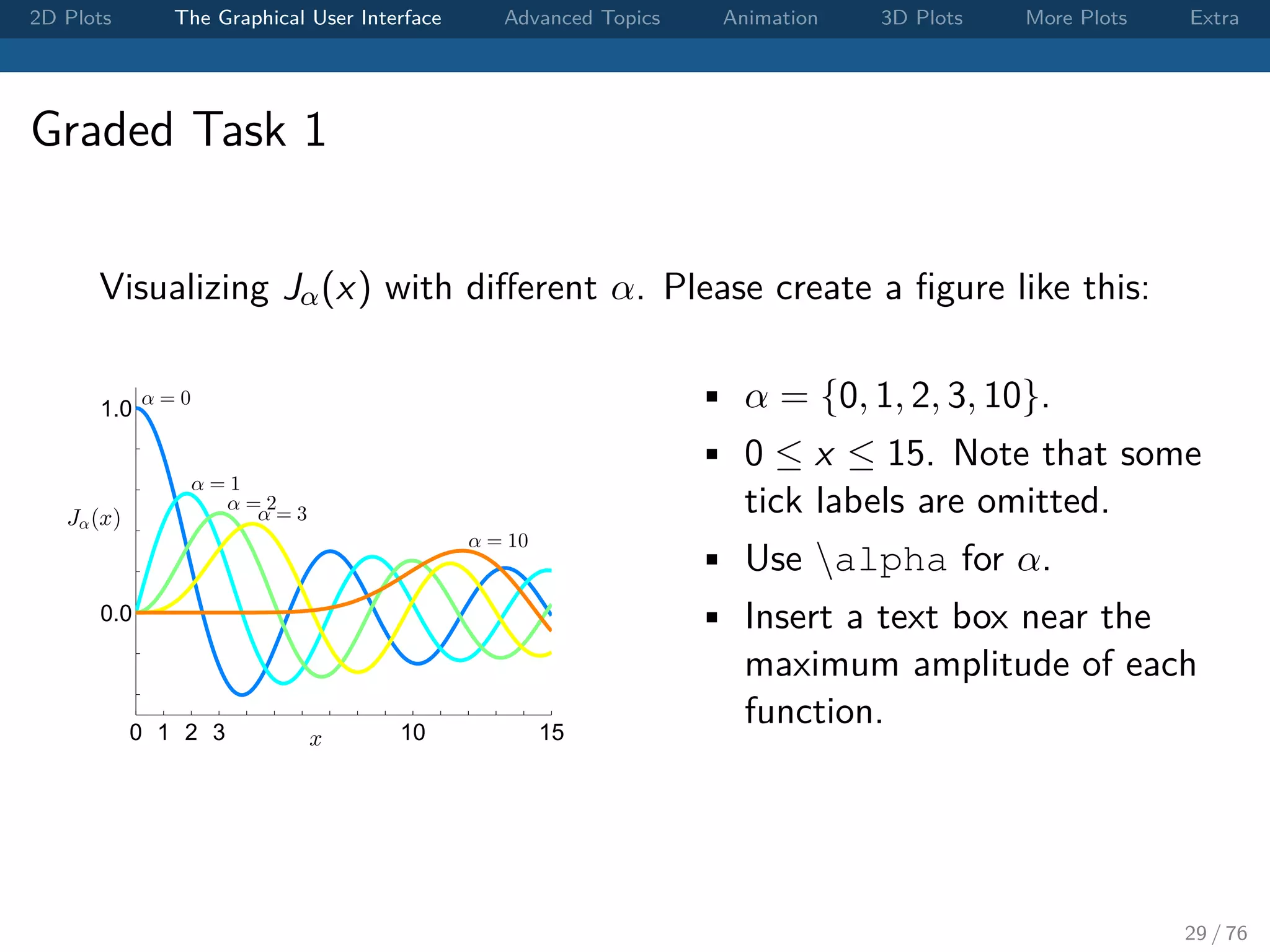
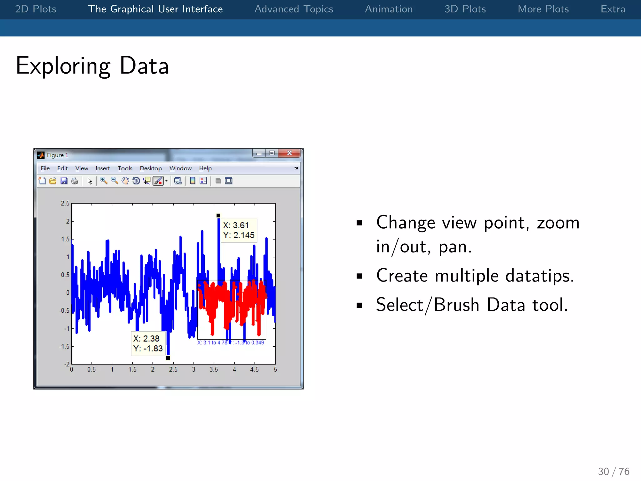
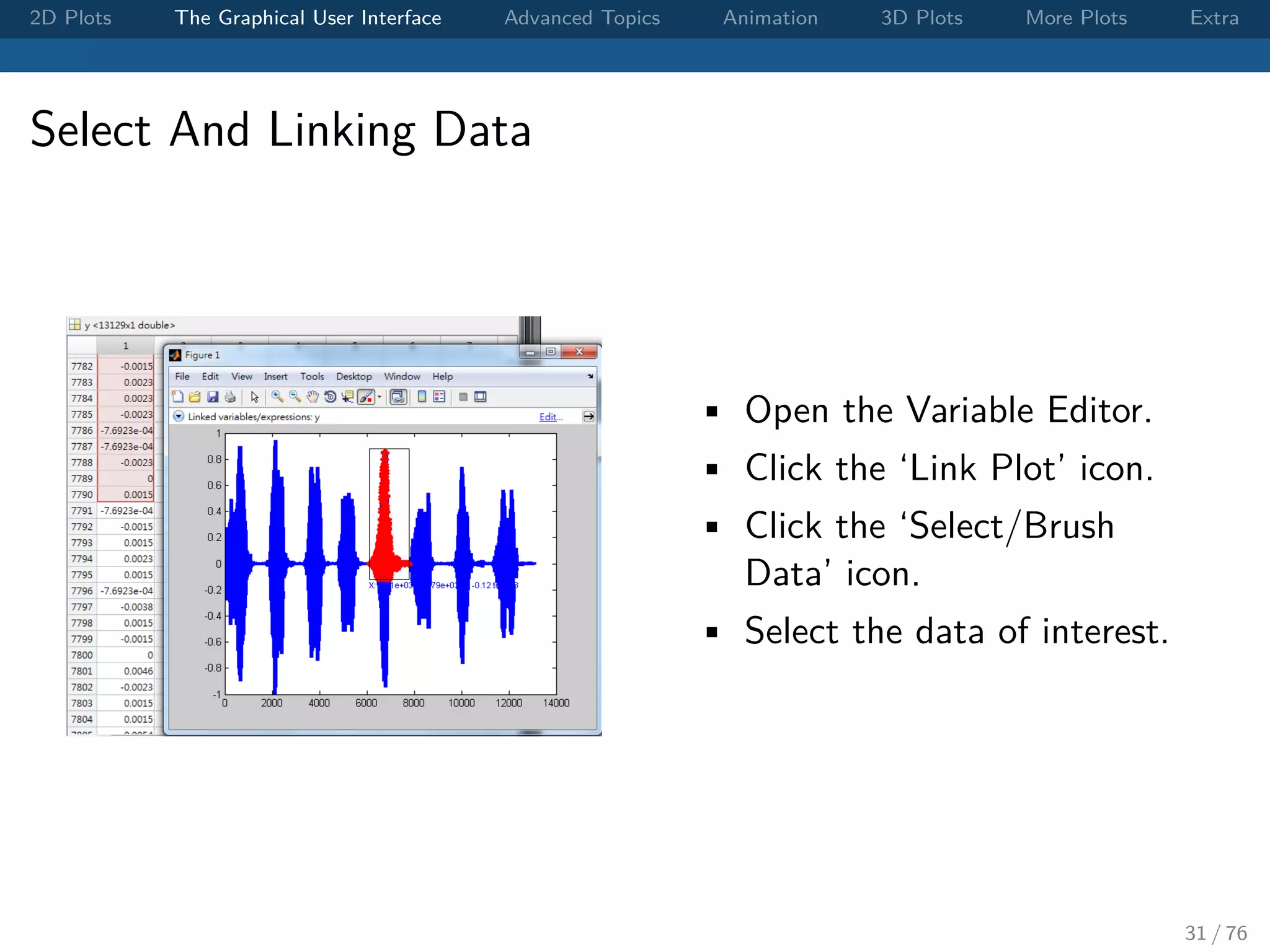
The document outlines various MATLAB plotting techniques, focusing on 2D and 3D plots, graphical user interface functions, and advanced topics such as animation. It provides syntax examples for creating figures, customizing plots, and includes exercises for visualizing mathematical functions. Additionally, it discusses batch processing and handling graphical objects within MATLAB.