This document provides an introduction and overview of MATLAB. It discusses what MATLAB is, its main features and interfaces. Some key points covered include: - MATLAB is a computing environment for doing matrix manipulations, calculations and data analysis. It has specialized toolboxes for tasks like signal processing and system analysis. - The main interfaces are the command window, workspace, command history and editor window. Commands can be executed directly, through script files or custom functions. - MATLAB handles matrices and vectors natively and has extensive math and graphics functions. Basic operations include matrix/vector creation, arithmetic, plotting and flow control structures. - Help is available through the help menu, demos and documentation. Common functions covered
Introduction to MATLAB by Mr. M. Ravi. Overview of MATLAB as a high-level language with toolboxes, focusing on essential features like command line and data handling.
MATLAB excels in computational tasks, handling matrices and data analysis. Its ability to plot, compute through functions, and visualize data through various methods is highlighted.
Description of MATLAB's user interface components, including Command Window, Workspace, Command History, and Editor, essential for tasks and command execution.
Fundamentals of vectors and matrices in MATLAB, including definition methods, manipulation, and arithmetic operations, showcasing how to create and handle matrices.
Introduction to MATLAB's help functionality, including use of built-in demos and accessing documentation for various functions to aid learning and usage.
Essentials of programming in MATLAB, including comments, defining functions, and control structures such as loops and conditions crucial for scripting.
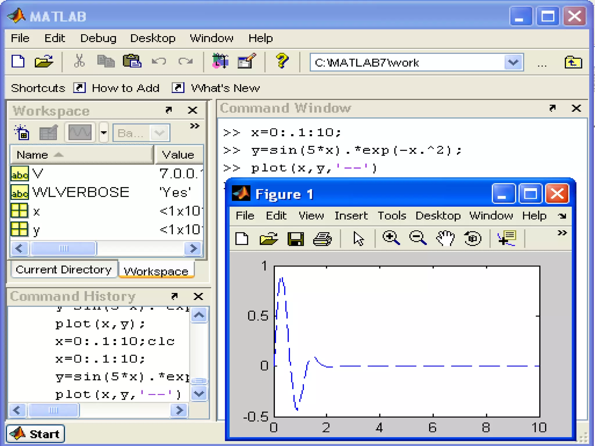
Techniques for generating and plotting basic signals using MATLAB functions. Covers syntax for creating various types of plots and their customization.
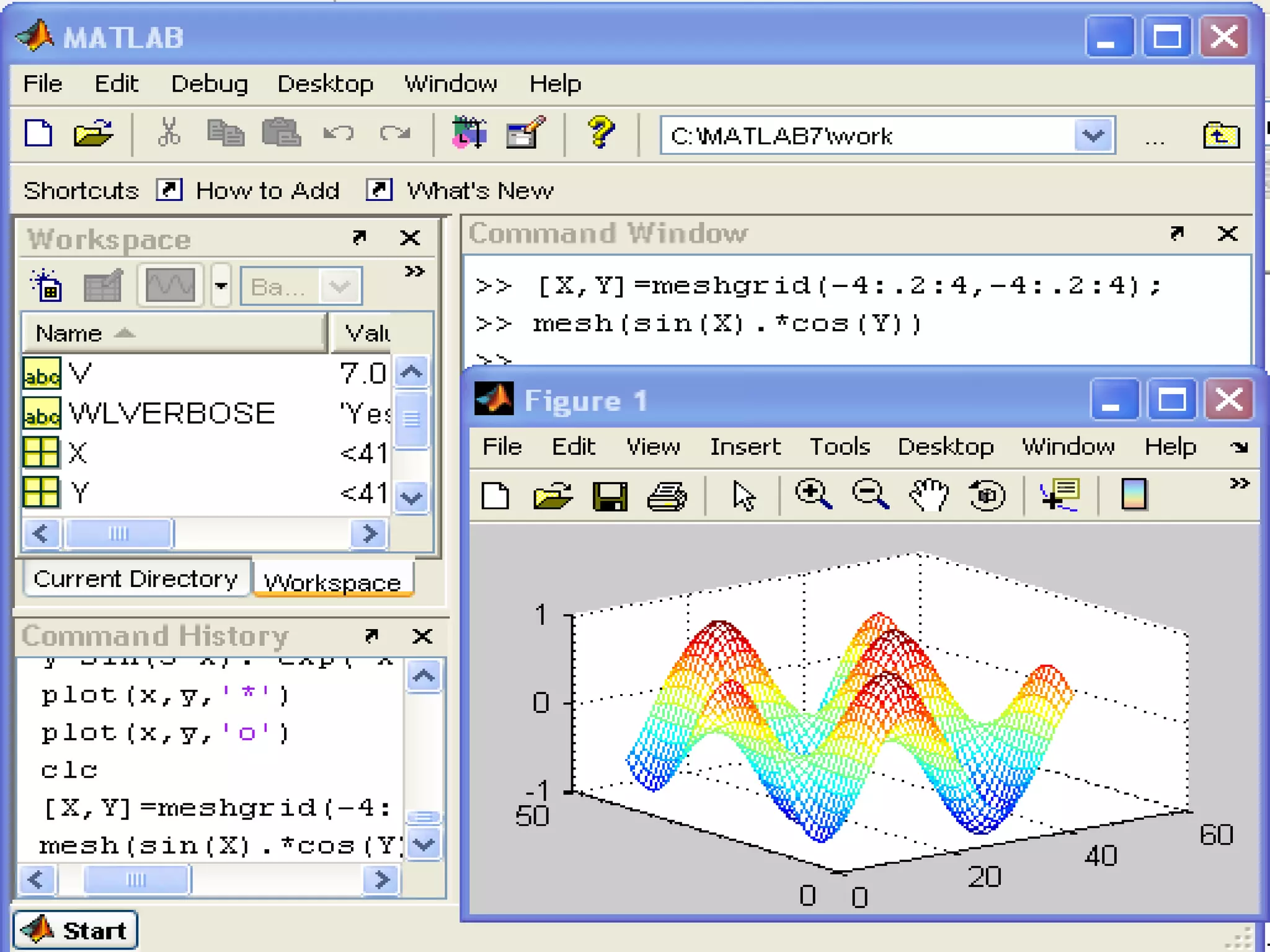
Advanced plotting techniques, including continuous and discrete representation, use of random numbers for statistical visualization, and MATLAB commands for managing workspace.
Wrap-up of the presentation, thanking participants, and indicating the end of the session.
What is Matlab? •Matlab is basically a high level language which has many specialized toolboxes for making things easier for us Assembly High Level Languages such as C, Pascal etc. Matlab
3.
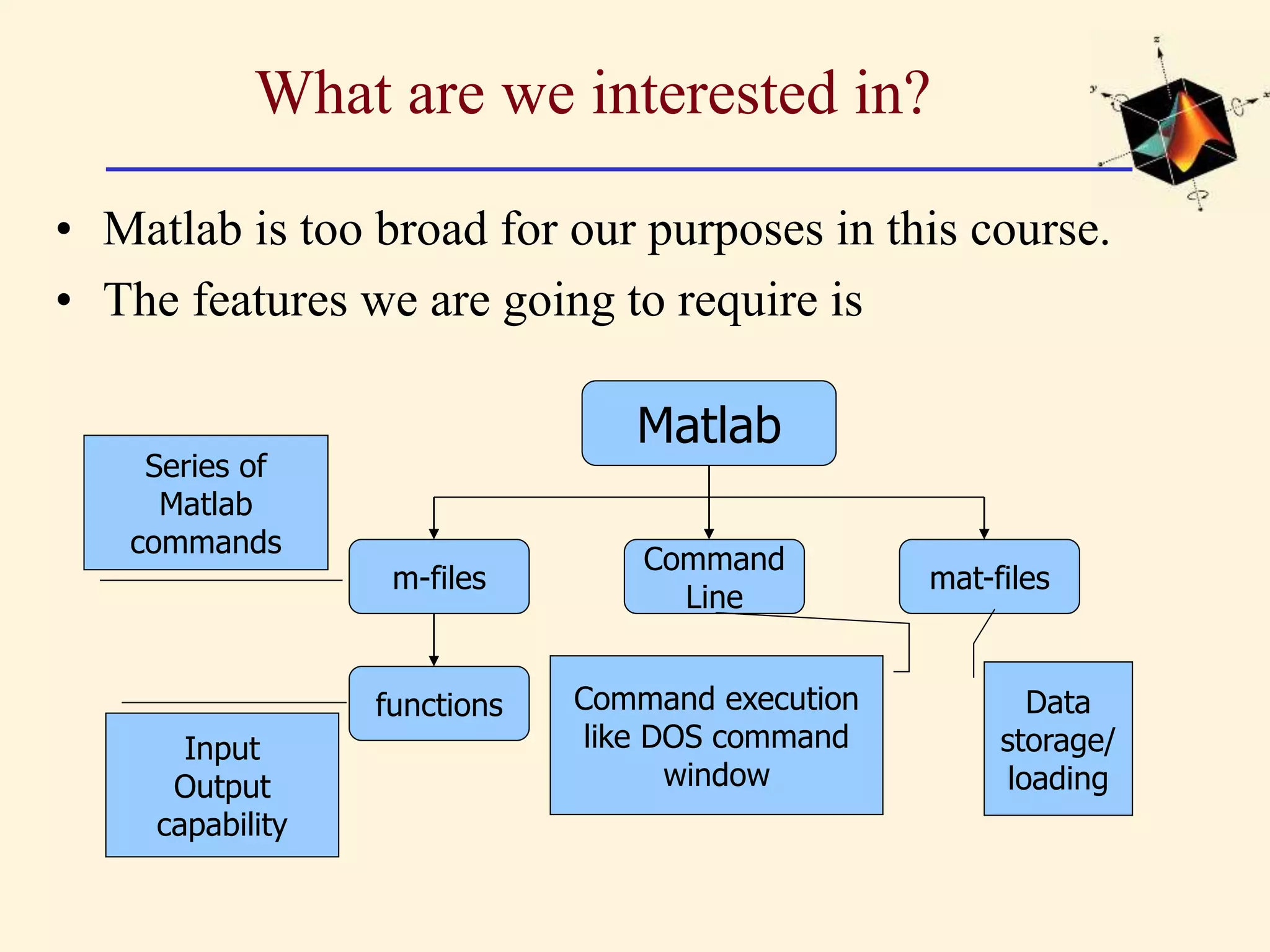
What are weinterested in? • Matlab is too broad for our purposes in this course. • The features we are going to require is Matlab Command Line m-files functions mat-files Command execution like DOS command window Series of Matlab commands Input Output capability Data storage/ loading
Introduction • MATLAB (shortfor MATrix LABoratory) is a powerful computing environment that handles anything from simple arithmetic to advanced data analysis. • At its core is the matrix as its basic data type. • Combined with extensive maths and graphics functions, complicated calculations can be carried out by specifying only a few simple instructions. • MATLAB can be used to do anything your scientific calculator can do, and more. • The installations in the computer labs include tool boxes that include functions for electrical engineering related tasks, such as signal processing and system analysis.
6.
Introduction. . .. • You can plot your data in a multitude of visualizations as well. • Computations can be carried out in one of three ways: 1. Directly from the command line, 2. by writing a script that carries out predefined instructions, or 3. by writing your own functions.
7.
Introduction . .. • Writing your own functions is much like programming in other languages, except that you have the full resources of MATLAB’s functions at your disposal, making for very compact code. The MATLAB-6 and above environment has several windows at your disposal. • Command Window: The main window is the command window, where you will type all your commands, for small programs.
8.
Desktop Tools • CommandWindow – type commands • Workspace – view program variables – Clear/clear all is used to clear the workspace window – double click on a variable to see it in the Array Editor • Command History – view past commands – save a whole session using diary • Editor Window To write a program • Current Directory Window
10.
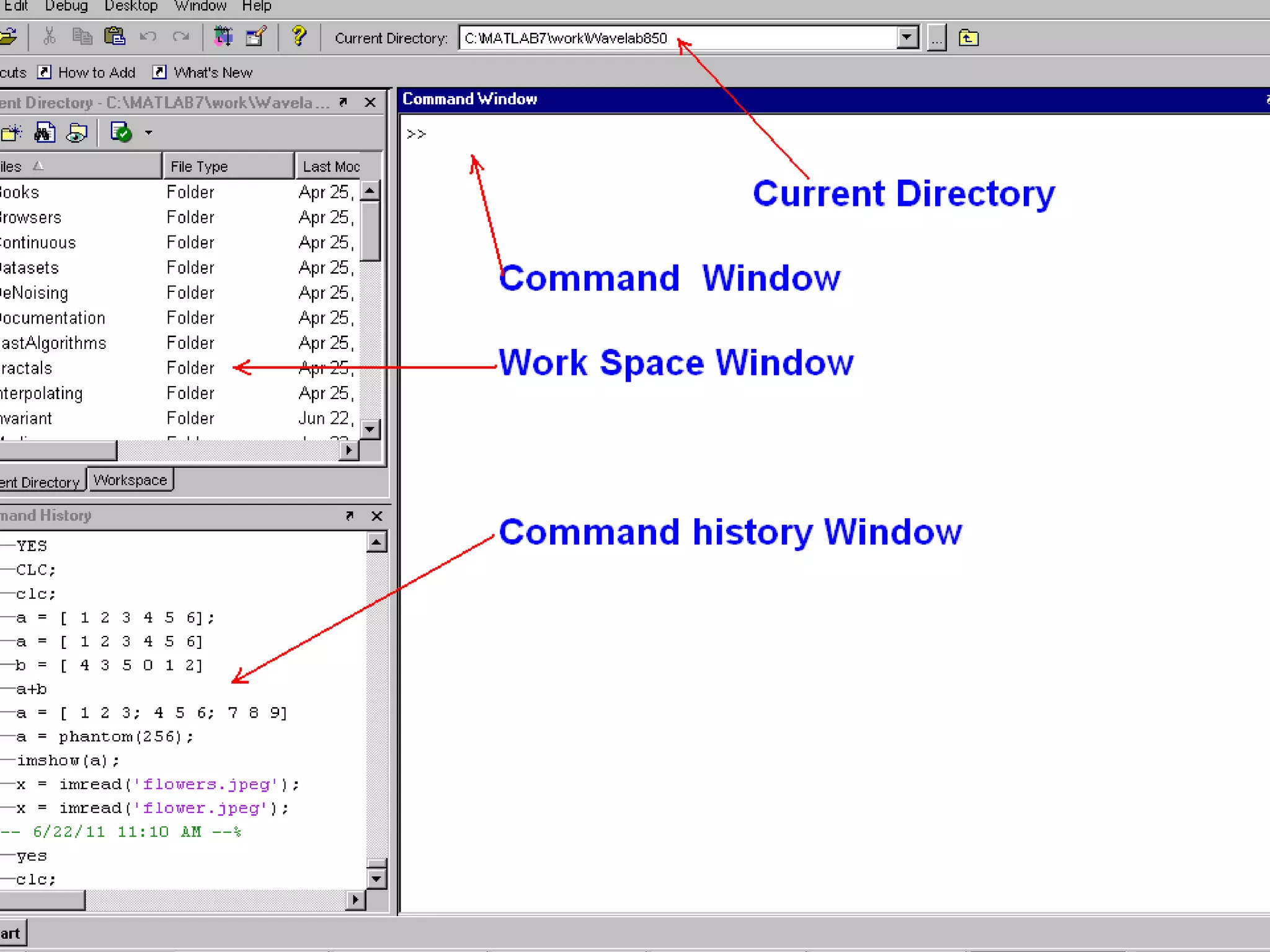
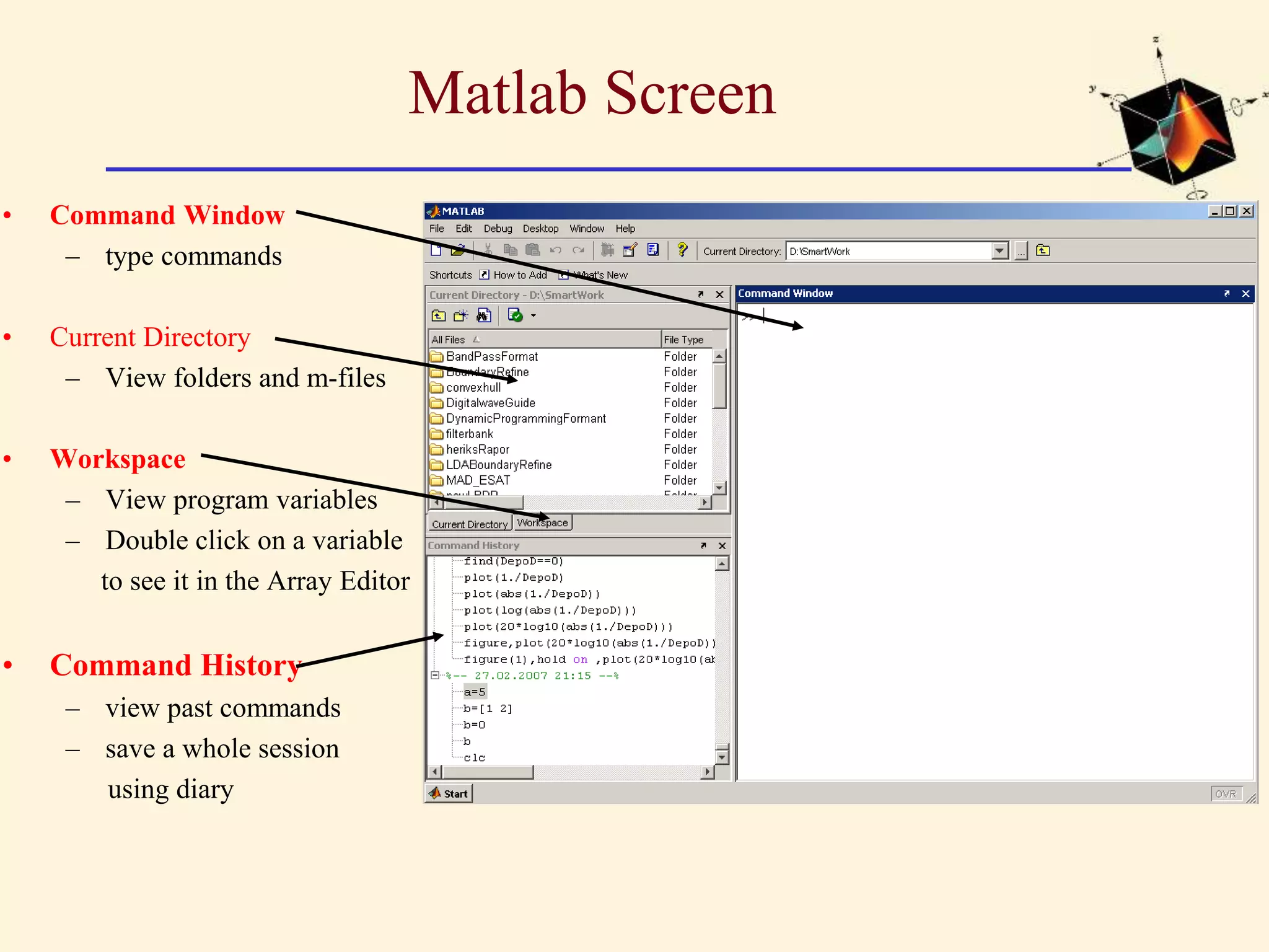
Matlab Screen • CommandWindow – type commands • Current Directory – View folders and m-files • Workspace – View program variables – Double click on a variable to see it in the Array Editor • Command History – view past commands – save a whole session using diary
11.
Command History * Acommand history, which contains a list of all the commands that you have typed in the command window. * This makes it easy to cut and paste earlier lengthy commands, saving you the effort of typing it over again. * This window can also display the contents of the current directory.
12.
Workspace • The thirdwindow displays one of two things: * The launch pad from which you can browse the installed toolboxes and launch various tools as well as view demonstrations, and * The workspace, which lists all the variables that are currently in memory as well as their sizes.
Definition of Vectors& Matrices • MATLAB is based on matrix and vector algebra; even scalars are treated as 1x1 matrices. Therefore, vector and matrix operations are as simple as common calculator operations. • Vectors can be defined in two ways. * The first method is used for arbitrary elements: v = [1 3 5 7]; creates a 1x4 vector with elements 1, 3, 5 and 7. * Note that commas could have been used in place of spaces to separate the elements. that is v=[1,3,5,7]; • Additional elements can be added to the vector: v(5) = 8; yields the vector v = [1 3 5 7 8].
16.
• Previously definedvectors can be used to define a new vector. For example, with ‘v’ defined above a = [9 10]; b = [v a]; creates the vector b = [1 3 5 7 8 9 10].
17.
Second Method • Thesecond method is used for creating vectors with equally spaced elements: t = 0: 0.1:10; creates a 1x101 vector with the elements 0, .1, .2, .3,...,10. Note that the middle number defines the increment. • If only two numbers are given, then the increment is set to a default of 1: For ex. k = 0:10; creates a 1x11 vector with the elements 0, 1, 2, ..., 10.
18.
* Matrices aredefined by entering the elements row by row: M = [1 2 4; 3 6 8; 2 6 5]; creates the matrix * Transpose of M is denoted by M’, and displays as *The inverse of M is M-1 denoted in Matlab as M^-1and displays as * M(2,3) displays the element of second row and third column
19.
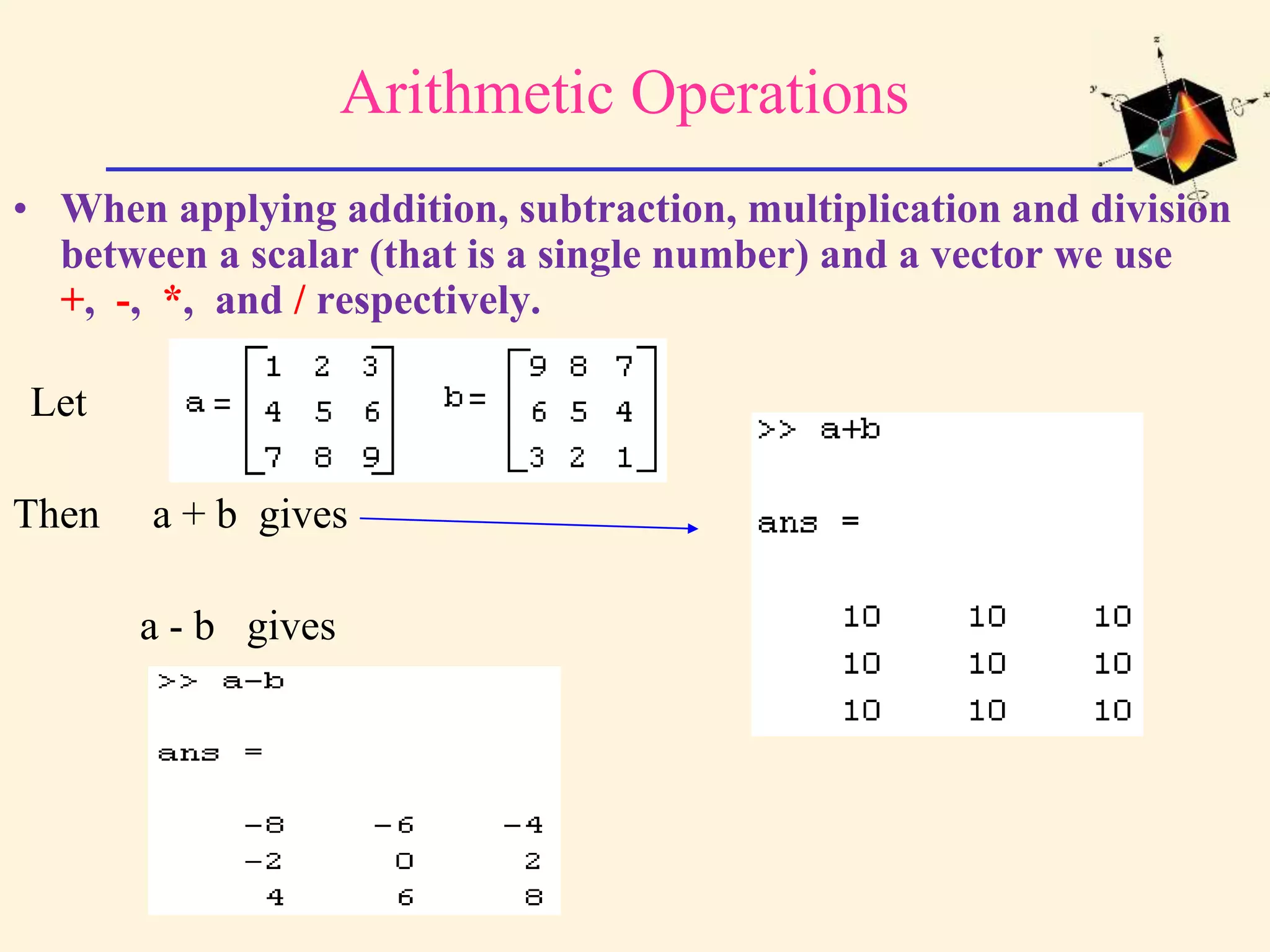
Arithmetic Operations • Whenapplying addition, subtraction, multiplication and division between a scalar (that is a single number) and a vector we use +, -, *, and / respectively. Let Then a + b gives a - b gives
20.
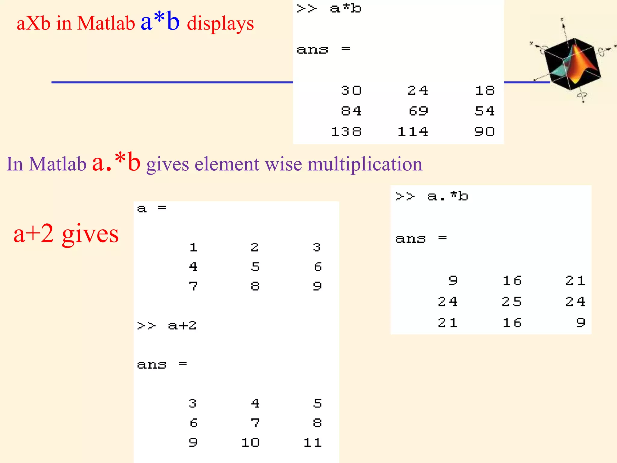
aXb in Matlaba*b displays In Matlab a.*b gives element wise multiplication a+2 gives
21.
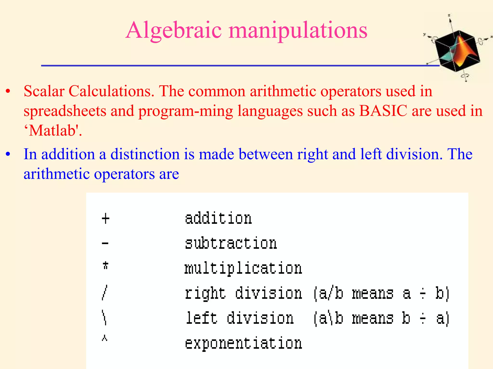
Algebraic manipulations • ScalarCalculations. The common arithmetic operators used in spreadsheets and program-ming languages such as BASIC are used in ‘Matlab'. • In addition a distinction is made between right and left division. The arithmetic operators are
22.
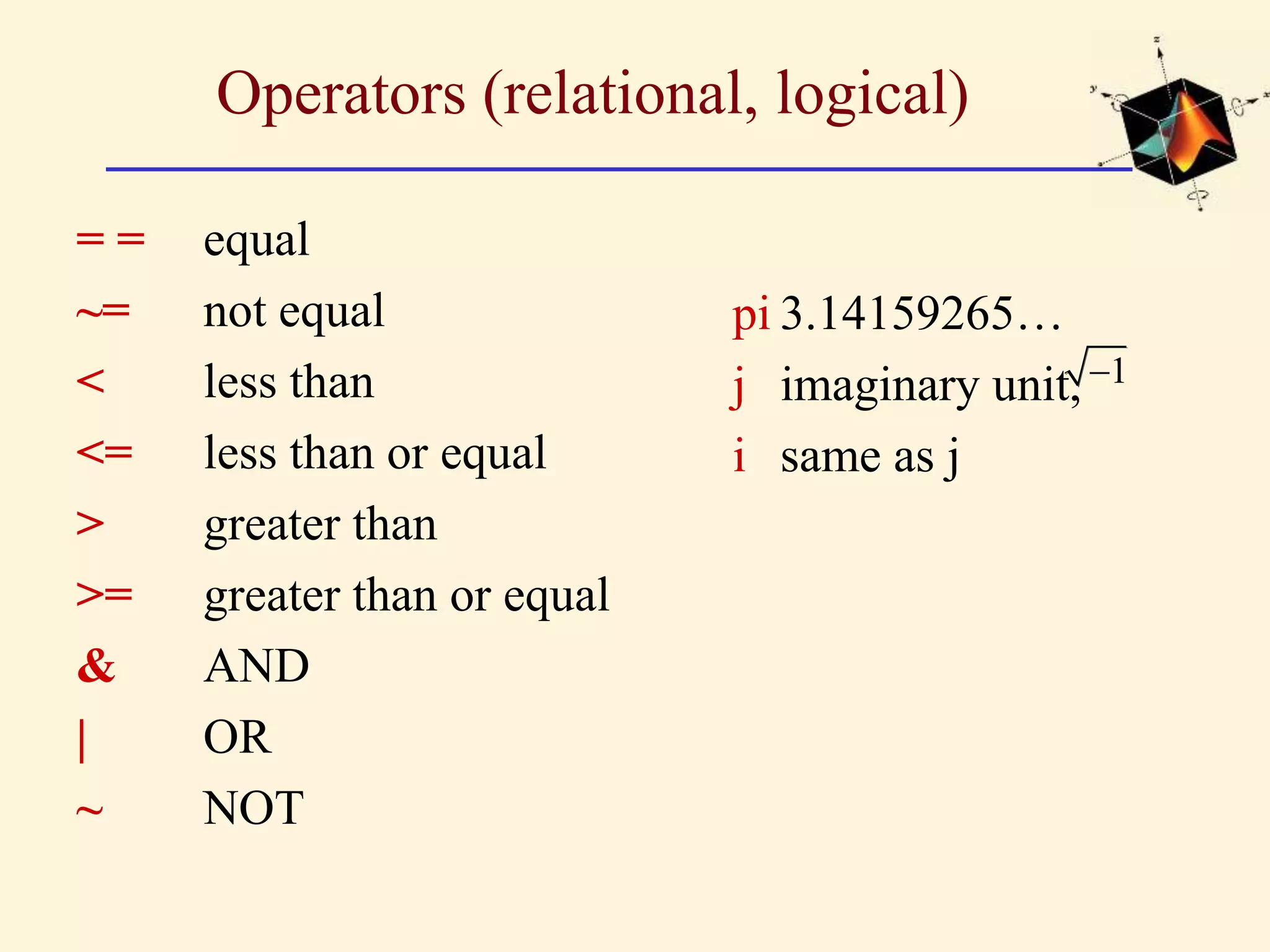
Operators (relational, logical) == equal ~= not equal < less than <= less than or equal > greater than >= greater than or equal & AND | OR ~ NOT 1 pi 3.14159265… j imaginary unit, i same as j
23.
Special Matrices • nullmatrix: M = [ ]; • nxm matrix of zeros: M = zeros(n,m); nxm matrix of ones: M = ones(n,m); nxn identity matrix: M = eye(n);
24.
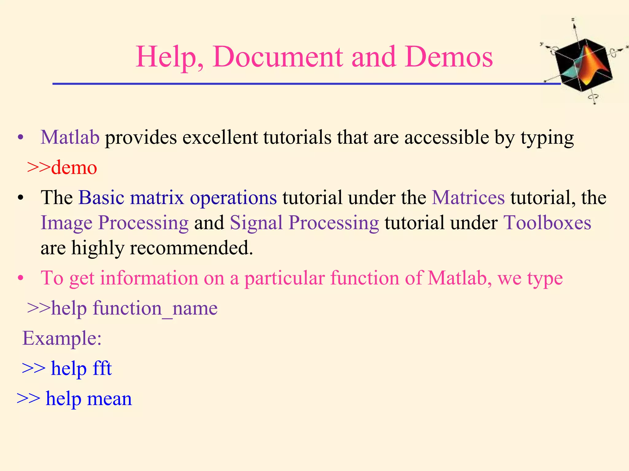
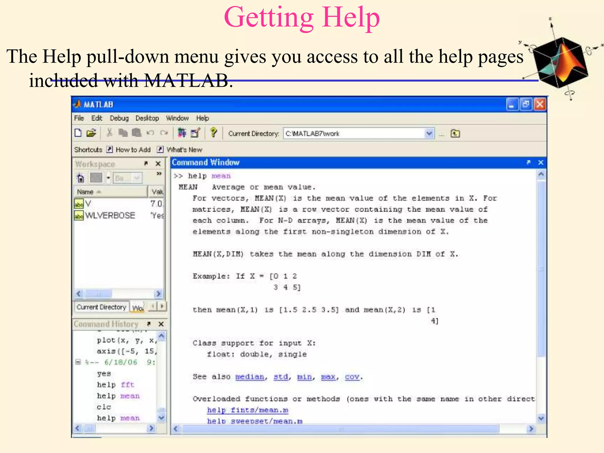
Help, Document andDemos • Matlab provides excellent tutorials that are accessible by typing >>demo • The Basic matrix operations tutorial under the Matrices tutorial, the Image Processing and Signal Processing tutorial under Toolboxes are highly recommended. • To get information on a particular function of Matlab, we type >>help function_name Example: >> help fft >> help mean
25.
Getting Help The Helppull-down menu gives you access to all the help pages included with MATLAB.
26.
• Comments inMatlab must be proceeded by % % This is a comment in Matlab. • To define a function in Matlab, we first create a function with the name of the function. *We then define the function in the file. *For example, the Matlab documentation recommends stat.m written as: function [mean,stdev] = stat(x) % This comment is printed out with help stat n = length(x); % assumes that x is a vector. mean = sum(x) / n; % sum adds up all elements. stdev = sqrt(sum((x - mean).^2)/n);
27.
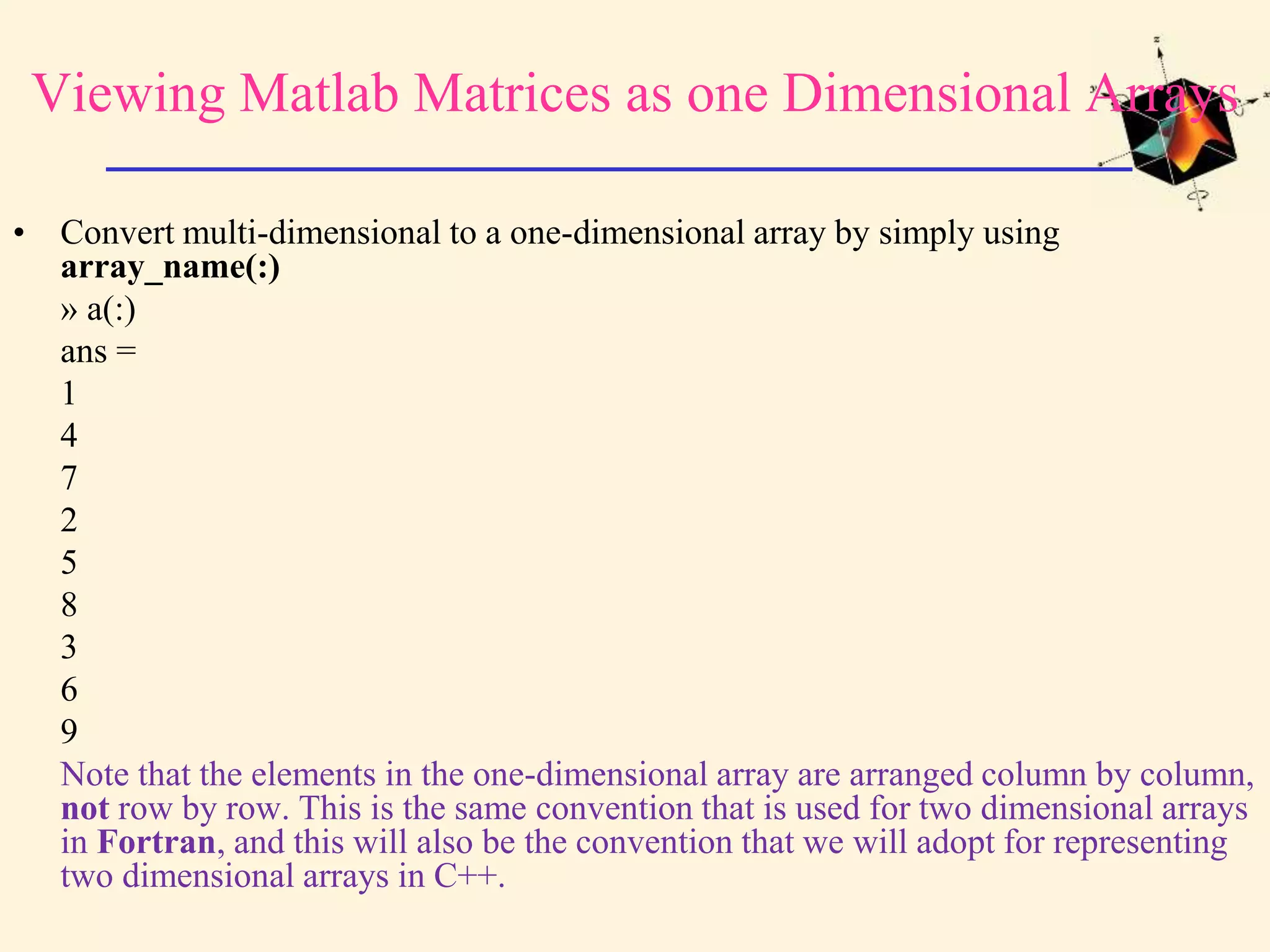
Viewing Matlab Matricesas one Dimensional Arrays • Convert multi-dimensional to a one-dimensional array by simply using array_name(:) » a(:) ans = 1 4 7 2 5 8 3 6 9 Note that the elements in the one-dimensional array are arranged column by column, not row by row. This is the same convention that is used for two dimensional arrays in Fortran, and this will also be the convention that we will adopt for representing two dimensional arrays in C++.
28.
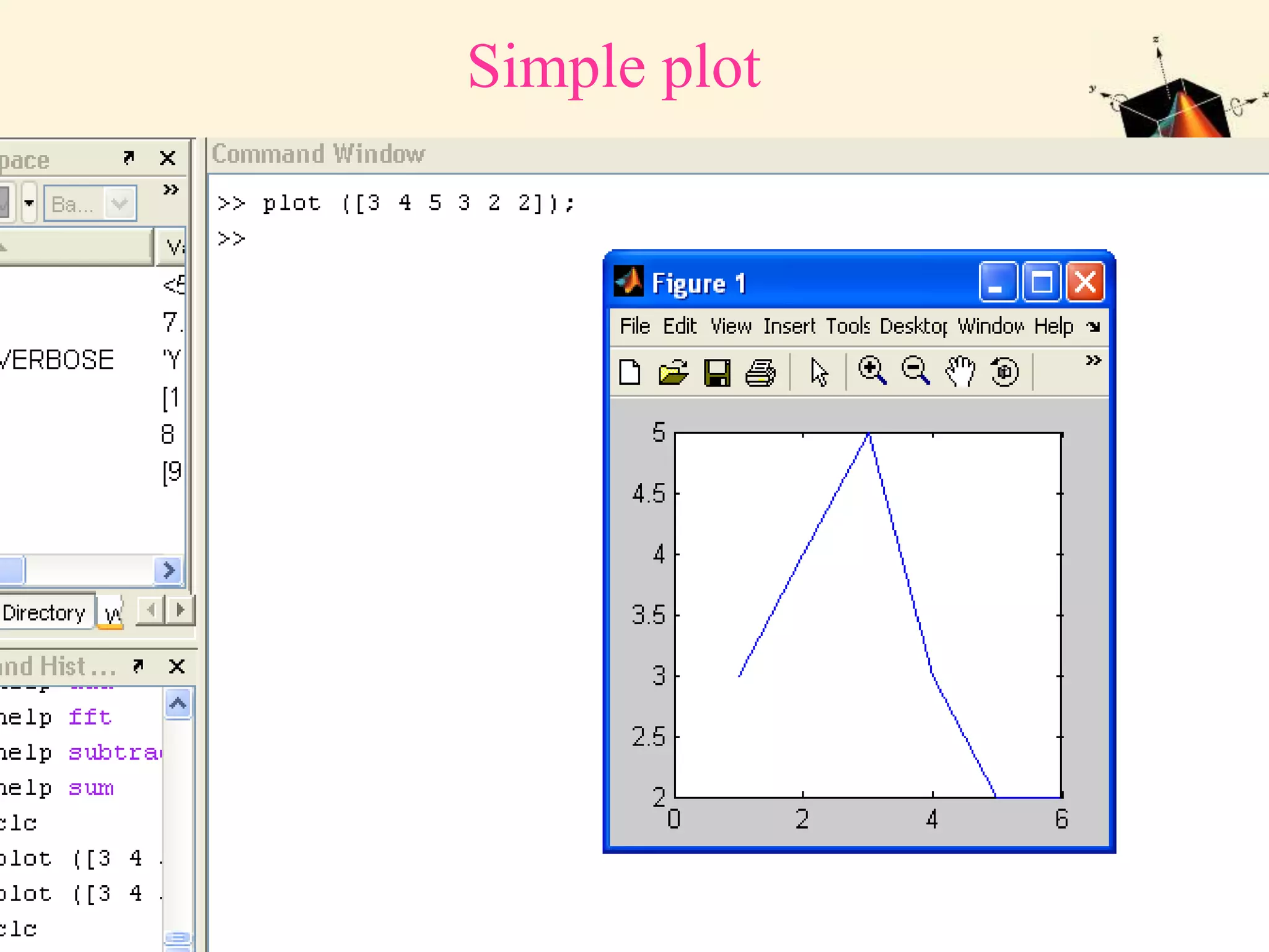
Displaying and Printingin Matlab • To plot an array or display an image, select the figure using: » figure(1); % select the figure to display. » clf % clear the figure from any % previous commands. • and use plot for displaying a one-dimen-sional array: » plot ([3 4 5 3 2 2]); % plots broken-line graph. • or use imagesc for displaying a two dimensional array (image):
29.
One-dimensional random accessiterator (using an index array) [1 5 9 2 6 10 3 7 11 4 8 12] » I=[1 5 8 10]; % indices apply to one-dimensional array a(:) » a(I) ans = 1 6 7 4 – two dimensional iterators » a(1:2,1:3) ans = 1 2 3 5 6 7 .
30.
Working with Memoryin Matlab • To keep track of how memory is allocated, we use whos » b=[34 54 56]; » a=[2 3 56]; » whos Name Size Bytes Class a 1x3 24 double array b 1x3 24 double array Grand total is 6 elements using 48 bytes We may then get rid of unwanted variables using clear » clear a; % removes the variable a from the memory. • We can use clear all to remove all variables from memory (and all functions and mex links) and close all to close all the figures and hence save a lot of memory.
31.
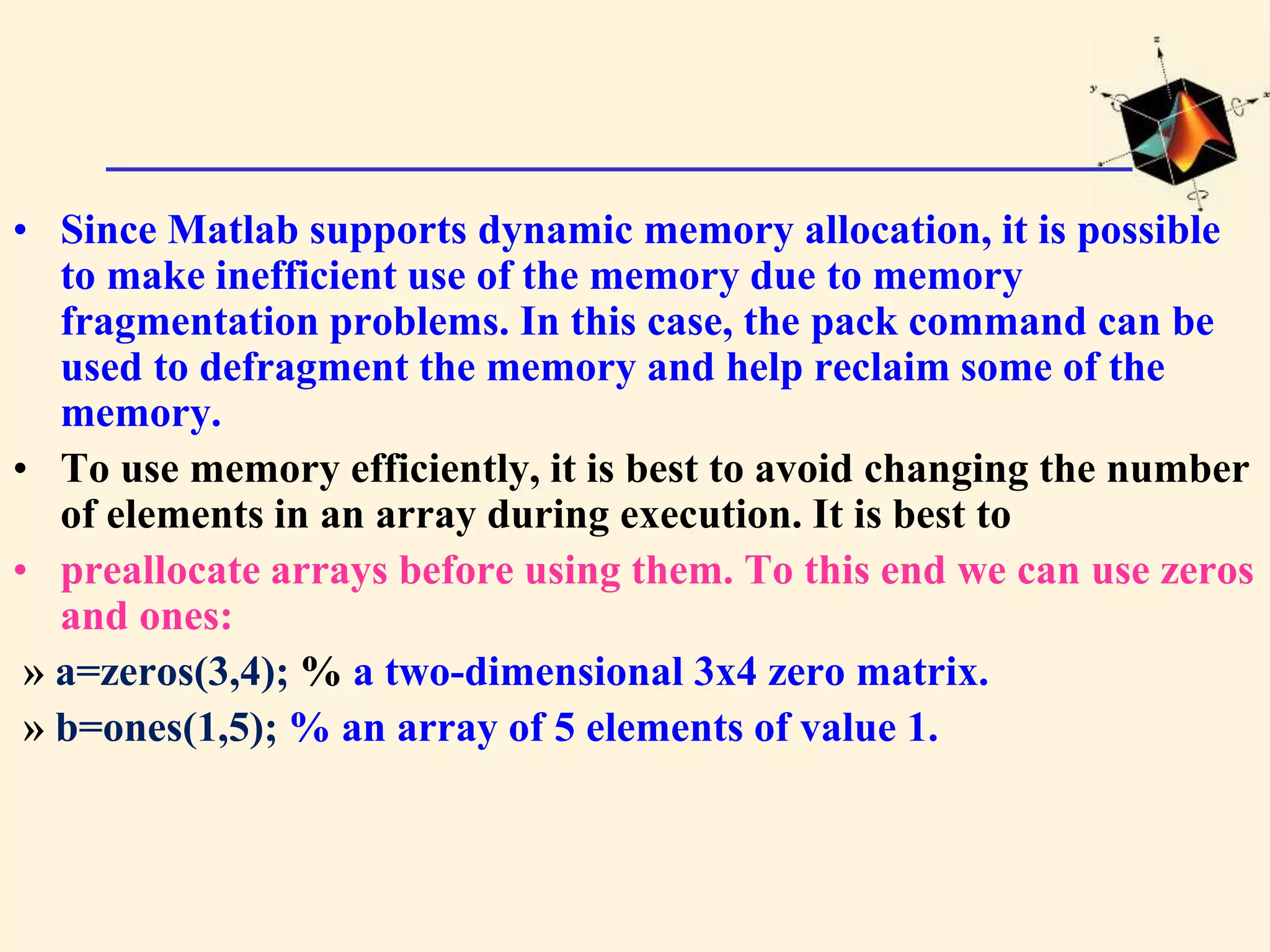
• Since Matlabsupports dynamic memory allocation, it is possible to make inefficient use of the memory due to memory fragmentation problems. In this case, the pack command can be used to defragment the memory and help reclaim some of the memory. • To use memory efficiently, it is best to avoid changing the number of elements in an array during execution. It is best to • preallocate arrays before using them. To this end we can use zeros and ones: » a=zeros(3,4); % a two-dimensional 3x4 zero matrix. » b=ones(1,5); % an array of 5 elements of value 1.
32.
Evaluating one-dimensional functions inMatlab • To evaluate one-dimensional functions in Matlab we need to specify the points at which we would like our function to be evaluated at. • We can use either the built-in colon notation to specify the points » t=-1:0.5:1 t = -1.0000 -0.5000 0 0.5000 1.0000 or use linspace( ) » t=linspace(-2,4,5) % generates 5 points % between -2 and 4 t = -2.0000 -0.5000 1.0000 2.5000 4.0000 or use logspace( )
33.
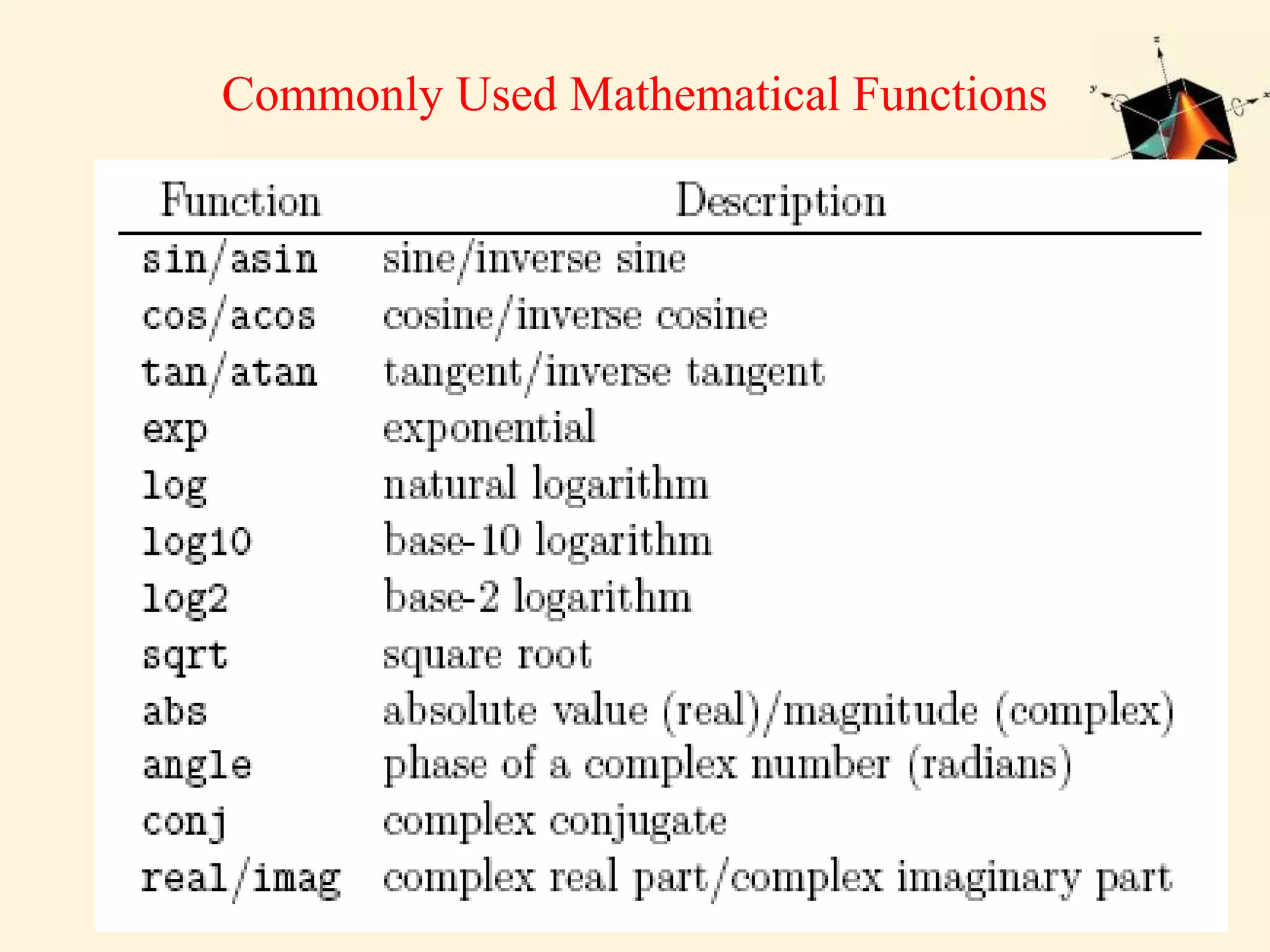
Evaluating one-dimensional functionsin Matlab (contd) • In general, all numbers in Matlab are double. Complex numbers are represented by multiplying the imaginary part by 1i. For example, 1+3j can be represented by 1+1i*3 or 1+3i. • All the well-known mathematical functions are defined in Matlab, and but they apply to to each element in the vector directly. • For example, cos([2 3 4]) is equivalent to [cos(2) cos(3) cos(4)].
34.
Evaluating two-dimensional functions inMatlab • To evaluate two-dimensional functions in Matlab we use the built-in function meshgrid ( ) with the ranges for x and y; eg: » [x,y]=meshgrid(0.1:0.1:0.3, 0.2:0.1:0.4) yields the matrices x and y given by: x = 0.1 0.2 0.3 0.1 0.2 0.3 0.1 0.2 0.3
35.
y = 0.2 0.20.2 0.3 0.3 0.3 0.4 0.4 0.4 • We may then apply any binary operation to x and y provided that we preceed each operation with a period. • For example x.*y represents the matrix where each element of x multiplies each element of y. • Similarly, exp(x.^2+y.^2) represents the matrix resulting from applying exp( ) to the sum of the squares of each of the elements of x and y.
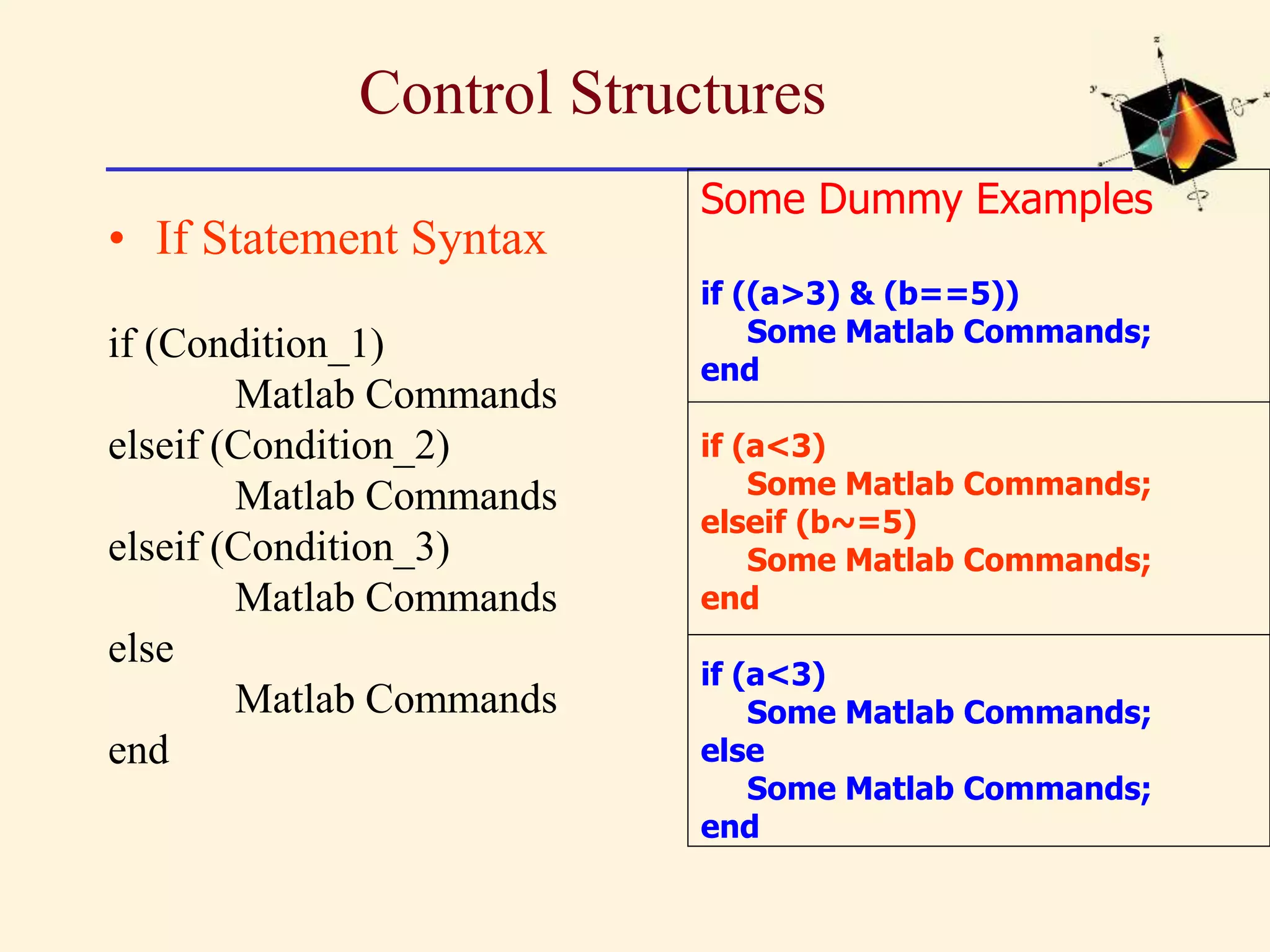
Control Structures • IfStatement Syntax if (Condition_1) Matlab Commands elseif (Condition_2) Matlab Commands elseif (Condition_3) Matlab Commands else Matlab Commands end Some Dummy Examples if ((a>3) & (b==5)) Some Matlab Commands; end if (a<3) Some Matlab Commands; elseif (b~=5) Some Matlab Commands; end if (a<3) Some Matlab Commands; else Some Matlab Commands; end
38.
Control Structures • Forloop syntax for i=Index_Array Matlab Commands end Some Dummy Examples for i=1:100 Some Matlab Commands; end for j=1:3:200 Some Matlab Commands; end for m=13:-0.2:-21 Some Matlab Commands; end for k=[0.1 0.3 -13 12 7 -9.3] Some Matlab Commands; end
39.
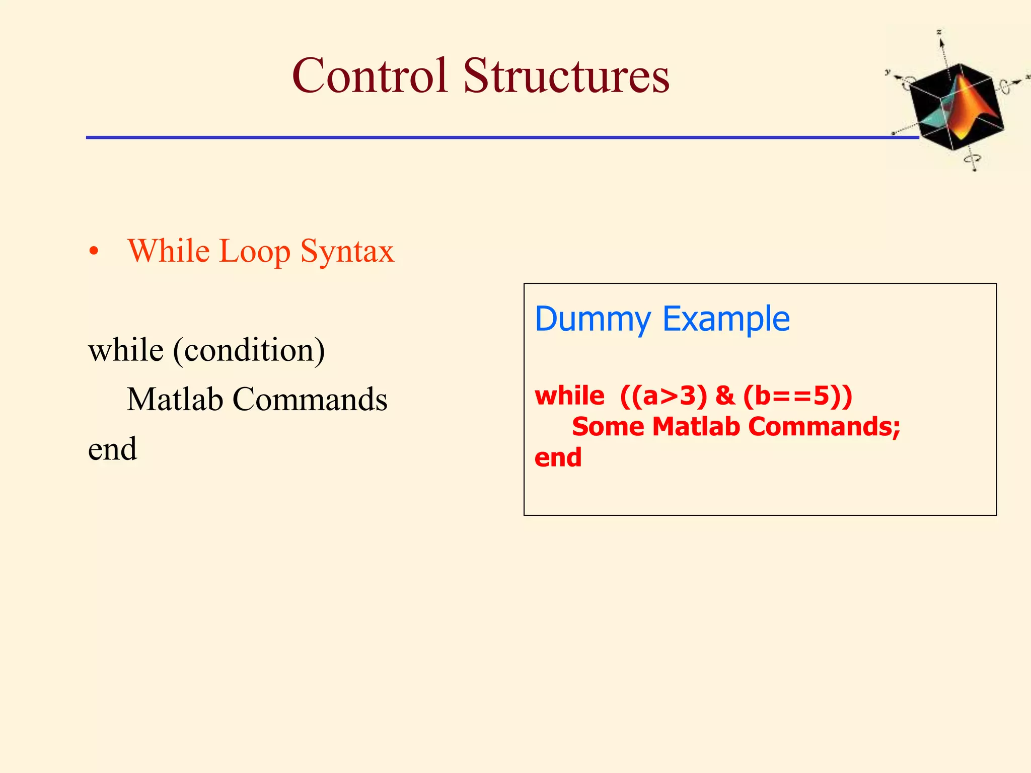
Control Structures • WhileLoop Syntax while (condition) Matlab Commands end Dummy Example while ((a>3) & (b==5)) Some Matlab Commands; end
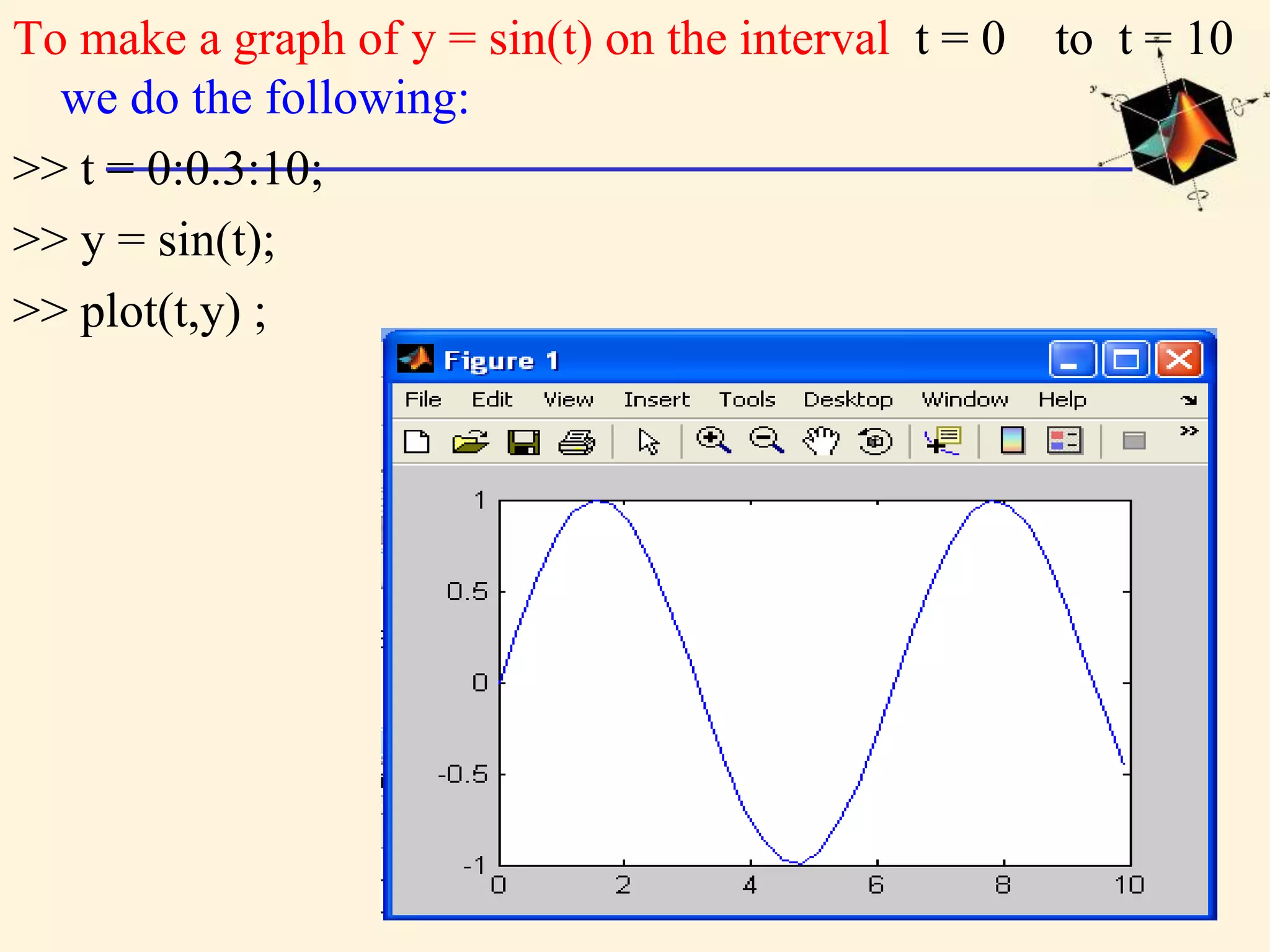
To make agraph of y = sin(t) on the interval t = 0 to t = 10 we do the following: >> t = 0:0.3:10; >> y = sin(t); >> plot(t,y) ;
43.
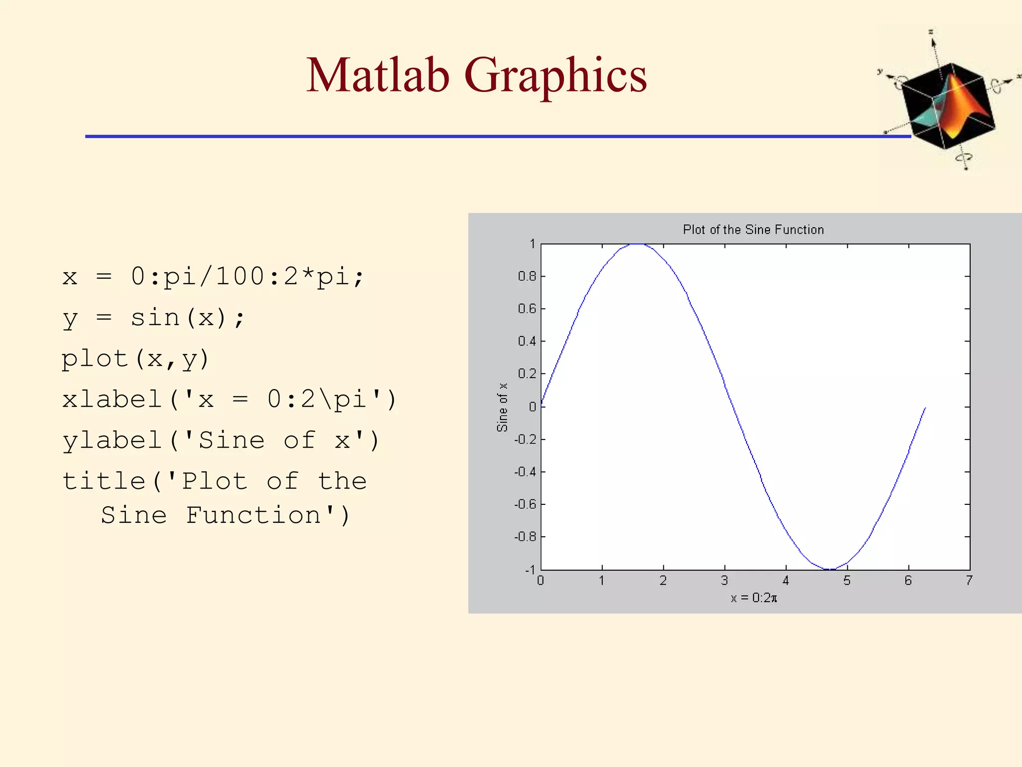
Matlab Graphics x =0:pi/100:2*pi; y = sin(x); plot(x,y) xlabel('x = 0:2pi') ylabel('Sine of x') title('Plot of the Sine Function')
44.
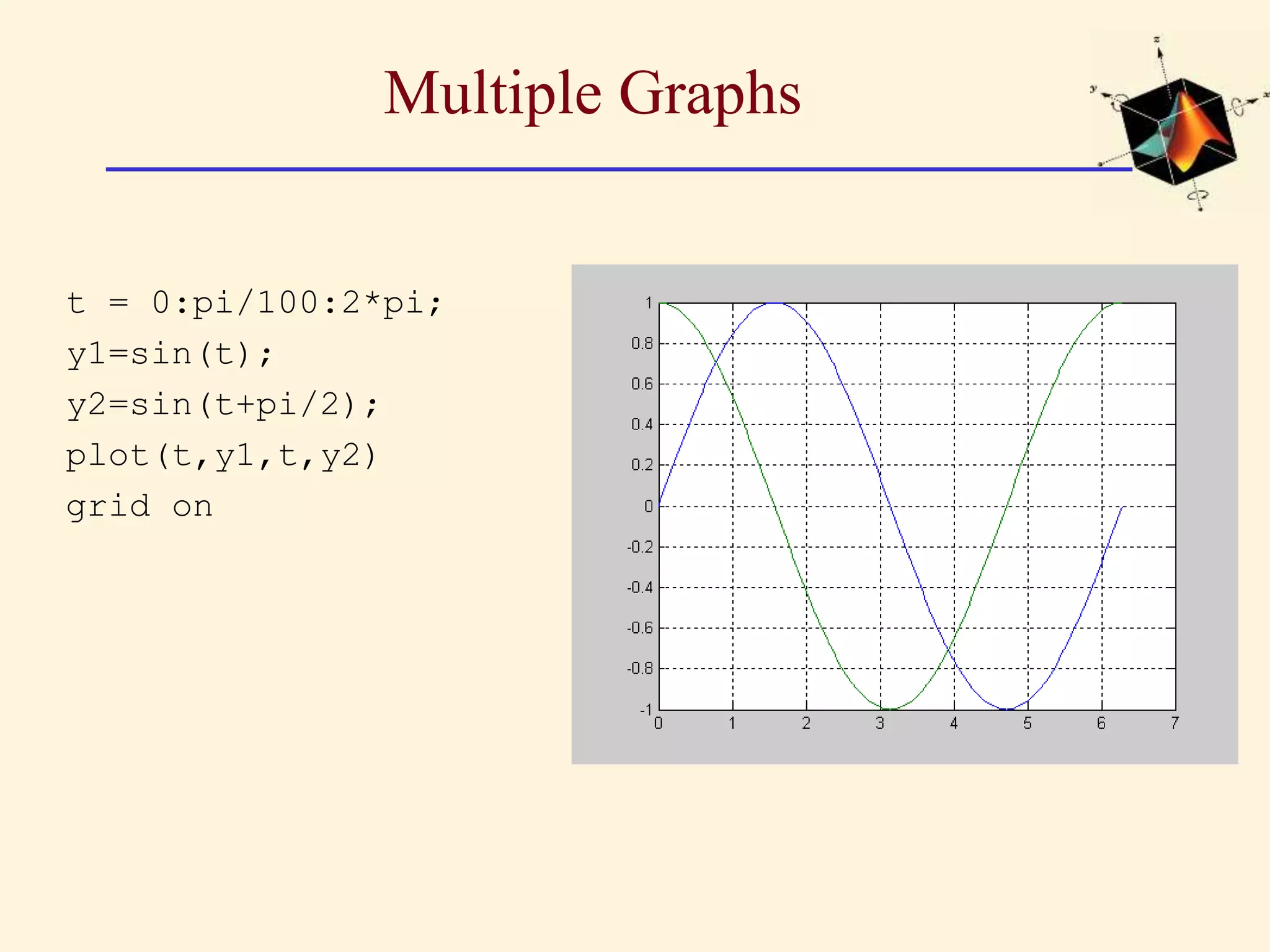
Multiple Graphs t =0:pi/100:2*pi; y1=sin(t); y2=sin(t+pi/2); plot(t,y1,t,y2) grid on
45.
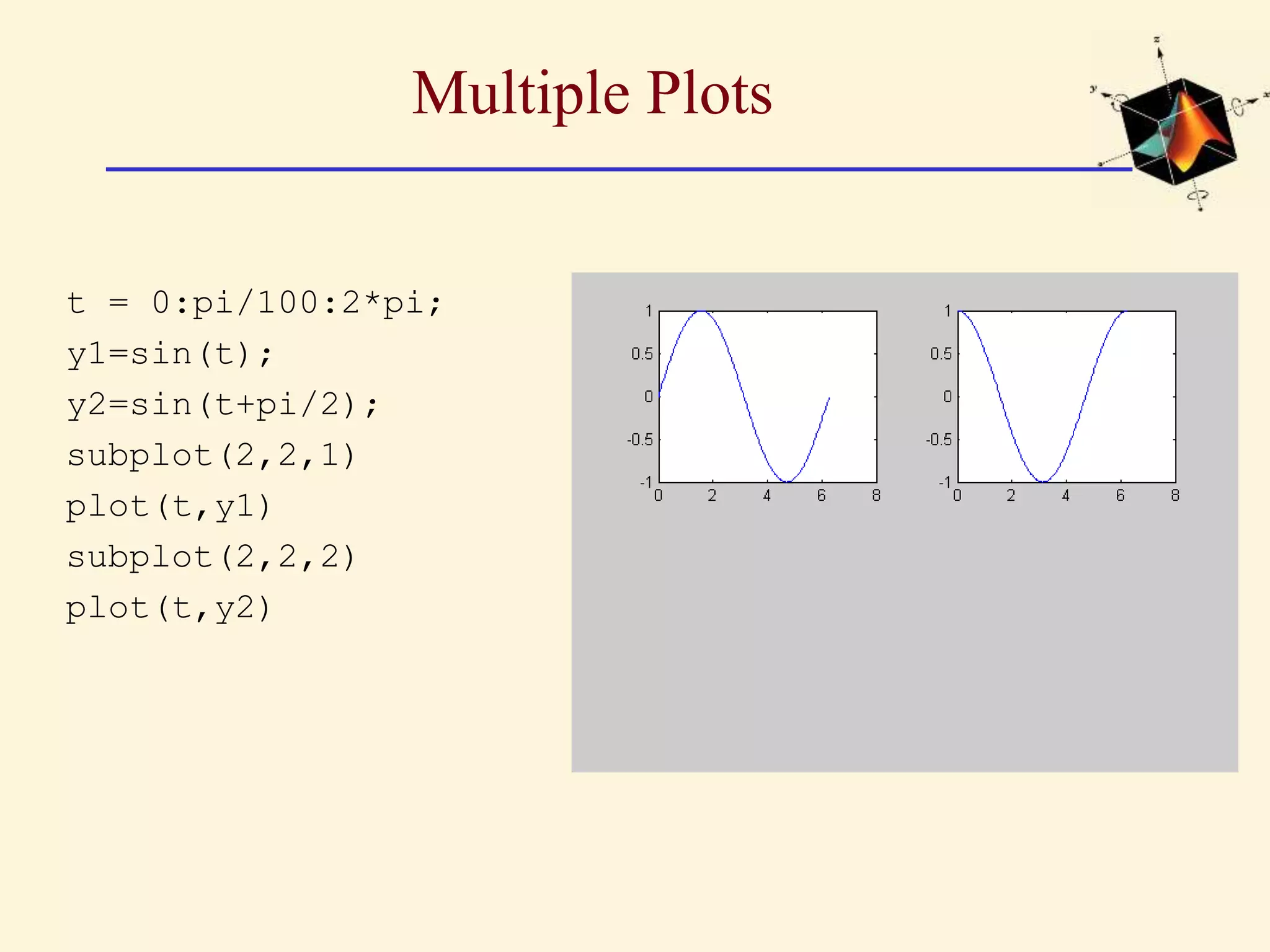
Multiple Plots t =0:pi/100:2*pi; y1=sin(t); y2=sin(t+pi/2); subplot(2,2,1) plot(t,y1) subplot(2,2,2) plot(t,y2)
46.
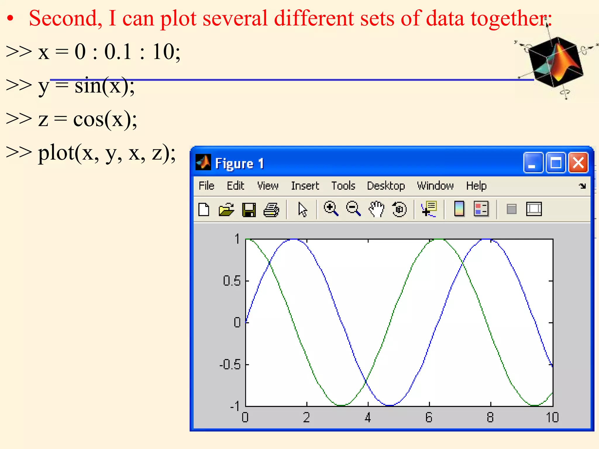
• Second, Ican plot several different sets of data together: >> x = 0 : 0.1 : 10; >> y = sin(x); >> z = cos(x); >> plot(x, y, x, z);
47.
• Another usefulcommand is axis, which lets you control the size of the axes. If I've already created the plot with both sine and cosine functions, I can resize it by typing >> axis([-5, 15, -3, 3]); which changes the plotting window so it looks like this:
48.
• f (x)=sin(x)3 +cos(3x) • over one period syms x; ezplot(sin(x)^3+ cos(3*x), [-pi pi], 1); grid on;
49.
Continuous and Discretetime plots k=0:20; y=binopdf(k,20,0.5); plot(k,y) k=0:20; y=binopdf(k,20,0.5); stem(k,y)
Using Matlab Editors •Very small programs can be typed and executed in command window. • Large programs on other hand can be used the Matlab editor. • The complete program can be typed in the Matlab editor and saved as ‘file_name.m’, and can be retrieved when-ever necessary. • You can execute either directly from editor window or type the file name in the command window and press the enter button.
55.
Creating, Saving, andExecuting a Script File % CIRCLE - A script file to draw a pretty circle function [x, y] = prettycirclefn(r) % CIRCLE - A script file to draw a pretty circle % Input: r = specified radius % Output: [x, y] = the x and y coordinates angle = linspace(0, 2*pi, 360); x = r * cos(angle); y = r * sin(angle); plot(x,y) axis('equal') ylabel('y') xlabel('x') title(['Radius r =',num2str(r)]) grid on
56.
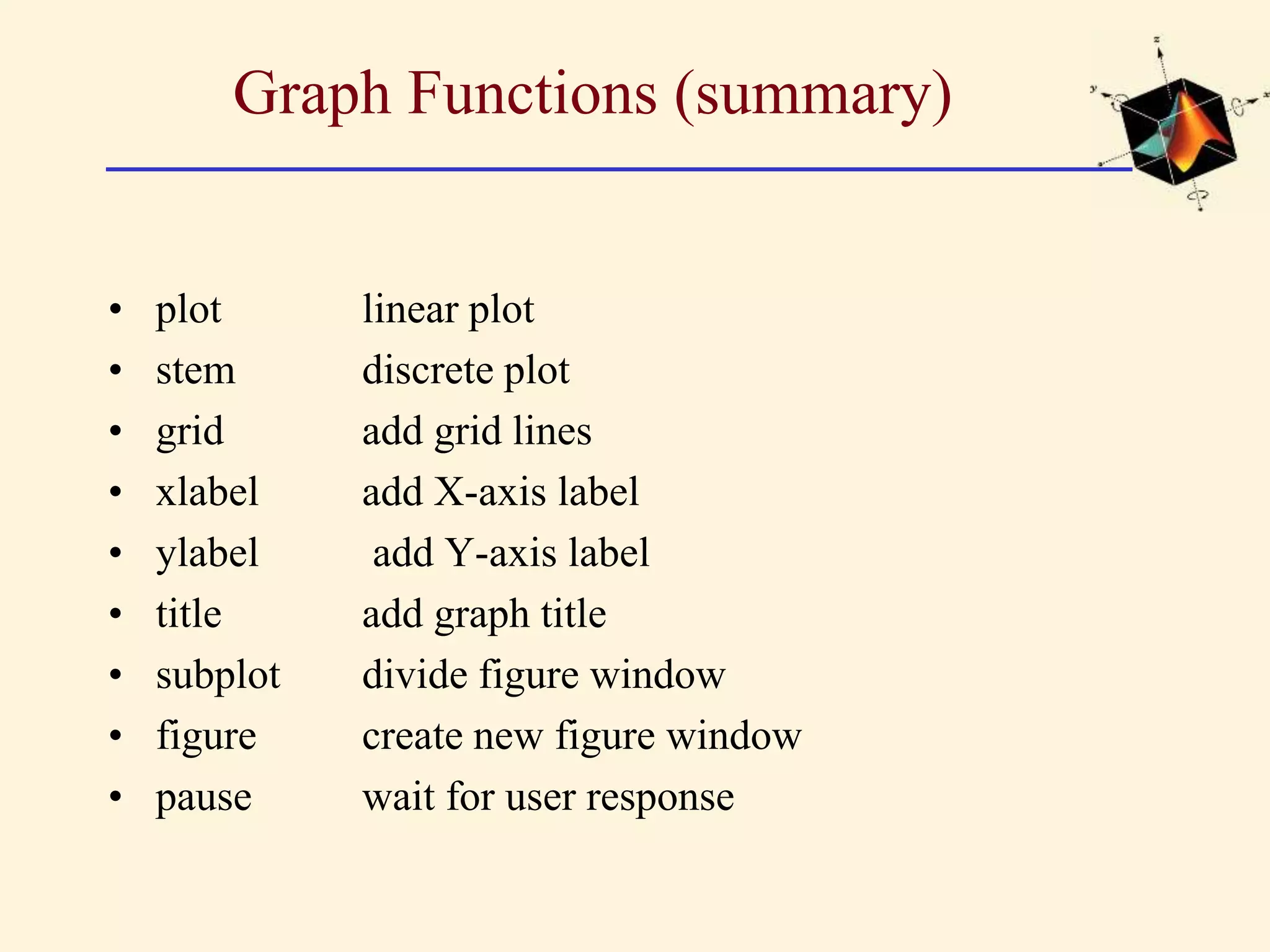
Graph Functions (summary) •plot linear plot • stem discrete plot • grid add grid lines • xlabel add X-axis label • ylabel add Y-axis label • title add graph title • subplot divide figure window • figure create new figure window • pause wait for user response
57.
• clc: clearcommand window • clear all: clear all variables in workspace window • close all: closes all previous figure windows


![Definition of Vectors & Matrices • MATLAB is based on matrix and vector algebra; even scalars are treated as 1x1 matrices. Therefore, vector and matrix operations are as simple as common calculator operations. • Vectors can be defined in two ways. * The first method is used for arbitrary elements: v = [1 3 5 7]; creates a 1x4 vector with elements 1, 3, 5 and 7. * Note that commas could have been used in place of spaces to separate the elements. that is v=[1,3,5,7]; • Additional elements can be added to the vector: v(5) = 8; yields the vector v = [1 3 5 7 8].](https://image.slidesharecdn.com/matlabtutorial-230107051626-056fcb8b/75/Matlab-Tutorial-ppt-15-2048.jpg)
![• Previously defined vectors can be used to define a new vector. For example, with ‘v’ defined above a = [9 10]; b = [v a]; creates the vector b = [1 3 5 7 8 9 10].](https://image.slidesharecdn.com/matlabtutorial-230107051626-056fcb8b/75/Matlab-Tutorial-ppt-16-2048.jpg)

![* Matrices are defined by entering the elements row by row: M = [1 2 4; 3 6 8; 2 6 5]; creates the matrix * Transpose of M is denoted by M’, and displays as *The inverse of M is M-1 denoted in Matlab as M^-1and displays as * M(2,3) displays the element of second row and third column](https://image.slidesharecdn.com/matlabtutorial-230107051626-056fcb8b/75/Matlab-Tutorial-ppt-18-2048.jpg)
![Special Matrices • null matrix: M = [ ]; • nxm matrix of zeros: M = zeros(n,m); nxm matrix of ones: M = ones(n,m); nxn identity matrix: M = eye(n);](https://image.slidesharecdn.com/matlabtutorial-230107051626-056fcb8b/75/Matlab-Tutorial-ppt-23-2048.jpg)
![• Comments in Matlab must be proceeded by % % This is a comment in Matlab. • To define a function in Matlab, we first create a function with the name of the function. *We then define the function in the file. *For example, the Matlab documentation recommends stat.m written as: function [mean,stdev] = stat(x) % This comment is printed out with help stat n = length(x); % assumes that x is a vector. mean = sum(x) / n; % sum adds up all elements. stdev = sqrt(sum((x - mean).^2)/n);](https://image.slidesharecdn.com/matlabtutorial-230107051626-056fcb8b/75/Matlab-Tutorial-ppt-26-2048.jpg)
![Displaying and Printing in Matlab • To plot an array or display an image, select the figure using: » figure(1); % select the figure to display. » clf % clear the figure from any % previous commands. • and use plot for displaying a one-dimen-sional array: » plot ([3 4 5 3 2 2]); % plots broken-line graph. • or use imagesc for displaying a two dimensional array (image):](https://image.slidesharecdn.com/matlabtutorial-230107051626-056fcb8b/75/Matlab-Tutorial-ppt-28-2048.jpg)
![One-dimensional random access iterator (using an index array) [1 5 9 2 6 10 3 7 11 4 8 12] » I=[1 5 8 10]; % indices apply to one-dimensional array a(:) » a(I) ans = 1 6 7 4 – two dimensional iterators » a(1:2,1:3) ans = 1 2 3 5 6 7 .](https://image.slidesharecdn.com/matlabtutorial-230107051626-056fcb8b/75/Matlab-Tutorial-ppt-29-2048.jpg)
![Working with Memory in Matlab • To keep track of how memory is allocated, we use whos » b=[34 54 56]; » a=[2 3 56]; » whos Name Size Bytes Class a 1x3 24 double array b 1x3 24 double array Grand total is 6 elements using 48 bytes We may then get rid of unwanted variables using clear » clear a; % removes the variable a from the memory. • We can use clear all to remove all variables from memory (and all functions and mex links) and close all to close all the figures and hence save a lot of memory.](https://image.slidesharecdn.com/matlabtutorial-230107051626-056fcb8b/75/Matlab-Tutorial-ppt-30-2048.jpg)

![Evaluating one-dimensional functions in Matlab (contd) • In general, all numbers in Matlab are double. Complex numbers are represented by multiplying the imaginary part by 1i. For example, 1+3j can be represented by 1+1i*3 or 1+3i. • All the well-known mathematical functions are defined in Matlab, and but they apply to to each element in the vector directly. • For example, cos([2 3 4]) is equivalent to [cos(2) cos(3) cos(4)].](https://image.slidesharecdn.com/matlabtutorial-230107051626-056fcb8b/75/Matlab-Tutorial-ppt-33-2048.jpg)
![Evaluating two-dimensional functions in Matlab • To evaluate two-dimensional functions in Matlab we use the built-in function meshgrid ( ) with the ranges for x and y; eg: » [x,y]=meshgrid(0.1:0.1:0.3, 0.2:0.1:0.4) yields the matrices x and y given by: x = 0.1 0.2 0.3 0.1 0.2 0.3 0.1 0.2 0.3](https://image.slidesharecdn.com/matlabtutorial-230107051626-056fcb8b/75/Matlab-Tutorial-ppt-34-2048.jpg)


![Control Structures • For loop syntax for i=Index_Array Matlab Commands end Some Dummy Examples for i=1:100 Some Matlab Commands; end for j=1:3:200 Some Matlab Commands; end for m=13:-0.2:-21 Some Matlab Commands; end for k=[0.1 0.3 -13 12 7 -9.3] Some Matlab Commands; end](https://image.slidesharecdn.com/matlabtutorial-230107051626-056fcb8b/75/Matlab-Tutorial-ppt-38-2048.jpg)

![• Another useful command is axis, which lets you control the size of the axes. If I've already created the plot with both sine and cosine functions, I can resize it by typing >> axis([-5, 15, -3, 3]); which changes the plotting window so it looks like this:](https://image.slidesharecdn.com/matlabtutorial-230107051626-056fcb8b/75/Matlab-Tutorial-ppt-47-2048.jpg)
![• f (x)=sin (x)3 +cos(3x) • over one period syms x; ezplot(sin(x)^3+ cos(3*x), [-pi pi], 1); grid on;](https://image.slidesharecdn.com/matlabtutorial-230107051626-056fcb8b/75/Matlab-Tutorial-ppt-48-2048.jpg)

![Creating, Saving, and Executing a Script File % CIRCLE - A script file to draw a pretty circle function [x, y] = prettycirclefn(r) % CIRCLE - A script file to draw a pretty circle % Input: r = specified radius % Output: [x, y] = the x and y coordinates angle = linspace(0, 2*pi, 360); x = r * cos(angle); y = r * sin(angle); plot(x,y) axis('equal') ylabel('y') xlabel('x') title(['Radius r =',num2str(r)]) grid on](https://image.slidesharecdn.com/matlabtutorial-230107051626-056fcb8b/75/Matlab-Tutorial-ppt-55-2048.jpg)