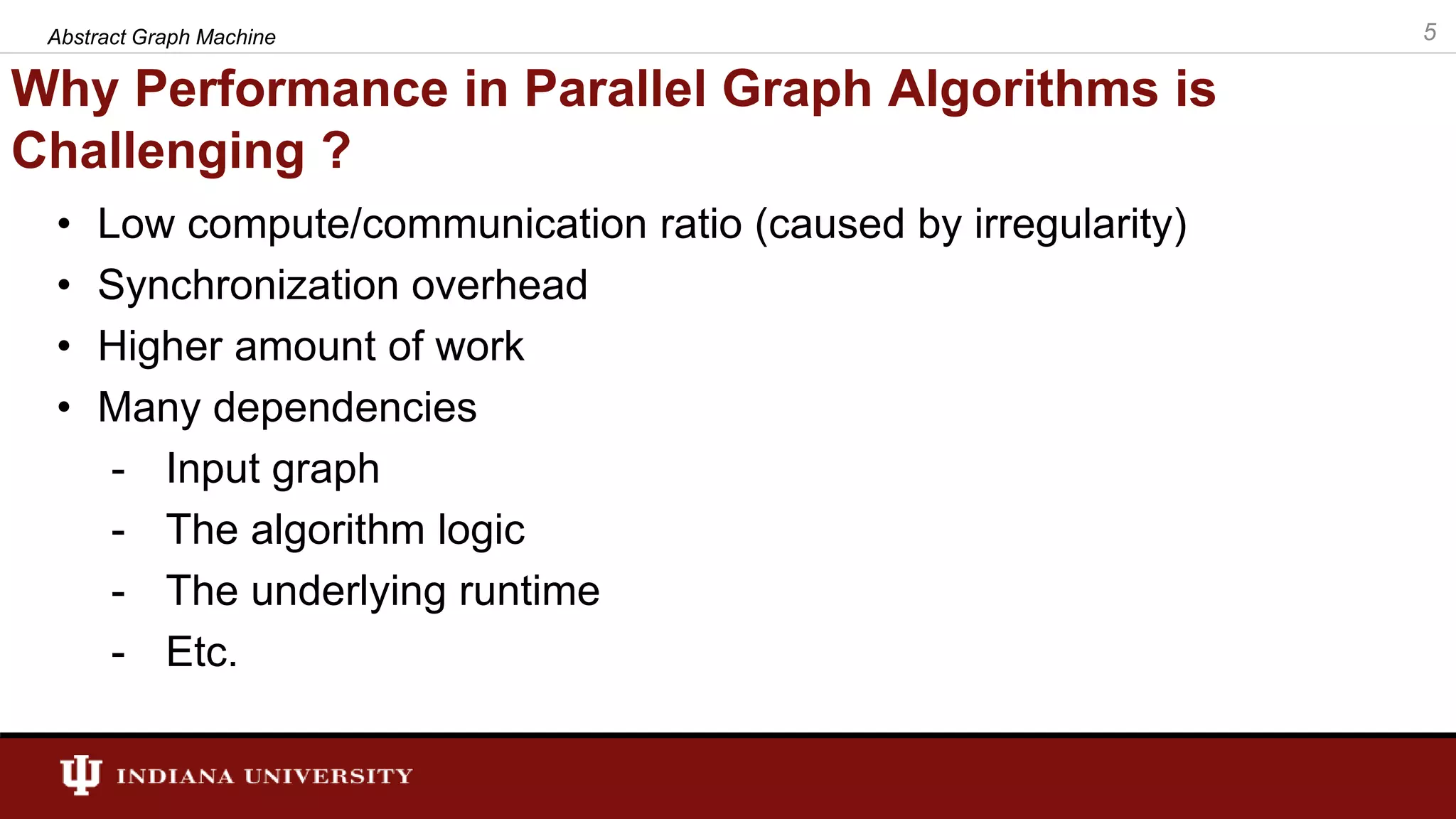
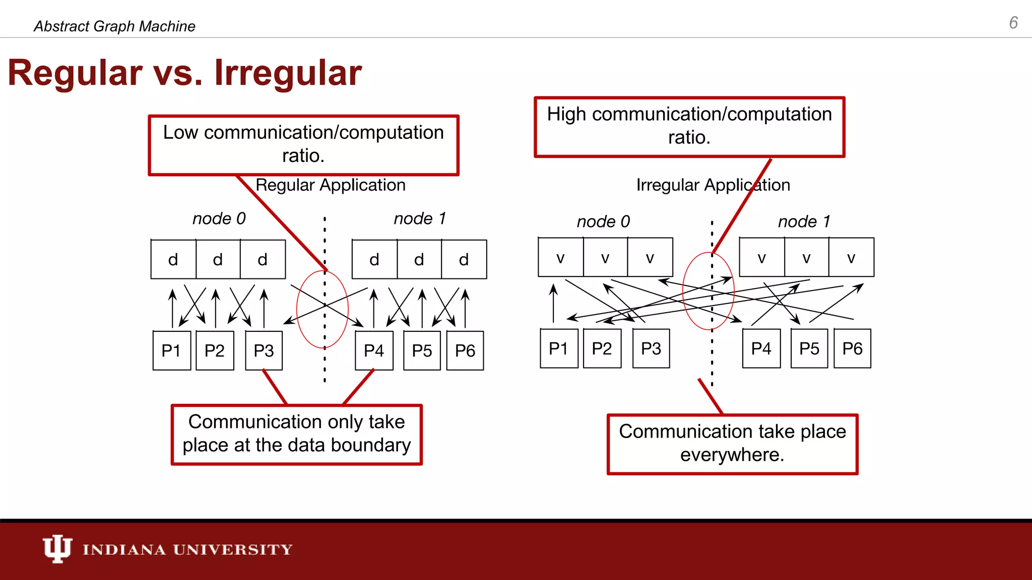
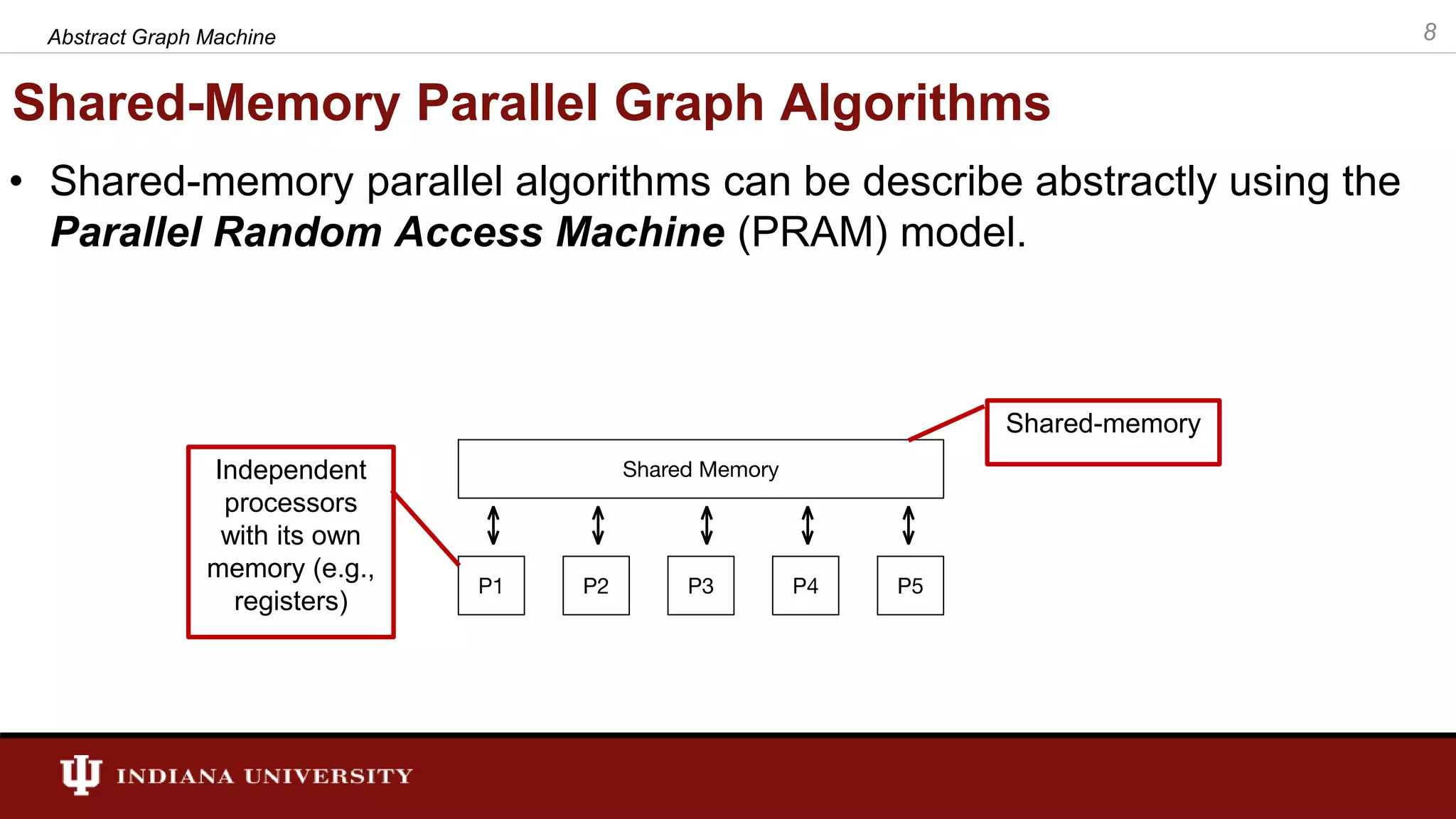
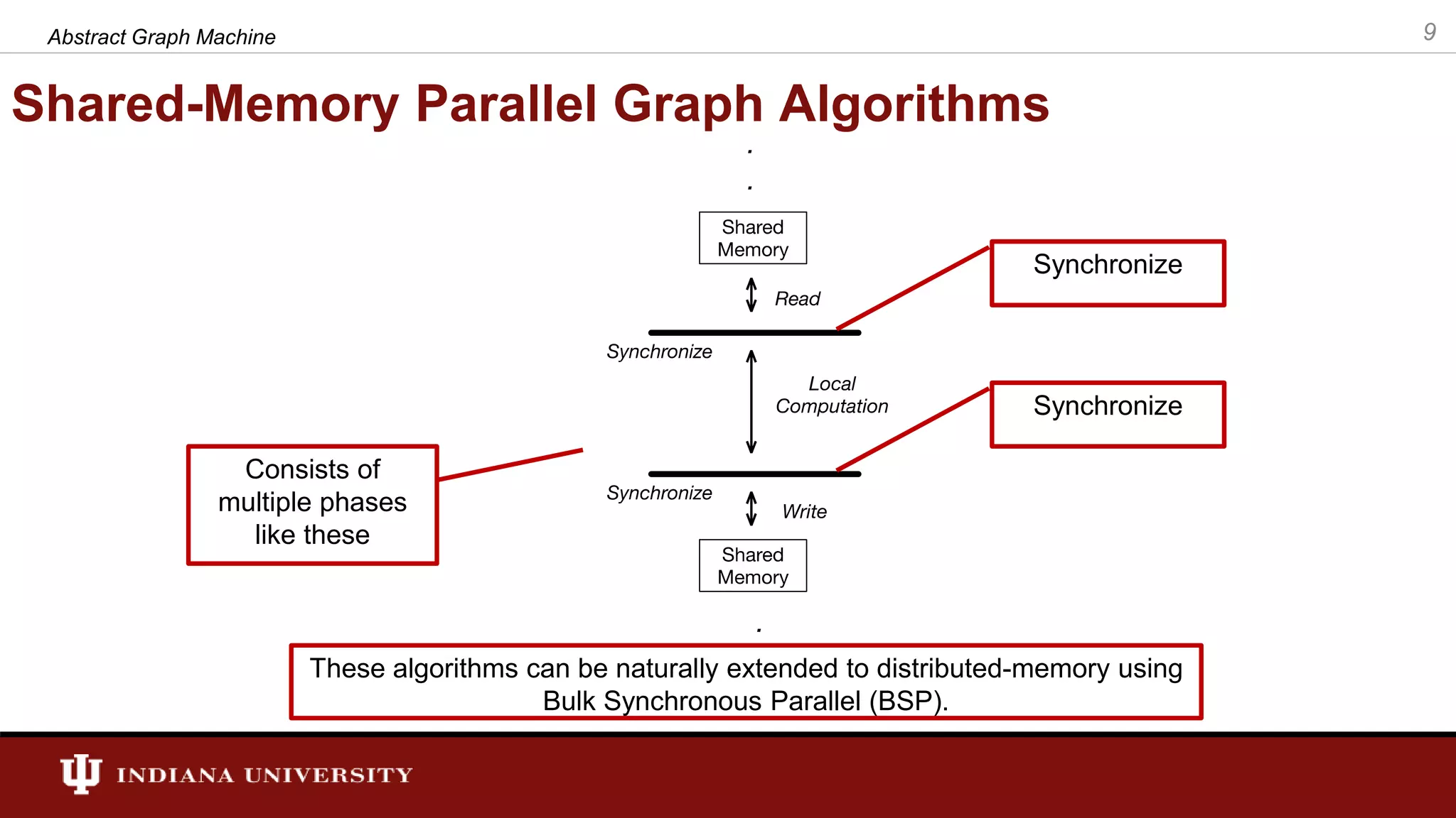
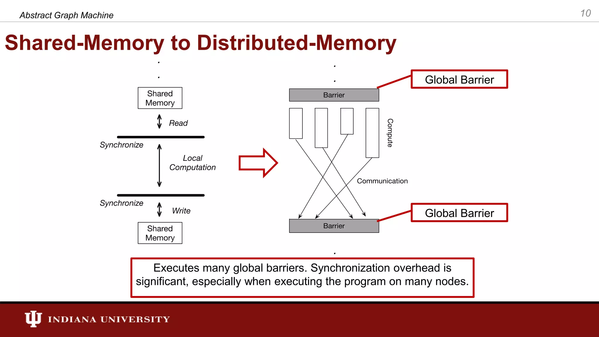
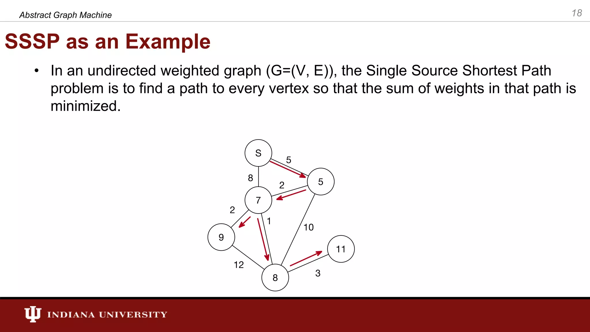
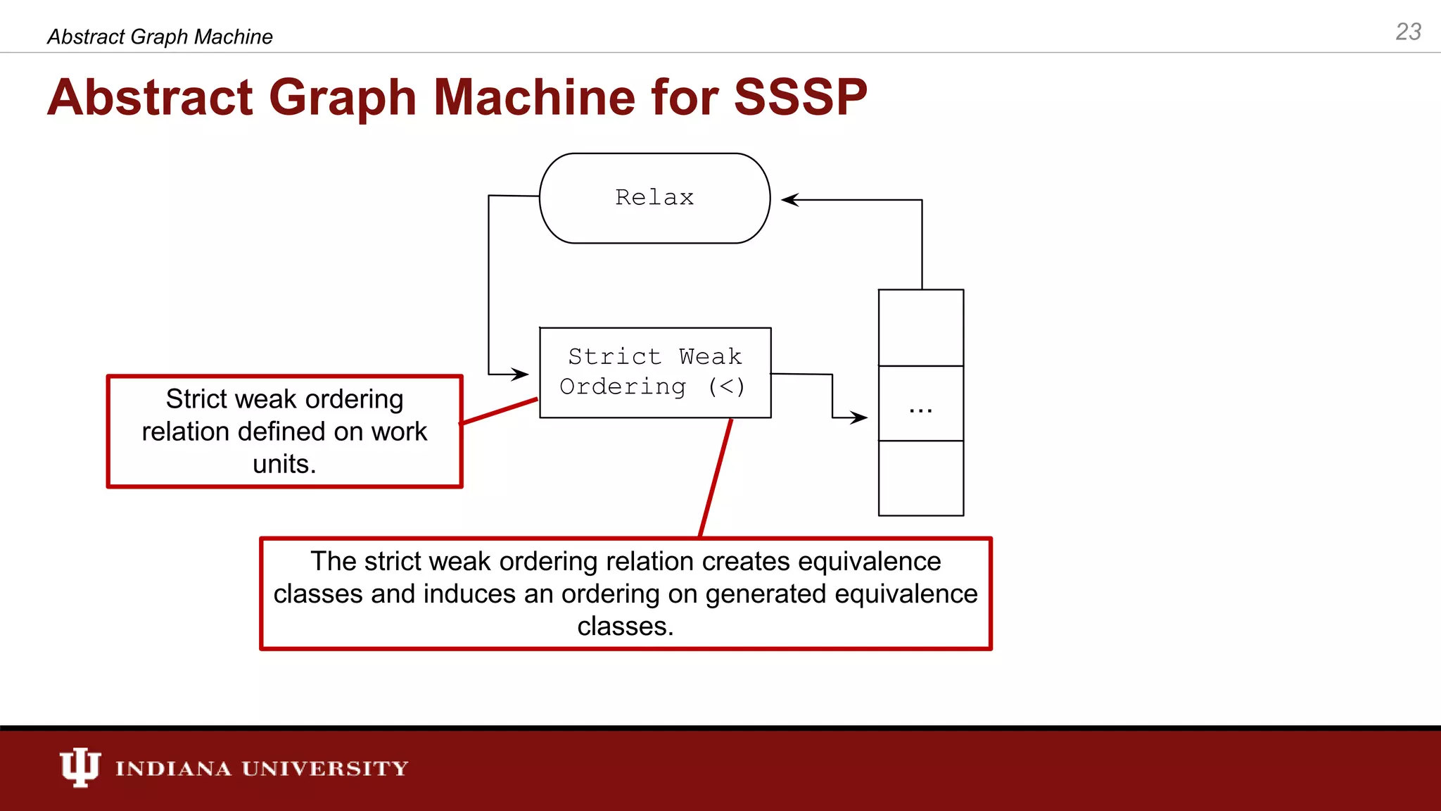
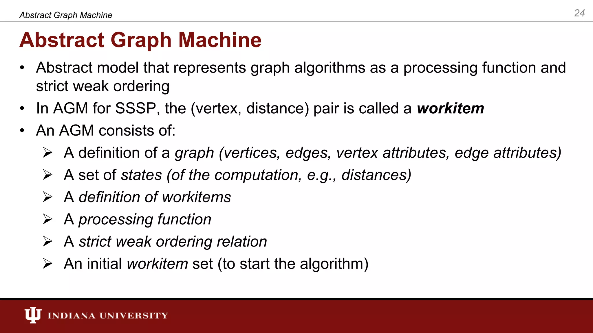
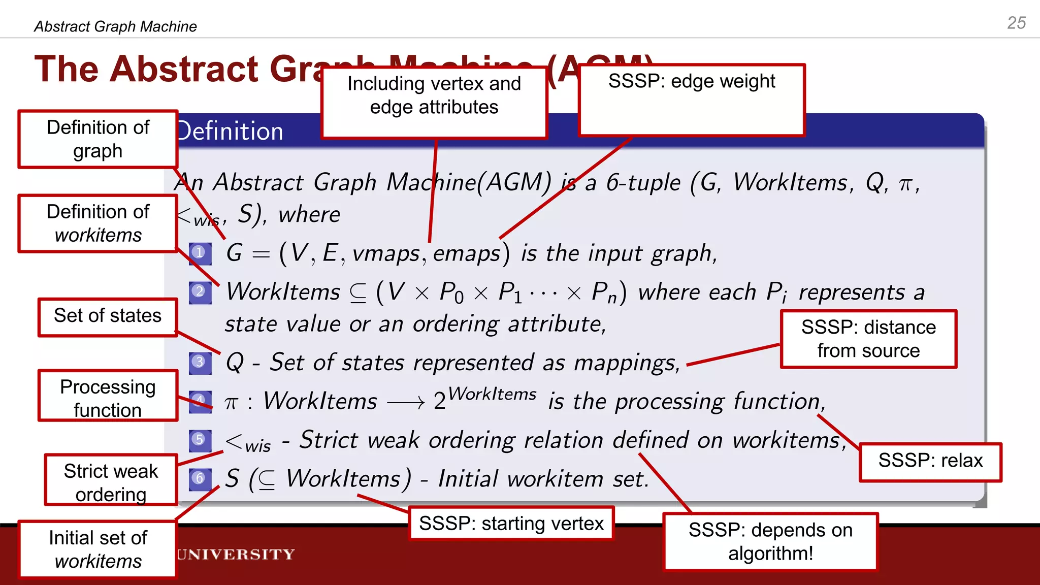
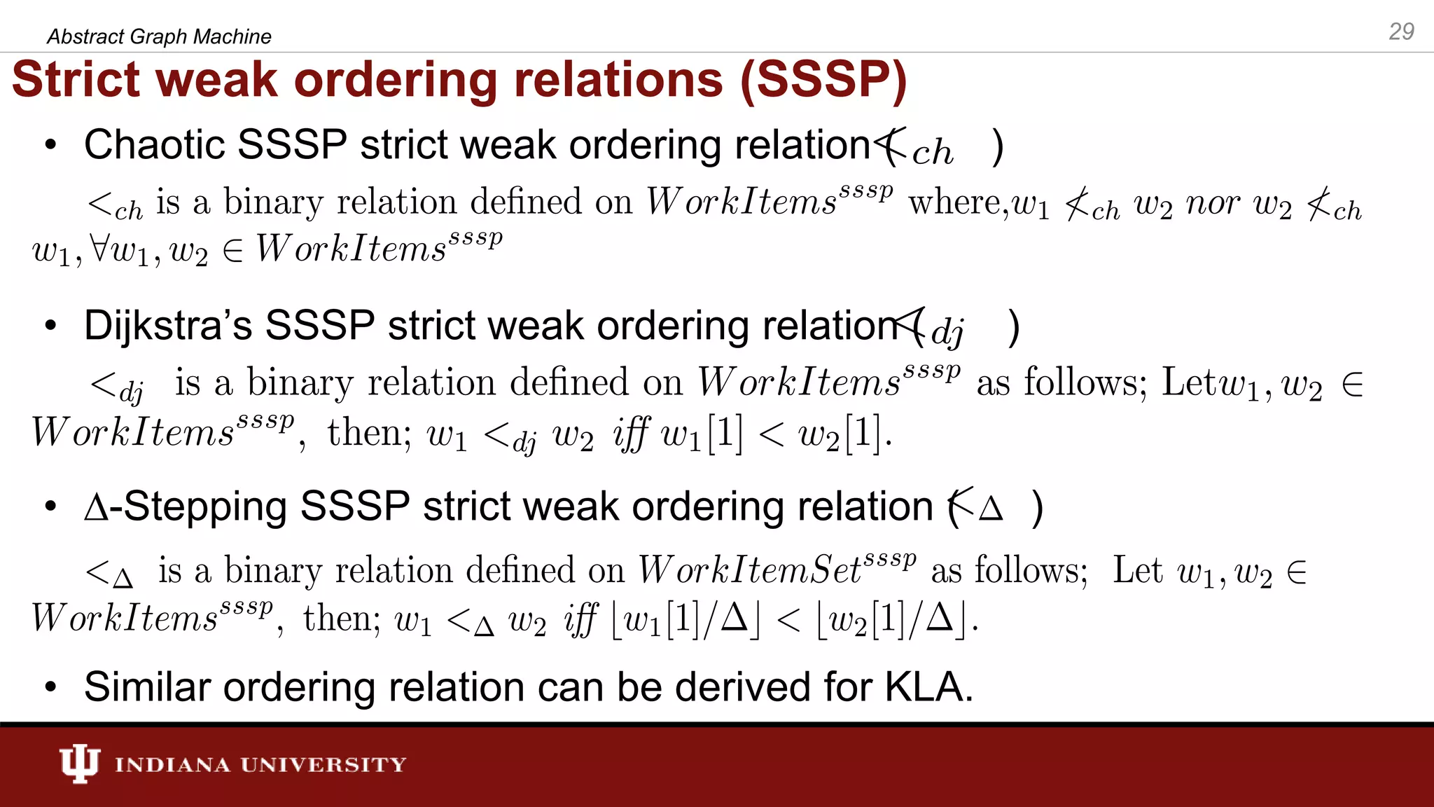
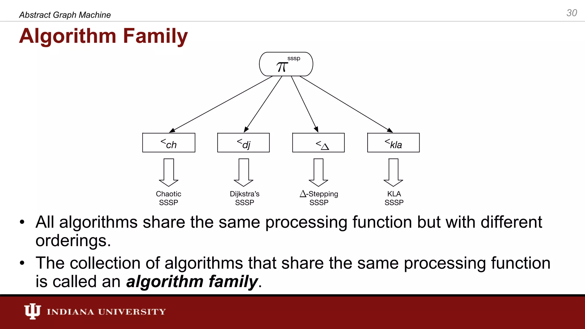
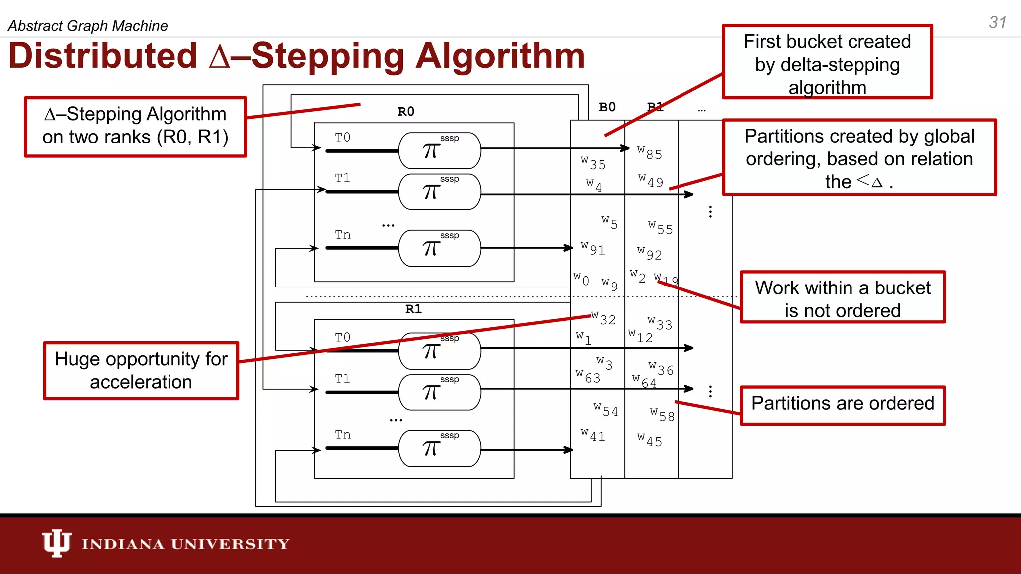
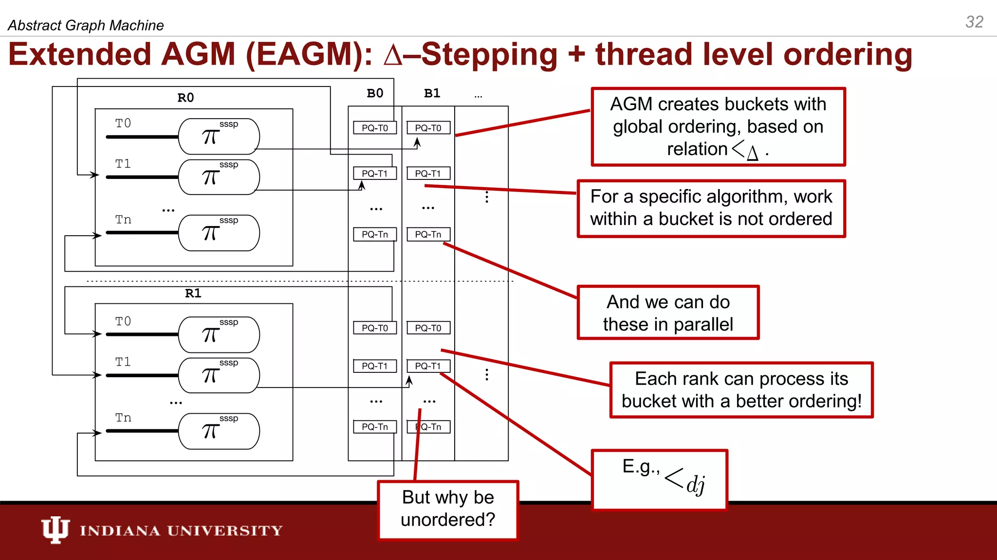
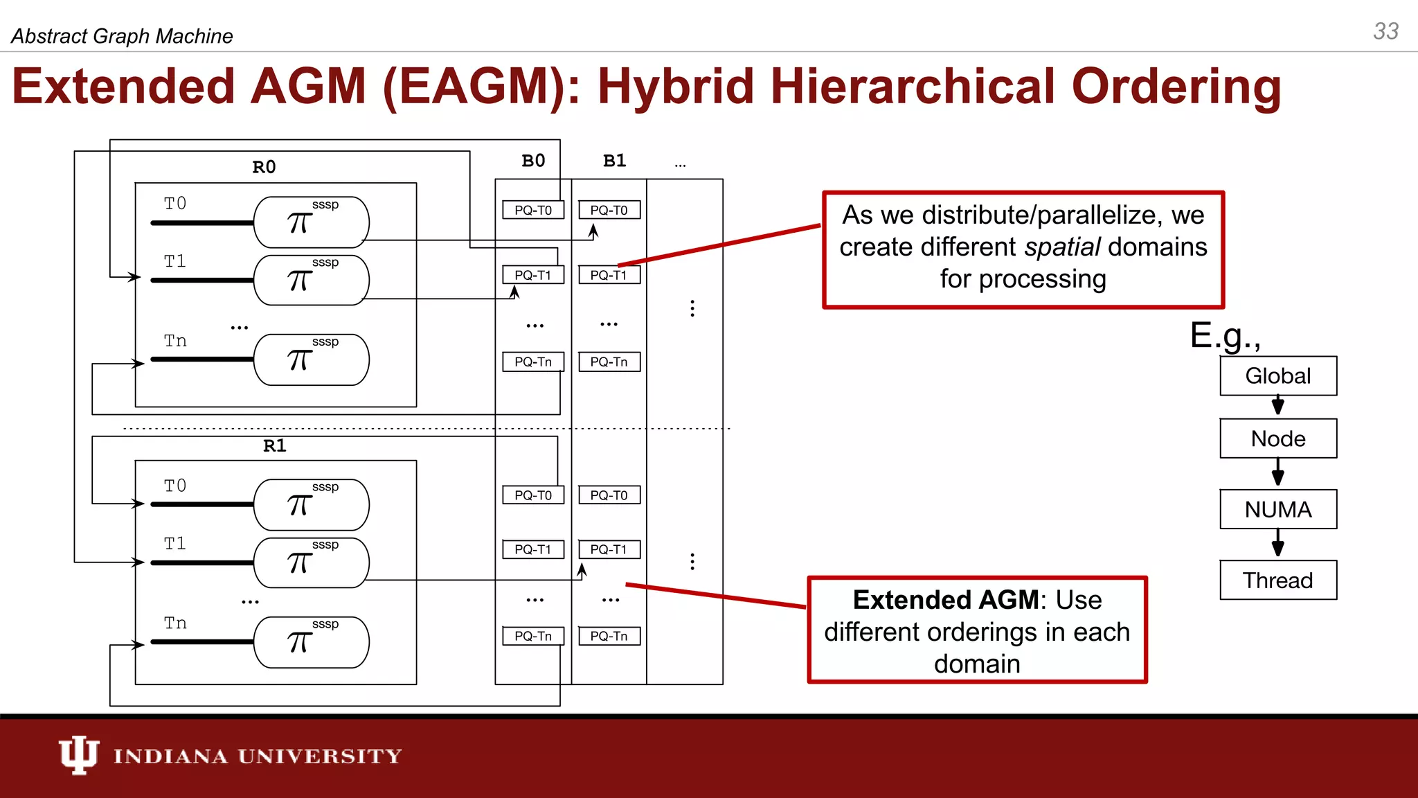
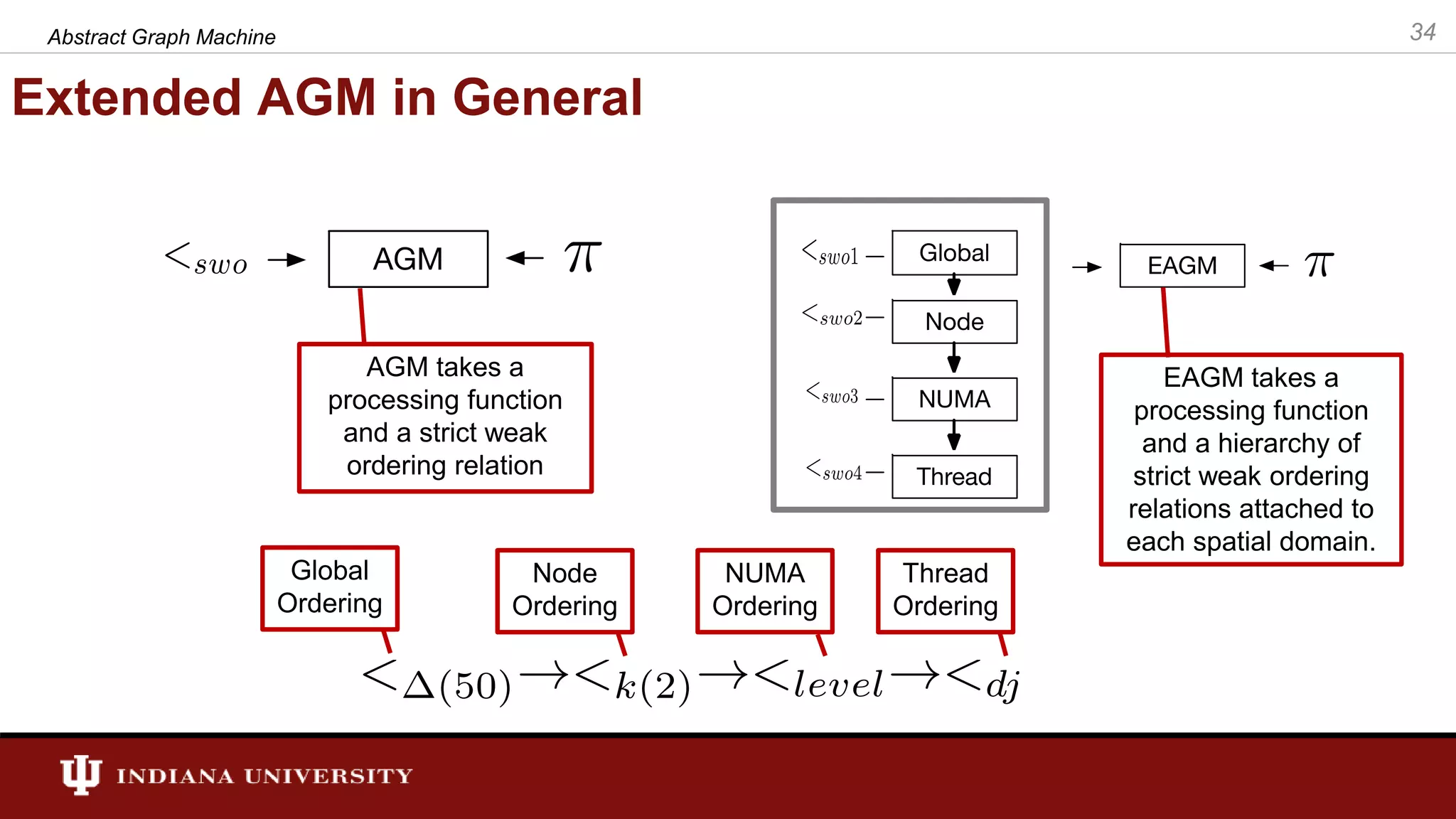
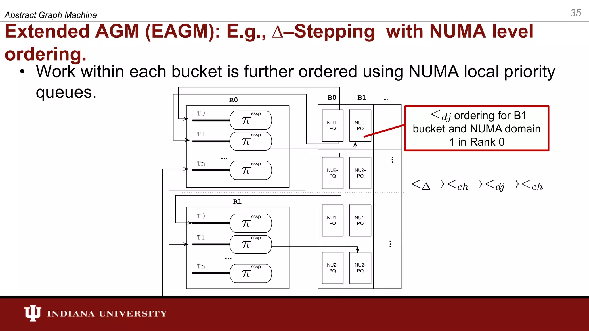
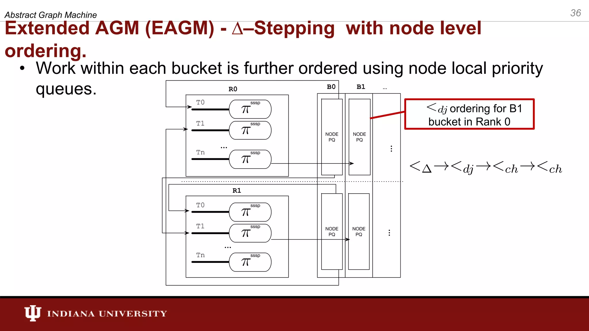
The document discusses the modeling of asynchronous distributed-memory parallel graph algorithms, focusing on the Abstract Graph Machine (AGM) and Extended Abstract Graph Machine (EAGM) frameworks. These frameworks address challenges such as synchronization overhead and communication ratios in existing parallel graph algorithms by introducing work items and strict weak ordering relations to manage processing efficiently. Key algorithms like Dijkstra's and Delta-stepping are explored, demonstrating how different orderings can impact performance in distributed environments.

![Algorithms void Chaotic(Graph g, Vertex source) { For each Vertex v in G { state[v] <- INFINITY; } Relax(source, 0); } void Relax(Vertex v, Distance d) { If (d < state[v]) { state[v] <- d; For each edge e of v { Vertex u = target_vertex(e); Relax(u, d+weight[e]); } } } void Dijkstra(Graph g, Vertex source) { For each Vertex v in G { state[v] <- INFINITY; } pq.insert(<source, 0>); While pq is not empty { <v, d> = vertex-distance pair with minimum distance in pq; Relax(v, d); } } void Relax(Vertex v, Distance d) { If (d < state[v]) { state[v] <- d; For each edge e of v { Vertex u = target_vertex(e); pq.insert(<u, d+weight[e]>); } } } void -Stepping(Graph g, Vertex source) { For each Vertex v in G { state[v] <- INFINITY; } insert <source, 0> to appropriate bucket from buckets; While all buckets are not empty { bucket = smallest non-empty bucket in buckets; For each <v, d> in bucket { Relax(v, d); } } } void Relax(Vertex v, Distance d) { If (d < state[v]) { state[v] <- d For each edge e of v { Vertex u = target_vertex(e); insert <u, d+weight[e]> to appropriate bucket in buckets; } } } Relax Relax Relax Process random vertex Put vertex in priority queue Put vertex in ∆ priority queue 19Abstract Graph Machine](https://image.slidesharecdn.com/final-defense-thejaka-v2-181109144520/75/ABSTRACT-GRAPH-MACHINE-MODELING-ORDERINGS-IN-ASYNCHRONOUS-DISTRIBUTED-MEMORY-PARALLEL-GRAPH-ALGORITHMS-19-2048.jpg)
![SSSP Algorithms in AGM • In general, a SSSP algorithm’s workitem consists of a vertex and a distance. Therefore, the set of workitems for AGM is defined as follows: • is a pair (e.g., w = <v, d>). The “[]” operator retrieves values associated with ”w”. E.g., w[0] returns the vertex associated with workitem and w[1] returns the distances. • The state of the algorithms (shortest distance calculated at a point in time) is stored in a state. We call this state “distance”. 26Abstract Graph Machine](https://image.slidesharecdn.com/final-defense-thejaka-v2-181109144520/75/ABSTRACT-GRAPH-MACHINE-MODELING-ORDERINGS-IN-ASYNCHRONOUS-DISTRIBUTED-MEMORY-PARALLEL-GRAPH-ALGORITHMS-26-2048.jpg)
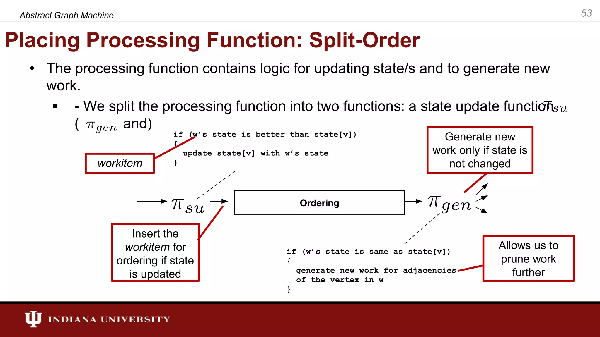
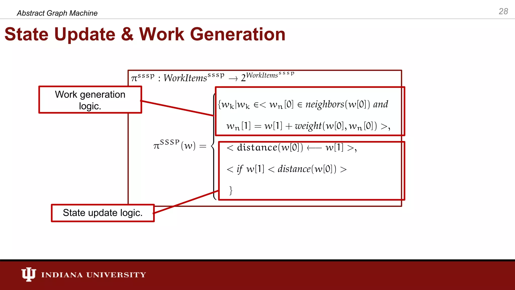
![The Processing Function for SSSP Input workitem. The workitem is a pair and w[0] returns the vertex associated to the workitem and w[1] returns the distance associated. 1. Check this condition. If input workitem’s distance is better than stored distance go to 2. 2. Updated distance and go to 3. 3. Generate new workitems. relax() in AGM notation 27Abstract Graph Machine](https://image.slidesharecdn.com/final-defense-thejaka-v2-181109144520/75/ABSTRACT-GRAPH-MACHINE-MODELING-ORDERINGS-IN-ASYNCHRONOUS-DISTRIBUTED-MEMORY-PARALLEL-GRAPH-ALGORITHMS-27-2048.jpg)
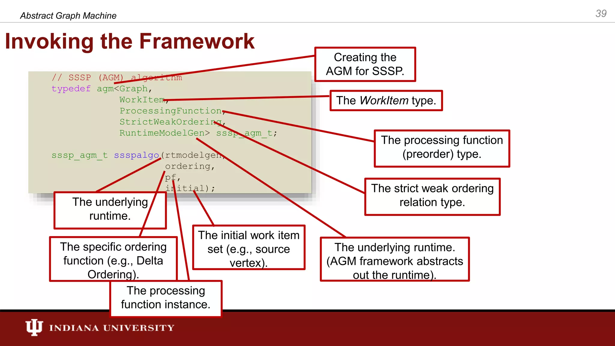
![template<typename buckets> void PF(const WorkItem& wi, int tid, buckets& outset) { Vertex v = std::get<0>(wi); Distance d = std::get<1>(wi); Distance old_dist = vdistance[v], last_old_dist; while (d < old_dist) { Distance din = CAS (d, &vdistance[v]); if (din == old_dist) { FORALL_OUTEDGES_T(v, e, g, Graph) { Vertex u = boost::target(e, g); Weight we = boost::get(vweight, e); WorkItem wigen(u, (d+we)); outset.push(wigen, tid); } break; } else { old_dist = din; } } } AGM Graph Processing Framework Abstract Graph Machine 38 //================== Dijkstra Ordering ===================== template<int index> struct dijkstra : public base_ordering { public: static const eagm_ordering ORDERING_NAME = eagm_ordering::enum_dijkstra; template <typename T> bool operator()(T i, T j) { return (std::get<index>(i) < std::get<index>(j)); } eagm_ordering name() { return ORDERING_NAME; } }; The strict weak ordering, partitions WorkItems. In this case the ordering is based on the distance. The processing function for SSSP. For SSSP a ”WorkItem” is a vertex and distance. CAS = Atomic compare & swap After executing wi, processing function generates new work items and they are pushed for ordering.](https://image.slidesharecdn.com/final-defense-thejaka-v2-181109144520/75/ABSTRACT-GRAPH-MACHINE-MODELING-ORDERINGS-IN-ASYNCHRONOUS-DISTRIBUTED-MEMORY-PARALLEL-GRAPH-ALGORITHMS-38-2048.jpg)