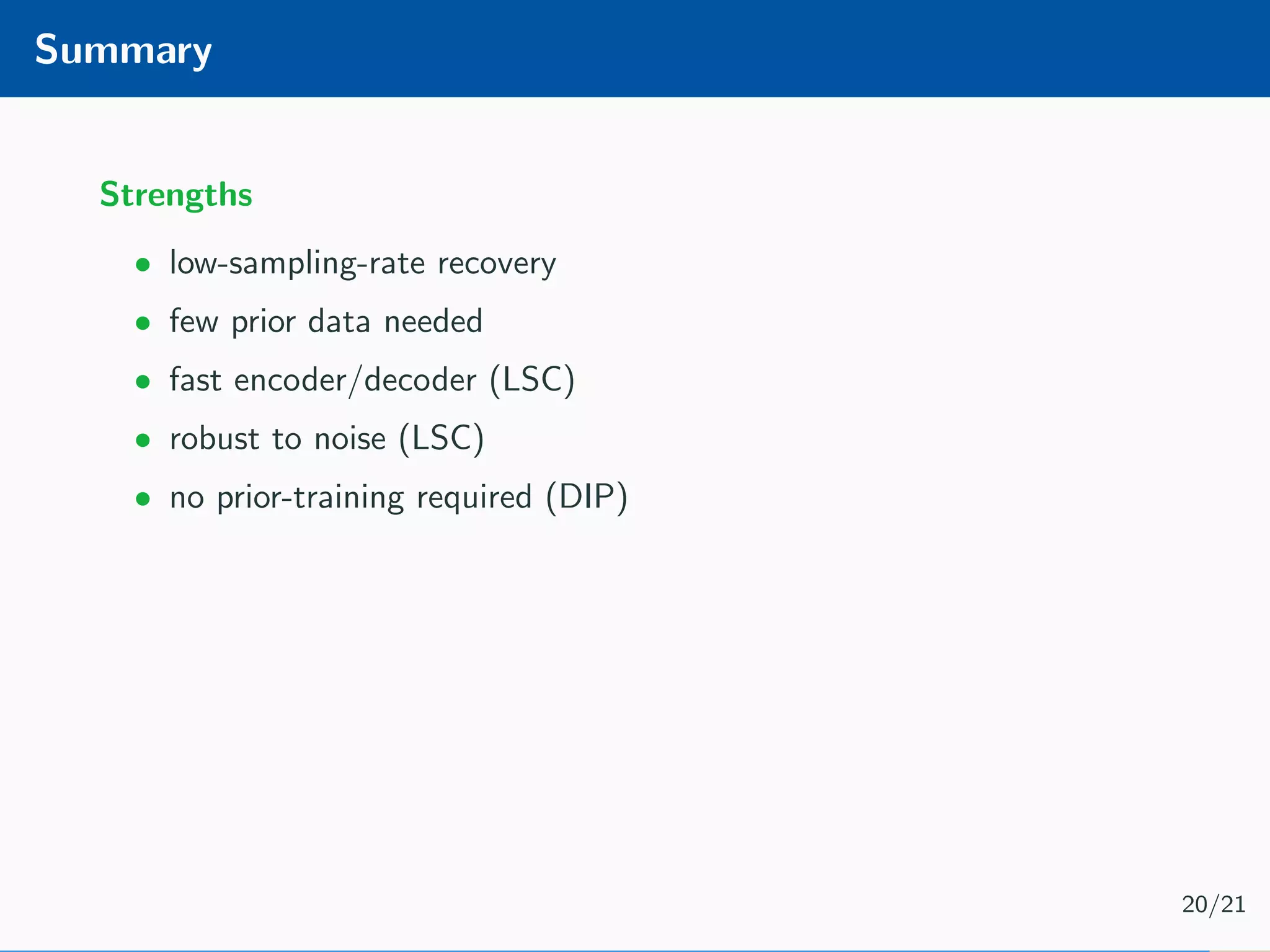
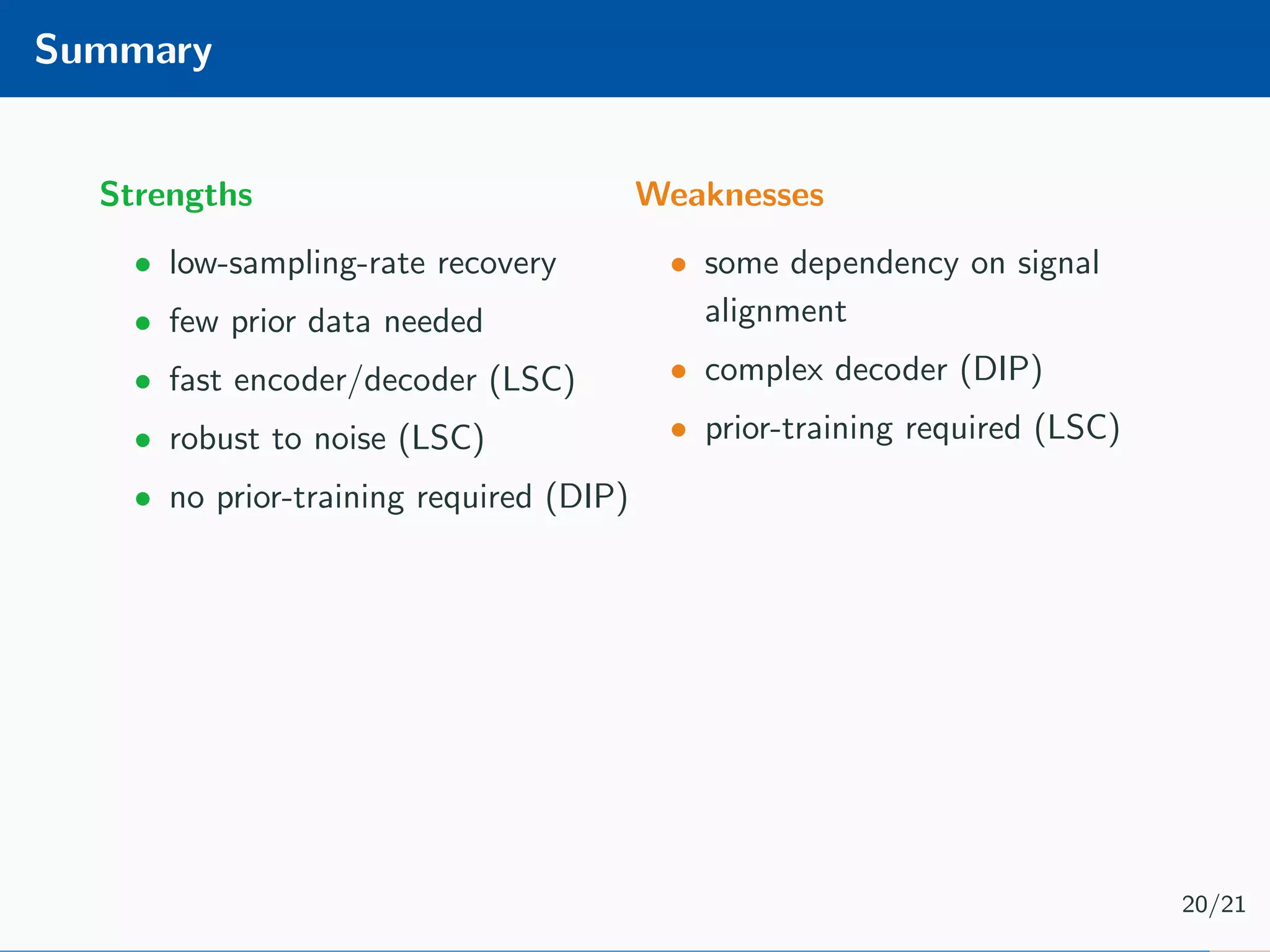
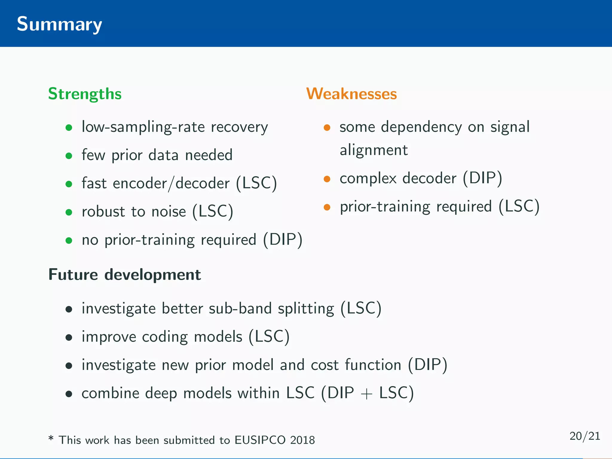
The document presents an approach to learnable compressive subsampling by integrating image priors, detailing methodologies, results, and applications. It highlights strengths such as low sampling rate recovery and robustness to noise, while noting weaknesses including dependency on signal alignment. Future development areas include improving coding models and investigating new prior models.
![CS Decoder The typical Compressive Subsampling decoding is performed by solving an optimisation problem, as for example the LASSO [1] minimisation: ˆx = arg min x Ax − b 2 2+α x 1 5/21](https://image.slidesharecdn.com/presentation-180922220836/75/Injecting-image-priors-into-Learnable-Compressive-Subsampling-14-2048.jpg)
![CS Decoder The typical Compressive Subsampling decoding is performed by solving an optimisation problem, as for example the LASSO [1] minimisation: ˆx = arg min x Ax − b 2 2+α x 1 Limitations: • computationally hard • noise over-fit 5/21](https://image.slidesharecdn.com/presentation-180922220836/75/Injecting-image-priors-into-Learnable-Compressive-Subsampling-15-2048.jpg)
![Learnable Compressive Subsampling Adaptive sampling (k-best) [2] Encoder Decoder Ψx × Ψ∗ ˆx learn Learnable CS (favg) [3] Encoder Decoder Ψx × Ψ∗ ˆx ΨX learn 7/21](https://image.slidesharecdn.com/presentation-180922220836/75/Injecting-image-priors-into-Learnable-Compressive-Subsampling-19-2048.jpg)
![Learnable Compressive Subsampling Adaptive sampling (k-best) [2] Encoder Decoder Ψx × Ψ∗ ˆx learn Encoder b = P ΩΨx Learnable CS (favg) [3] Encoder Decoder Ψx × Ψ∗ ˆx ΨX learn 7/21](https://image.slidesharecdn.com/presentation-180922220836/75/Injecting-image-priors-into-Learnable-Compressive-Subsampling-20-2048.jpg)
![Learnable Compressive Subsampling Adaptive sampling (k-best) [2] Encoder Decoder Ψx × Ψ∗ ˆx learn Encoder b = P ΩΨx Learnable CS (favg) [3] Encoder Decoder Ψx × Ψ∗ ˆx ΨX learn 7/21](https://image.slidesharecdn.com/presentation-180922220836/75/Injecting-image-priors-into-Learnable-Compressive-Subsampling-21-2048.jpg)
![Learnable Compressive Subsampling Adaptive sampling (k-best) [2] Encoder Decoder Ψx × Ψ∗ ˆx learn Encoder b = P ΩΨx Learnable CS (favg) [3] Encoder Decoder Ψx × Ψ∗ ˆx ΨX learn Decoder ˆx = Ψ∗ P T Ωb 7/21](https://image.slidesharecdn.com/presentation-180922220836/75/Injecting-image-priors-into-Learnable-Compressive-Subsampling-22-2048.jpg)
![Learnable Compressive Subsampling Adaptive sampling (k-best) [2] Encoder Decoder Ψx × Ψ∗ ˆx learn Encoder b = P ΩΨx Learnable CS (favg) [3] Encoder Decoder Ψx × Ψ∗ ˆx ΨX learn Decoder ˆx = Ψ∗ P T Ωb Learning ˆΩ = arg max Ω P ΩΨx 2 2 Learning ˆΩ = arg max Ω N i=1 P ΩΨxi 2 2 7/21](https://image.slidesharecdn.com/presentation-180922220836/75/Injecting-image-priors-into-Learnable-Compressive-Subsampling-23-2048.jpg)


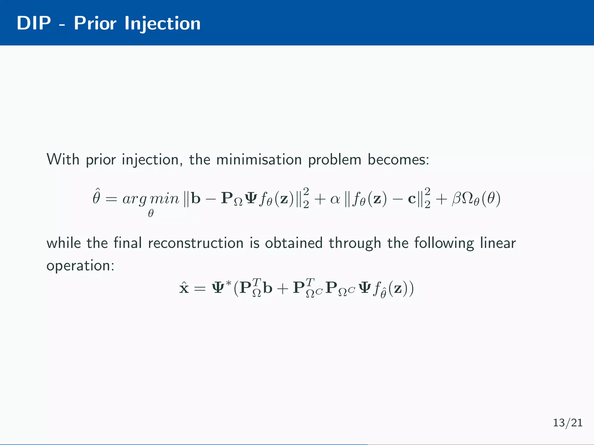
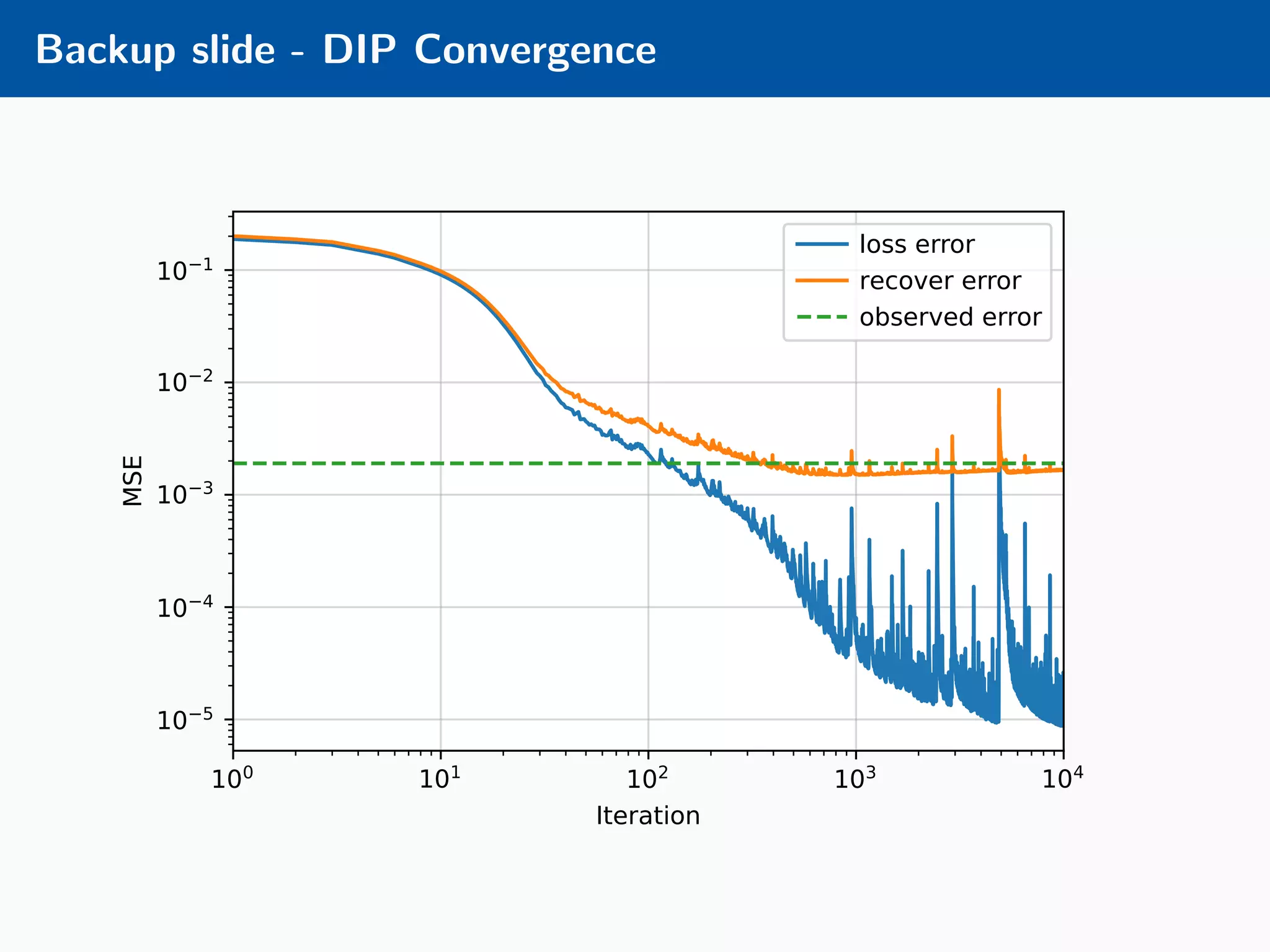
![DIP - Overview Implement a hourglass network [4] using the Deep Image Prior [5] framework: Minimisation problem is as follow: ˆθ = arg min θ b − PΩΨfθ(z) 2 2 + βΩθ(θ) 12/21](https://image.slidesharecdn.com/presentation-180922220836/75/Injecting-image-priors-into-Learnable-Compressive-Subsampling-36-2048.jpg)