Download as PDF, PPTX


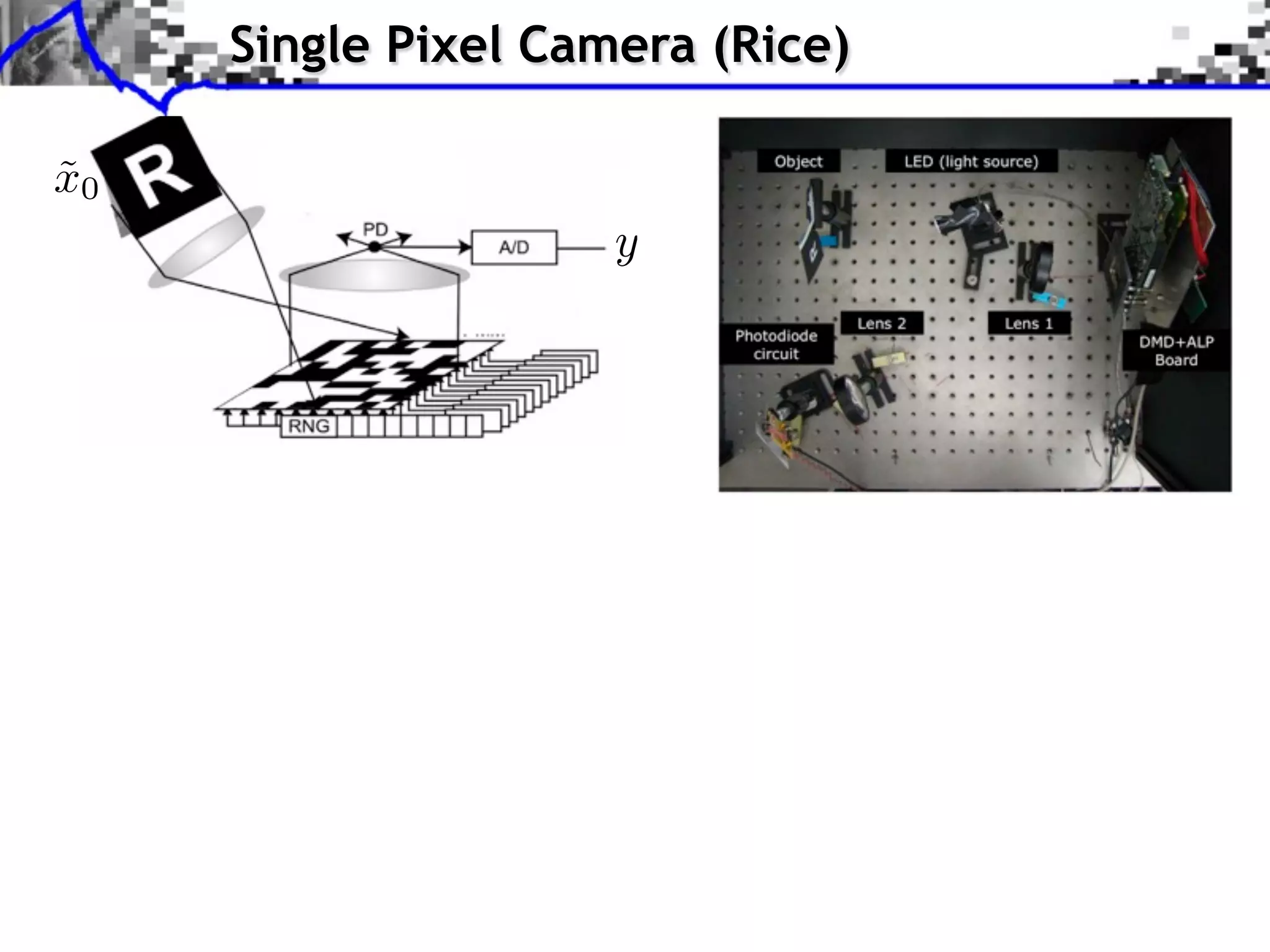
![Single Pixel Camera (Rice) x0 ˜ y[i] = hx0 , 'i i P measures N micro-mirrors](https://image.slidesharecdn.com/2013-11-29-astro-131129111249-phpapp02/75/Low-Complexity-Regularization-of-Inverse-Problems-4-2048.jpg)
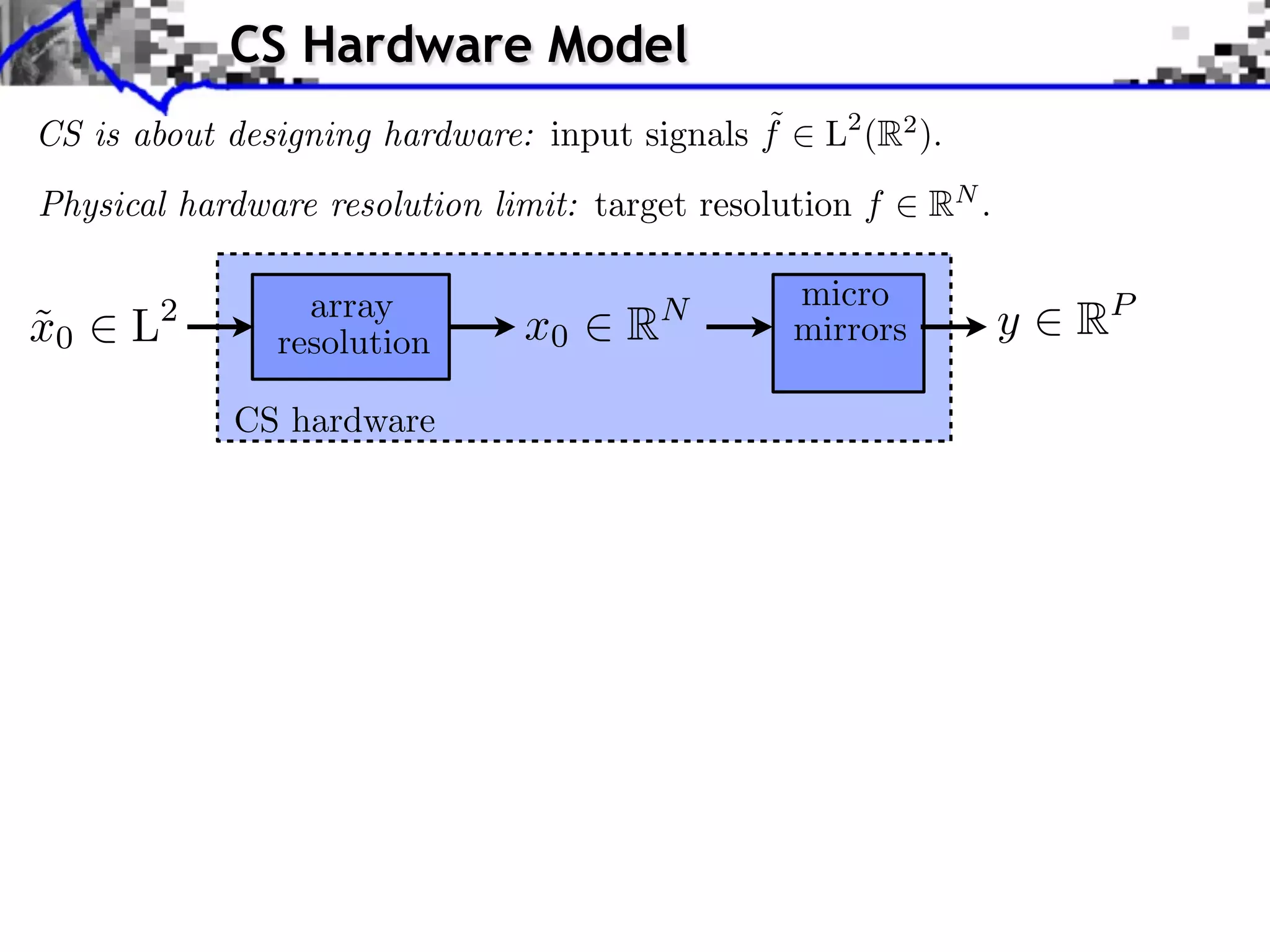
![Single Pixel Camera (Rice) x0 ˜ y[i] = hx0 , 'i i P measures P/N = 1 N micro-mirrors P/N = 0.16 P/N = 0.02](https://image.slidesharecdn.com/2013-11-29-astro-131129111249-phpapp02/75/Low-Complexity-Regularization-of-Inverse-Problems-5-2048.jpg)
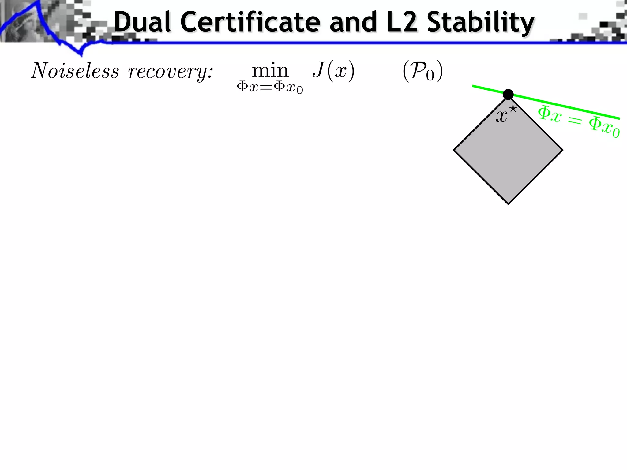
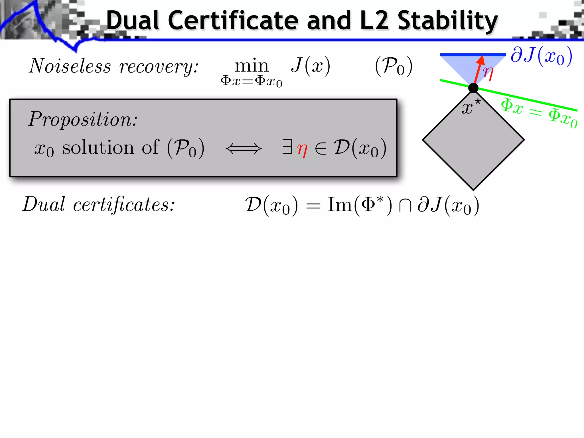
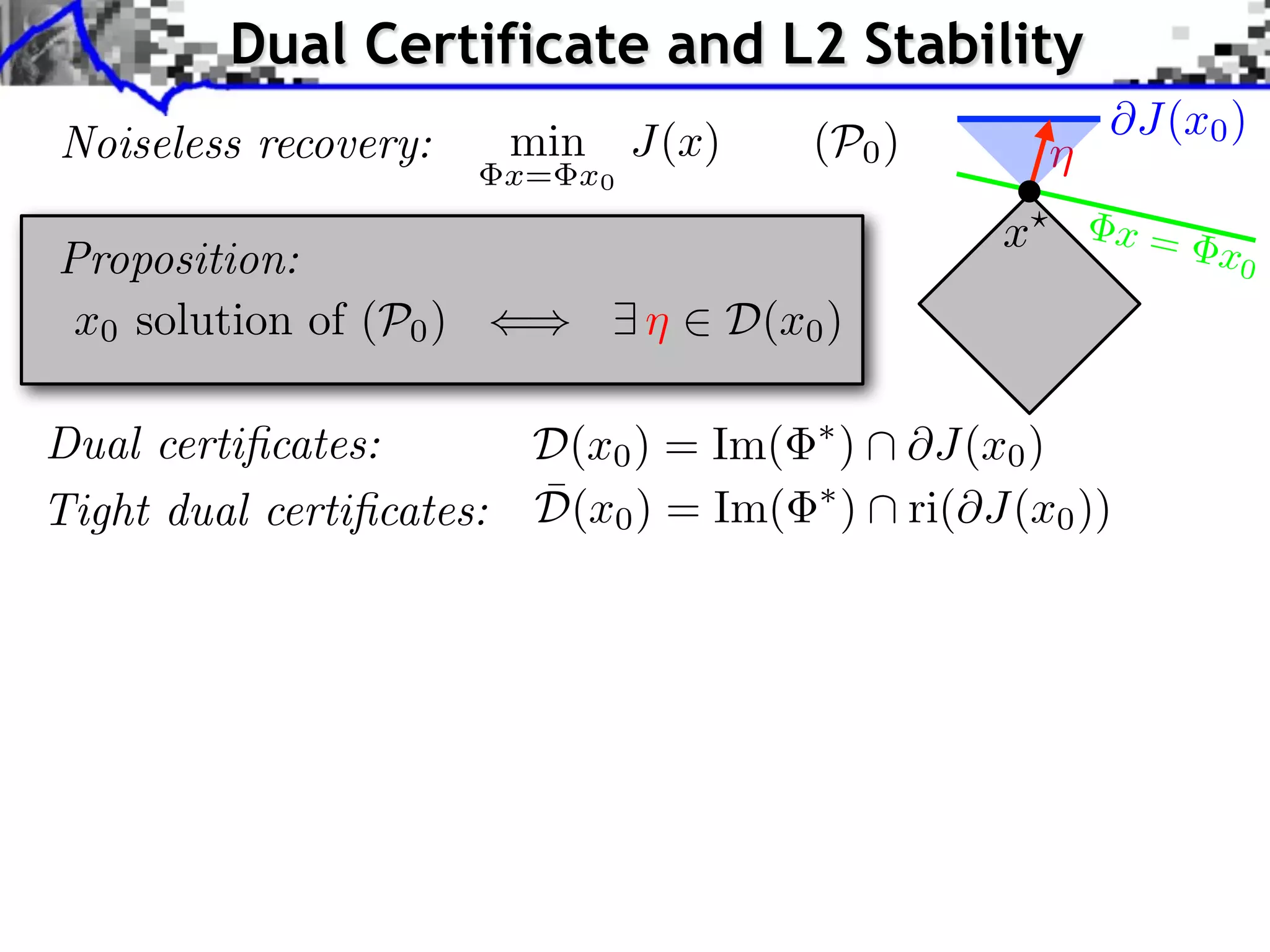
![Dual Certificate and L2 Stability Noiseless recovery: min J(x) x= x0 (P0 ) Proposition: x0 solution of (P0 ) () 9 ⌘ 2 D(x0 ) Dual certificates: D(x0 ) = Im( ¯ Tight dual certificates: D(x0 ) = Im( Theorem: ¯ If 9 ⌘ 2 D(x0 ), for ⌘ @J(x0 ) x? x= x0 ⇤ ) @J(x0 ) ⇤ ) ri(@J(x0 )) [Fadili et al. 2013] ⇠ ||w|| one has ||x? x0 || = O(||w||)](https://image.slidesharecdn.com/2013-11-29-astro-131129111249-phpapp02/75/Low-Complexity-Regularization-of-Inverse-Problems-36-2048.jpg)
![Dual Certificate and L2 Stability Noiseless recovery: min J(x) x= x0 (P0 ) Proposition: x0 solution of (P0 ) () 9 ⌘ 2 D(x0 ) Dual certificates: D(x0 ) = Im( ¯ Tight dual certificates: D(x0 ) = Im( Theorem: ¯ If 9 ⌘ 2 D(x0 ), for ⌘ @J(x0 ) x? x= x0 ⇤ ) @J(x0 ) ⇤ ) ri(@J(x0 )) [Fadili et al. 2013] ⇠ ||w|| one has ||x? x0 || = O(||w||) [Grassmair, Haltmeier, Scherzer 2010]: J = || · ||1 . [Grassmair 2012]: J(x? x0 ) = O(||w||).](https://image.slidesharecdn.com/2013-11-29-astro-131129111249-phpapp02/75/Low-Complexity-Regularization-of-Inverse-Problems-37-2048.jpg)
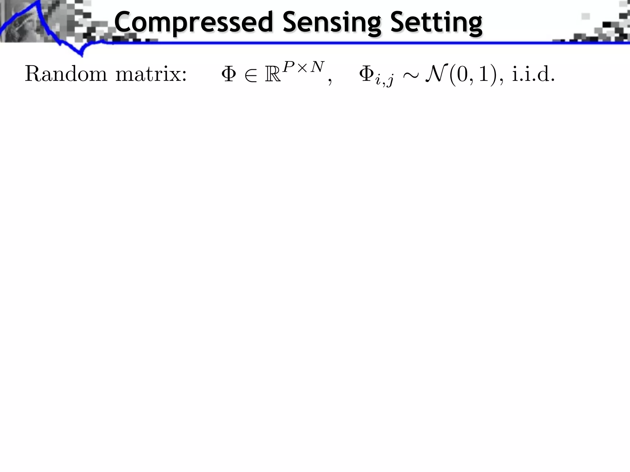
![Compressed Sensing Setting Random matrix: 2 RP ⇥N , Sparse vectors: J = || · ||1 . Theorem: Let s = ||x0 ||0 . If i,j ⇠ N (0, 1), i.i.d. [Rudelson, Vershynin 2006] [Chandrasekaran et al. 2011] P > 2s log (N/s) ¯ Then 9⌘ 2 D(x0 ) with high probability on .](https://image.slidesharecdn.com/2013-11-29-astro-131129111249-phpapp02/75/Low-Complexity-Regularization-of-Inverse-Problems-39-2048.jpg)
![Compressed Sensing Setting Random matrix: 2 RP ⇥N , Sparse vectors: J = || · ||1 . Theorem: Let s = ||x0 ||0 . If i,j ⇠ N (0, 1), i.i.d. [Rudelson, Vershynin 2006] [Chandrasekaran et al. 2011] P > 2s log (N/s) ¯ Then 9⌘ 2 D(x0 ) with high probability on Low-rank matrices: J = || · ||⇤ . Theorem: Let r = rank(x0 ). If . [Chandrasekaran et al. 2011] x0 2 RN1 ⇥N2 P > 3r(N1 + N2 r) ¯ Then 9⌘ 2 D(x0 ) with high probability on .](https://image.slidesharecdn.com/2013-11-29-astro-131129111249-phpapp02/75/Low-Complexity-Regularization-of-Inverse-Problems-40-2048.jpg)
![Compressed Sensing Setting Random matrix: 2 RP ⇥N , Sparse vectors: J = || · ||1 . Theorem: Let s = ||x0 ||0 . If i,j ⇠ N (0, 1), i.i.d. [Rudelson, Vershynin 2006] [Chandrasekaran et al. 2011] P > 2s log (N/s) ¯ Then 9⌘ 2 D(x0 ) with high probability on Low-rank matrices: J = || · ||⇤ . Theorem: Let r = rank(x0 ). If . [Chandrasekaran et al. 2011] x0 2 RN1 ⇥N2 P > 3r(N1 + N2 r) ¯ Then 9⌘ 2 D(x0 ) with high probability on ! Similar results for || · ||1,2 , || · ||1 . .](https://image.slidesharecdn.com/2013-11-29-astro-131129111249-phpapp02/75/Low-Complexity-Regularization-of-Inverse-Problems-41-2048.jpg)
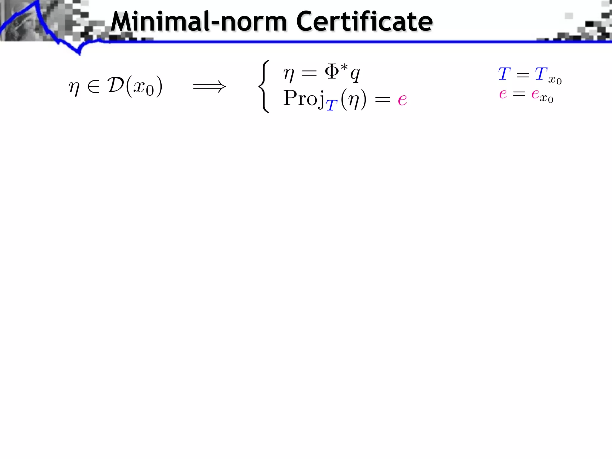
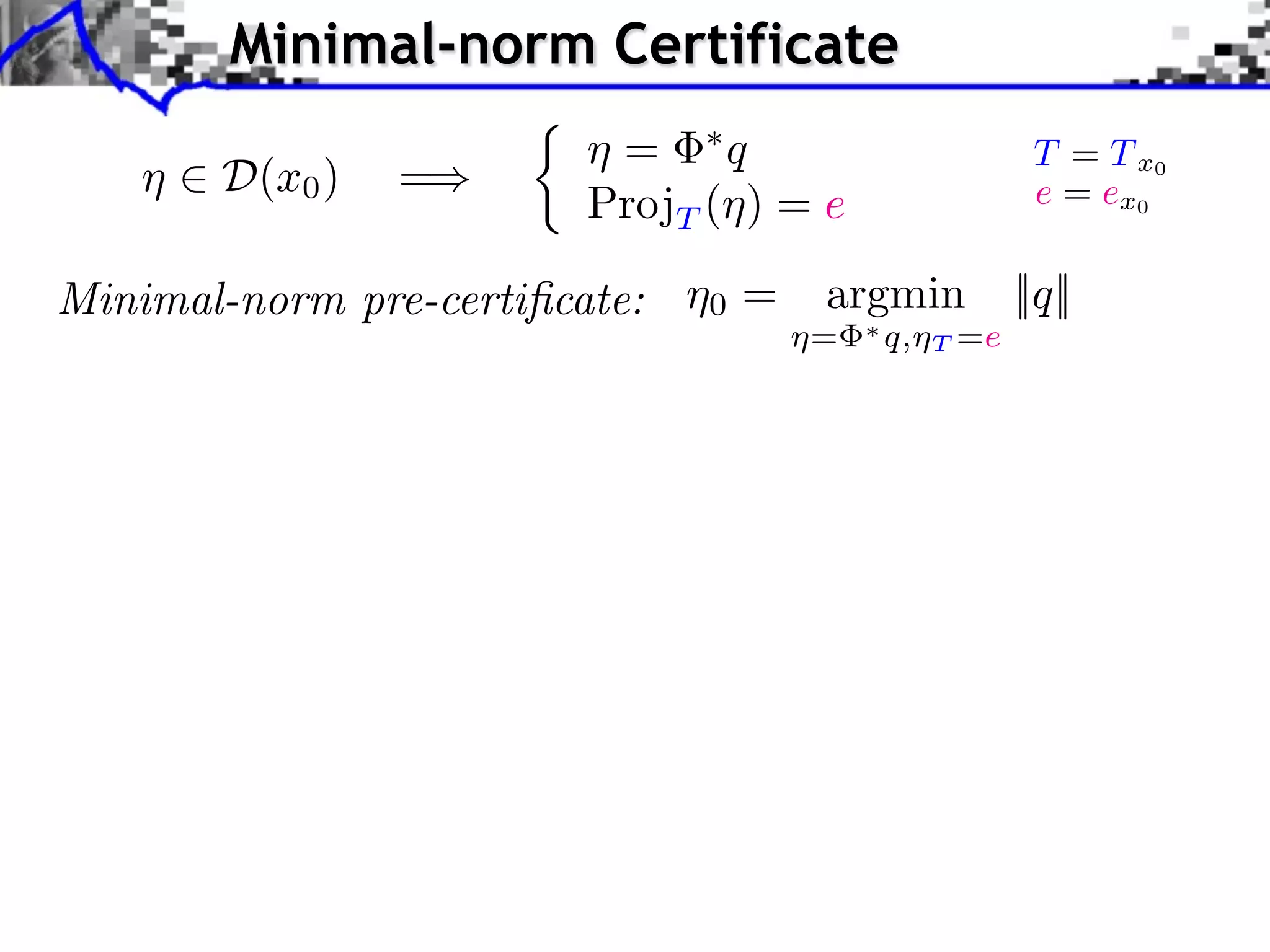
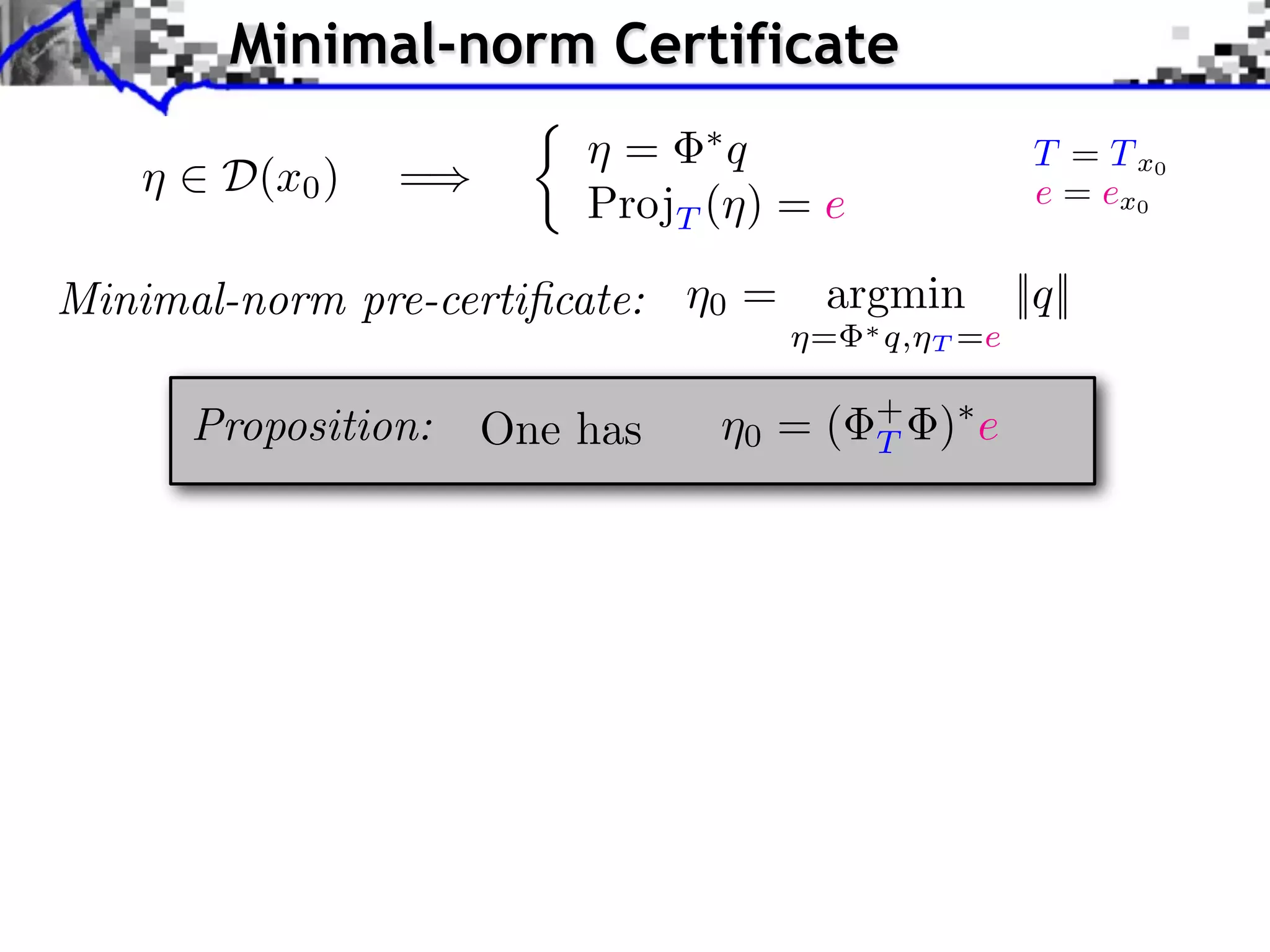
![Minimal-norm Certificate ⌘ 2 D(x0 ) =) ⇢ ⌘ = ⇤q ProjT (⌘) = e Minimal-norm pre-certificate: ⌘0 = argmin ⌘= One has ⌘0 = ( ¯ If ⌘0 2 D(x0 ) and ⇤ q,⌘ + T T =e ||q|| )⇤ e ⇠ ||w||, Proposition: Theorem: T = T x0 e = ex0 the unique solution x? of P (y) for y = x0 + w satisfies Tx ? = T x 0 and ||x? x0 || = O(||w||) [Vaiter et al. 2013]](https://image.slidesharecdn.com/2013-11-29-astro-131129111249-phpapp02/75/Low-Complexity-Regularization-of-Inverse-Problems-45-2048.jpg)
![Minimal-norm Certificate ⌘ 2 D(x0 ) =) ⇢ ⌘ = ⇤q ProjT (⌘) = e Minimal-norm pre-certificate: ⌘0 = argmin ⌘= One has ⌘0 = ( ¯ If ⌘0 2 D(x0 ) and ⇤ q,⌘ + T T =e ||q|| )⇤ e ⇠ ||w||, Proposition: Theorem: T = T x0 e = ex0 the unique solution x? of P (y) for y = x0 + w satisfies Tx ? = T x 0 and ||x? x0 || = O(||w||) [Vaiter et al. 2013] [Fuchs 2004]: J = || · ||1 . [Vaiter et al. 2011]: J = ||D⇤ · ||1 . [Bach 2008]: J = || · ||1,2 and J = || · ||⇤ .](https://image.slidesharecdn.com/2013-11-29-astro-131129111249-phpapp02/75/Low-Complexity-Regularization-of-Inverse-Problems-46-2048.jpg)
![Compressed Sensing Setting Random matrix: 2 RP ⇥N , Sparse vectors: J = || · ||1 . Theorem: Let s = ||x0 ||0 . If i,j ⇠ N (0, 1), i.i.d. [Wainwright 2009] [Dossal et al. 2011] P > 2s log(N ) ¯ Then ⌘0 2 D( x0 ) wi th hi g h prob a b i l i ty on .](https://image.slidesharecdn.com/2013-11-29-astro-131129111249-phpapp02/75/Low-Complexity-Regularization-of-Inverse-Problems-47-2048.jpg)
![Compressed Sensing Setting Random matrix: 2 RP ⇥N , i,j Sparse vectors: J = || · ||1 . ⇠ N (0, 1), i.i.d. [Wainwright 2009] [Dossal et al. 2011] Theorem: Let s = ||x0 ||0 . If P > 2s log(N ) ¯ Then ⌘0 2 D( x0 ) wi th hi g h prob a b i l i ty on Phase transitions: L2 stability P ⇠ 2s log(N/s) vs. . Model stability P ⇠ 2s log(N )](https://image.slidesharecdn.com/2013-11-29-astro-131129111249-phpapp02/75/Low-Complexity-Regularization-of-Inverse-Problems-48-2048.jpg)
![Compressed Sensing Setting Random matrix: 2 RP ⇥N , i,j Sparse vectors: J = || · ||1 . ⇠ N (0, 1), i.i.d. [Wainwright 2009] [Dossal et al. 2011] Theorem: Let s = ||x0 ||0 . If P > 2s log(N ) ¯ Then ⌘0 2 D( x0 ) wi th hi g h prob a b i l i ty on Phase transitions: L2 stability P ⇠ 2s log(N/s) vs. . Model stability ! Similar results for || · ||1,2 , || · ||⇤ , || · ||1 . P ⇠ 2s log(N )](https://image.slidesharecdn.com/2013-11-29-astro-131129111249-phpapp02/75/Low-Complexity-Regularization-of-Inverse-Problems-49-2048.jpg)
![Compressed Sensing Setting Random matrix: 2 RP ⇥N , i,j Sparse vectors: J = || · ||1 . ⇠ N (0, 1), i.i.d. [Wainwright 2009] [Dossal et al. 2011] Theorem: Let s = ||x0 ||0 . If P > 2s log(N ) ¯ Then ⌘0 2 D( x0 ) wi th hi g h prob a b i l i ty on Phase transitions: L2 stability P ⇠ 2s log(N/s) vs. . Model stability ! Similar results for || · ||1,2 , || · ||⇤ , || · ||1 . P ⇠ 2s log(N ) ! Not using RIP technics (non-uniform result on x0 ).](https://image.slidesharecdn.com/2013-11-29-astro-131129111249-phpapp02/75/Low-Complexity-Regularization-of-Inverse-Problems-50-2048.jpg)
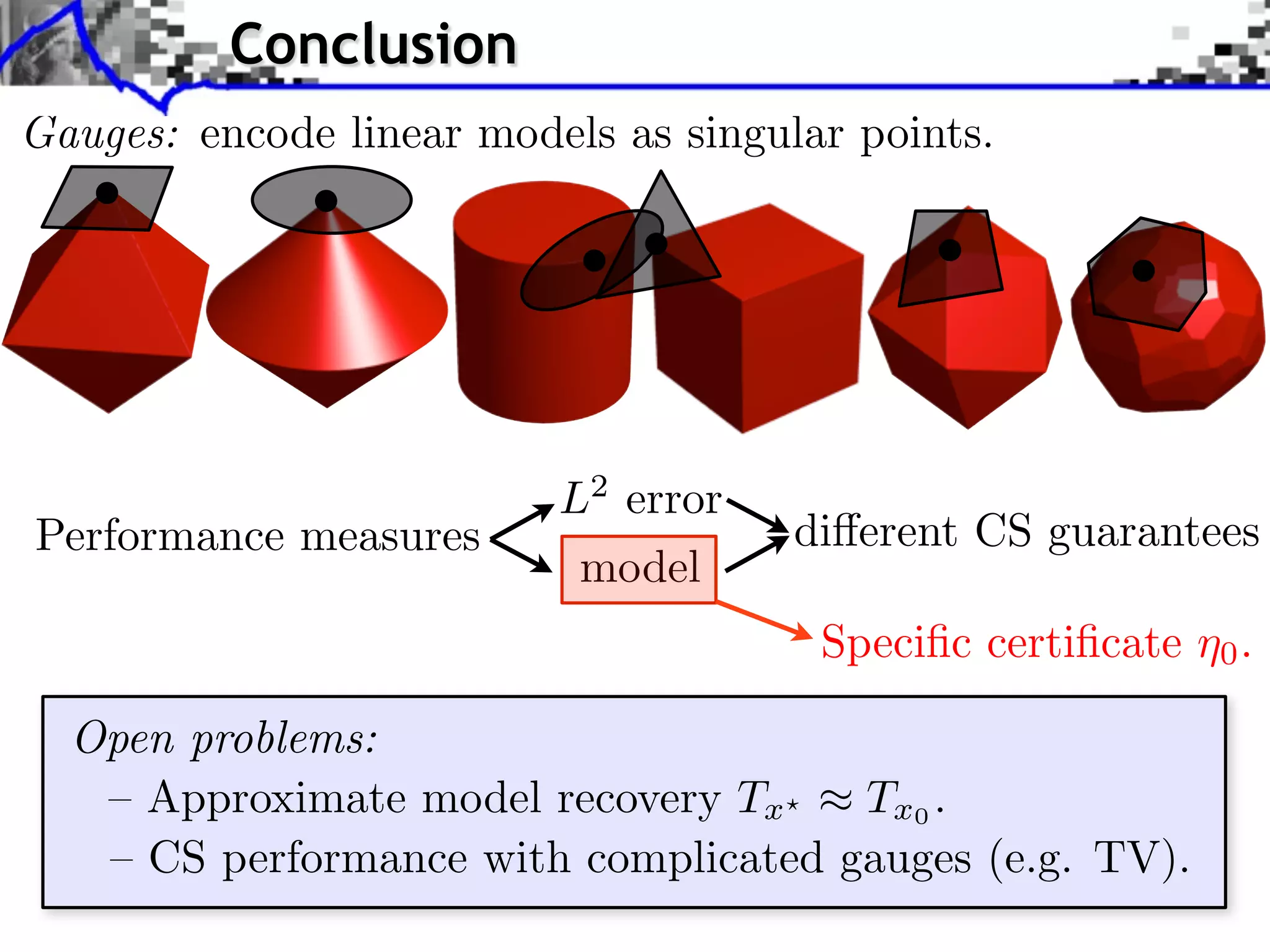

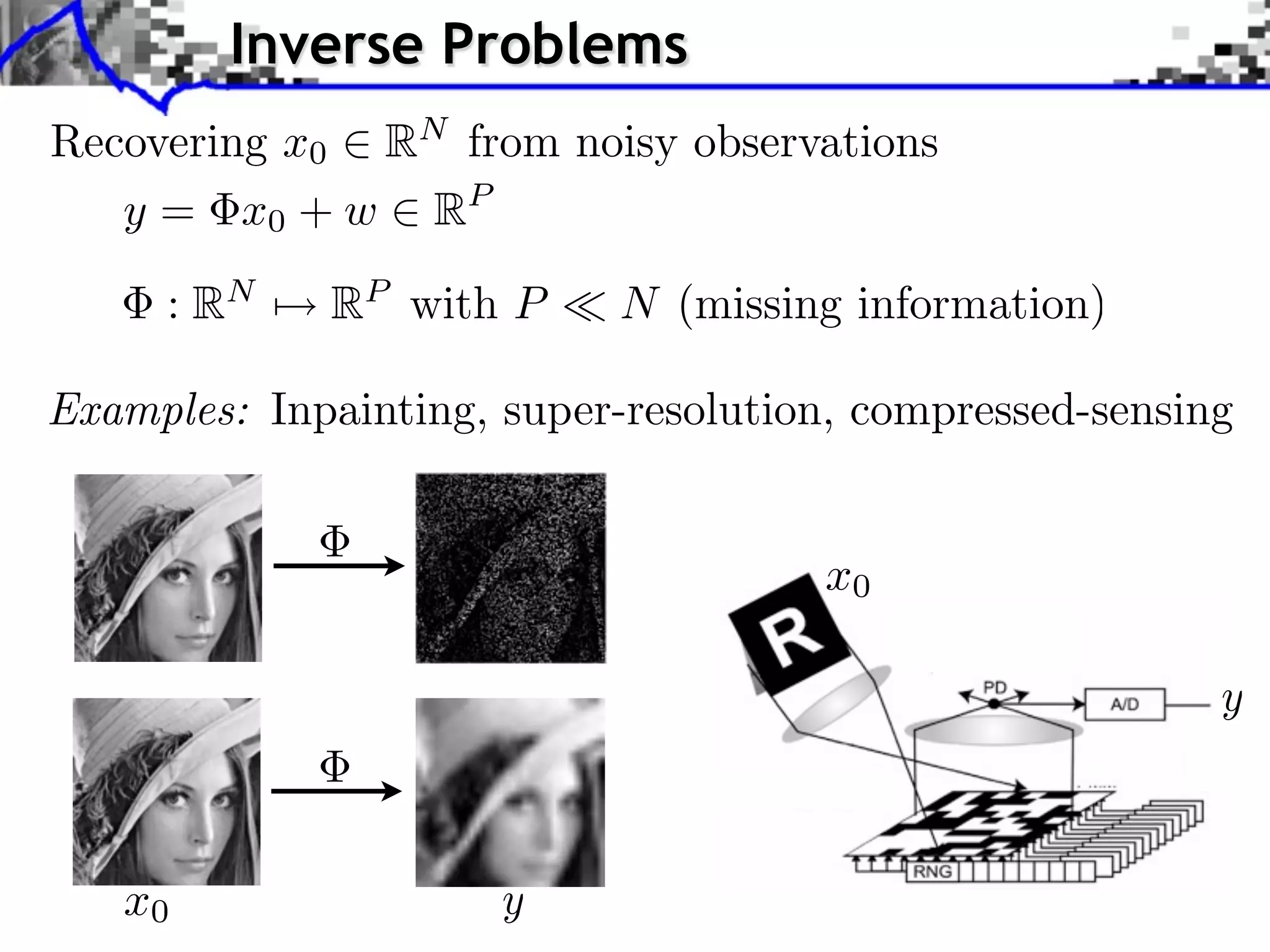
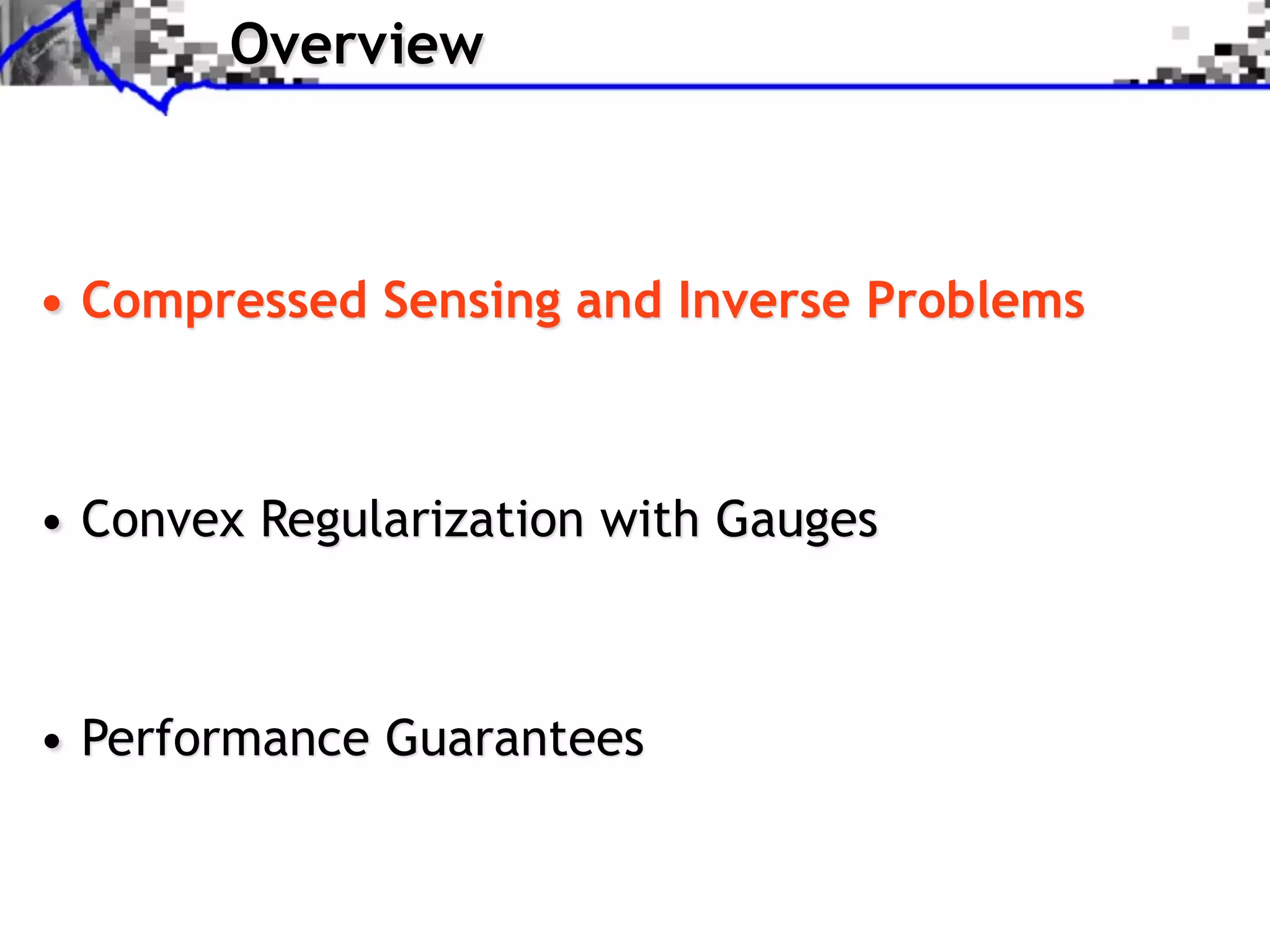
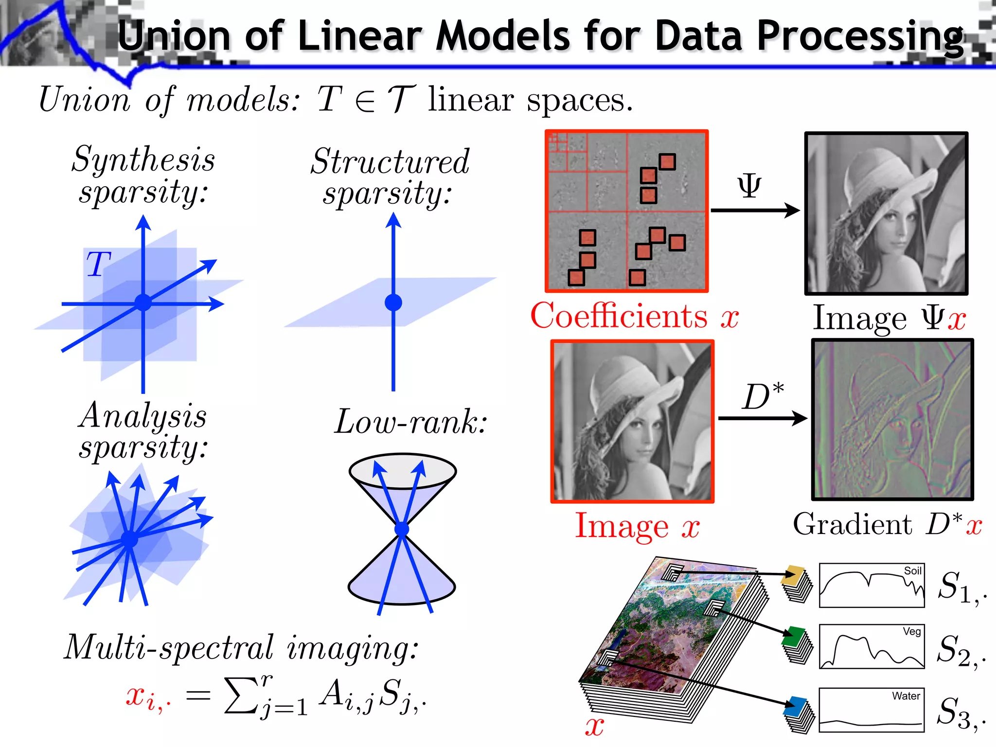
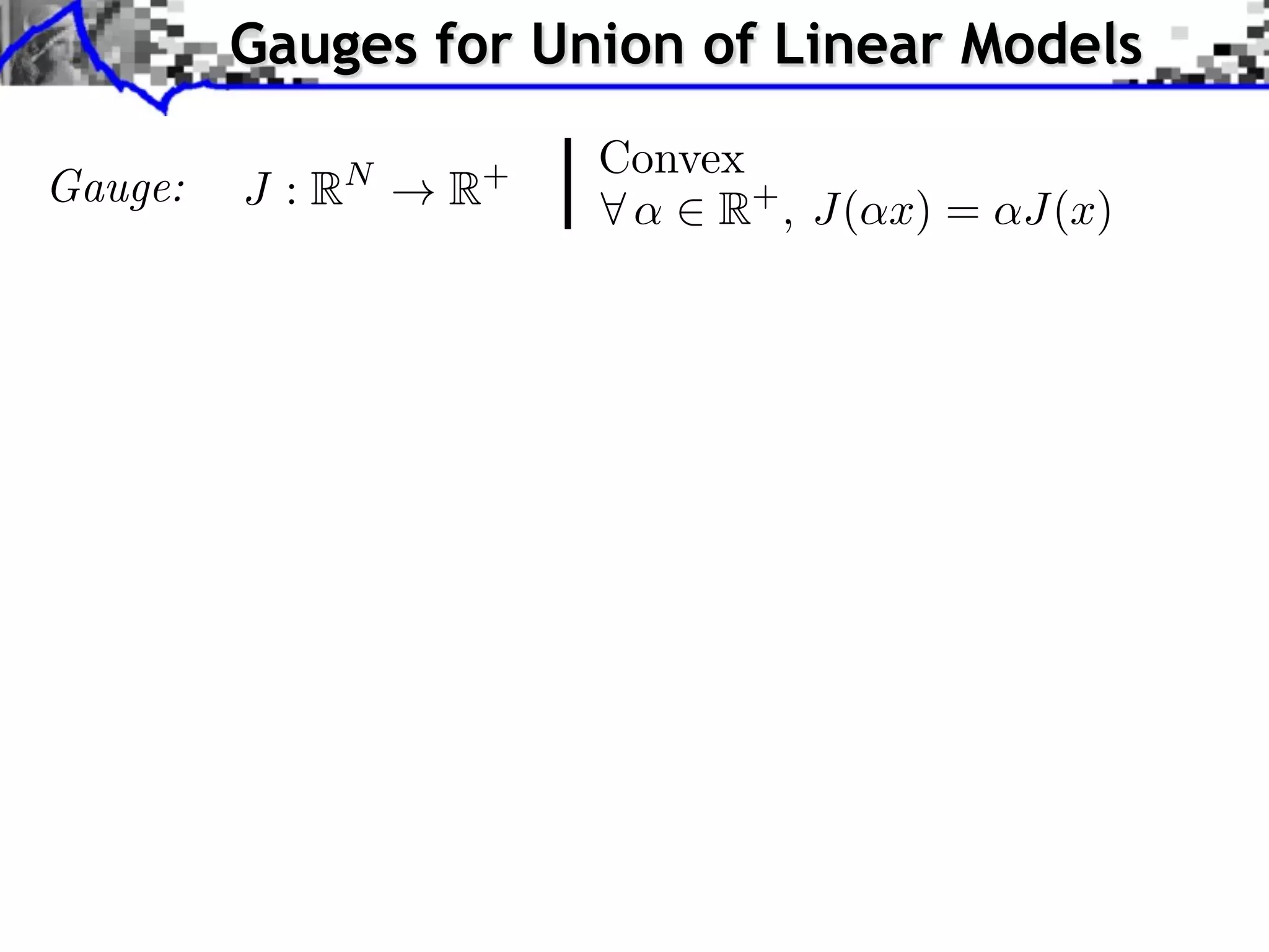
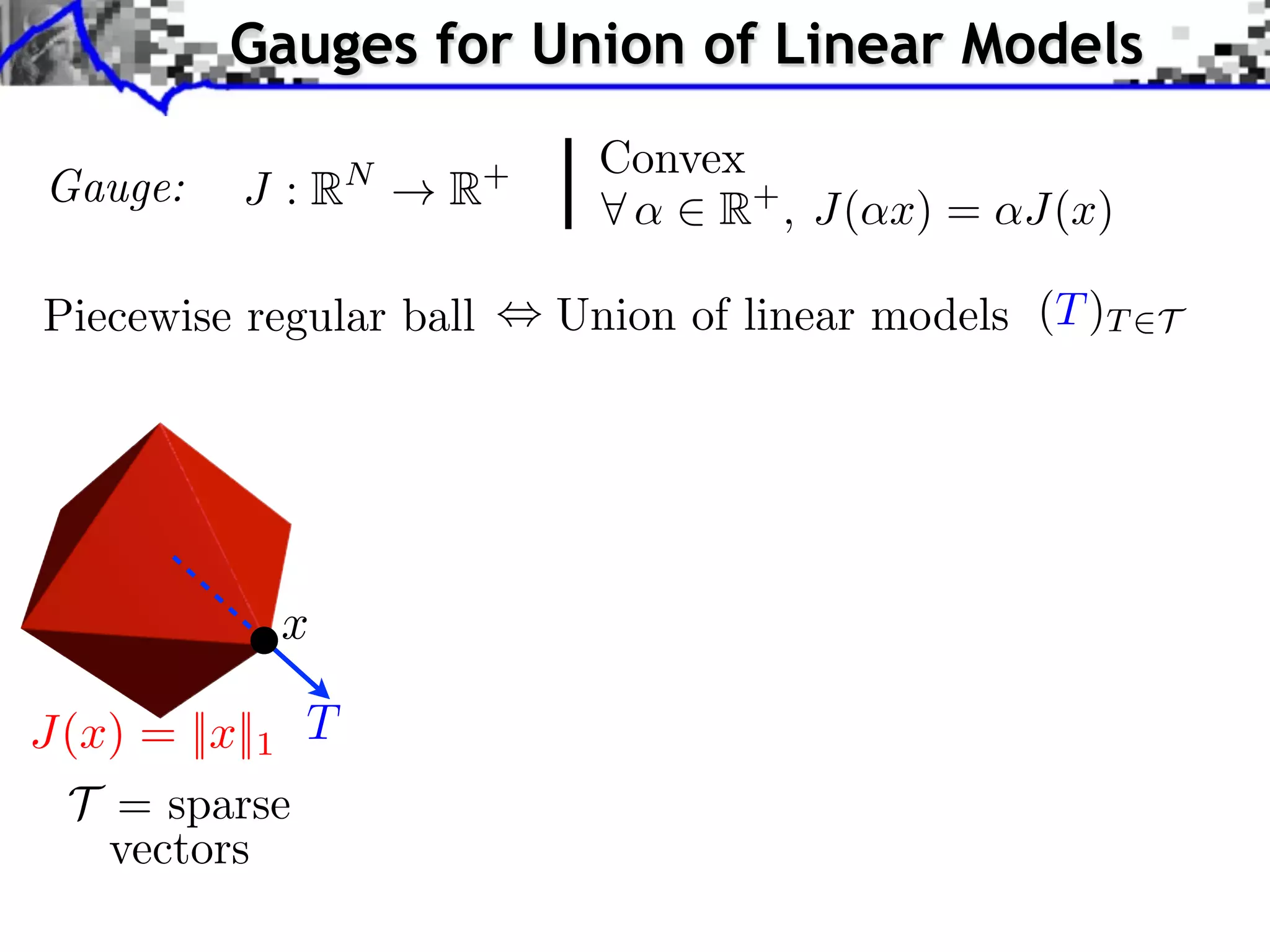
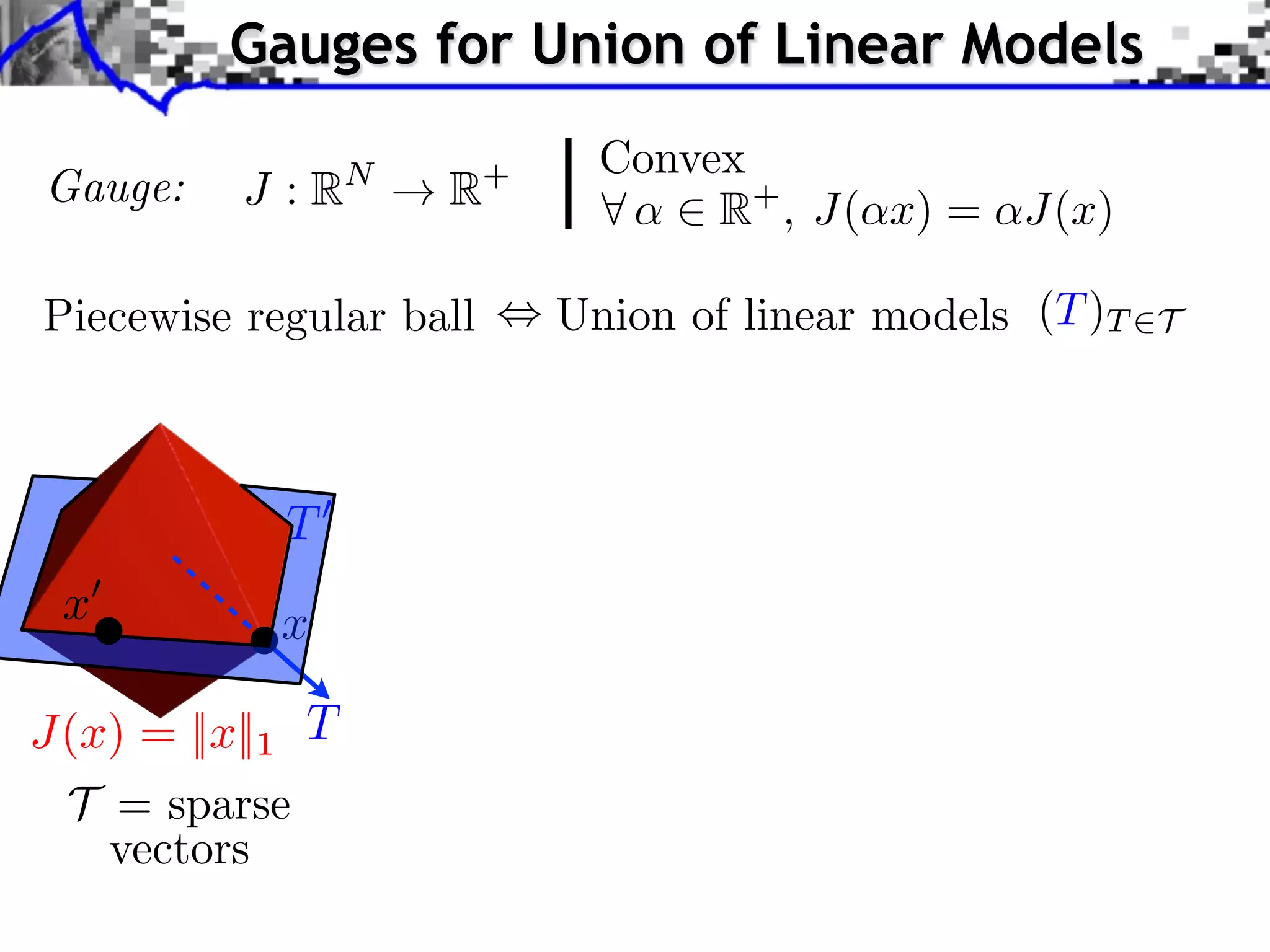
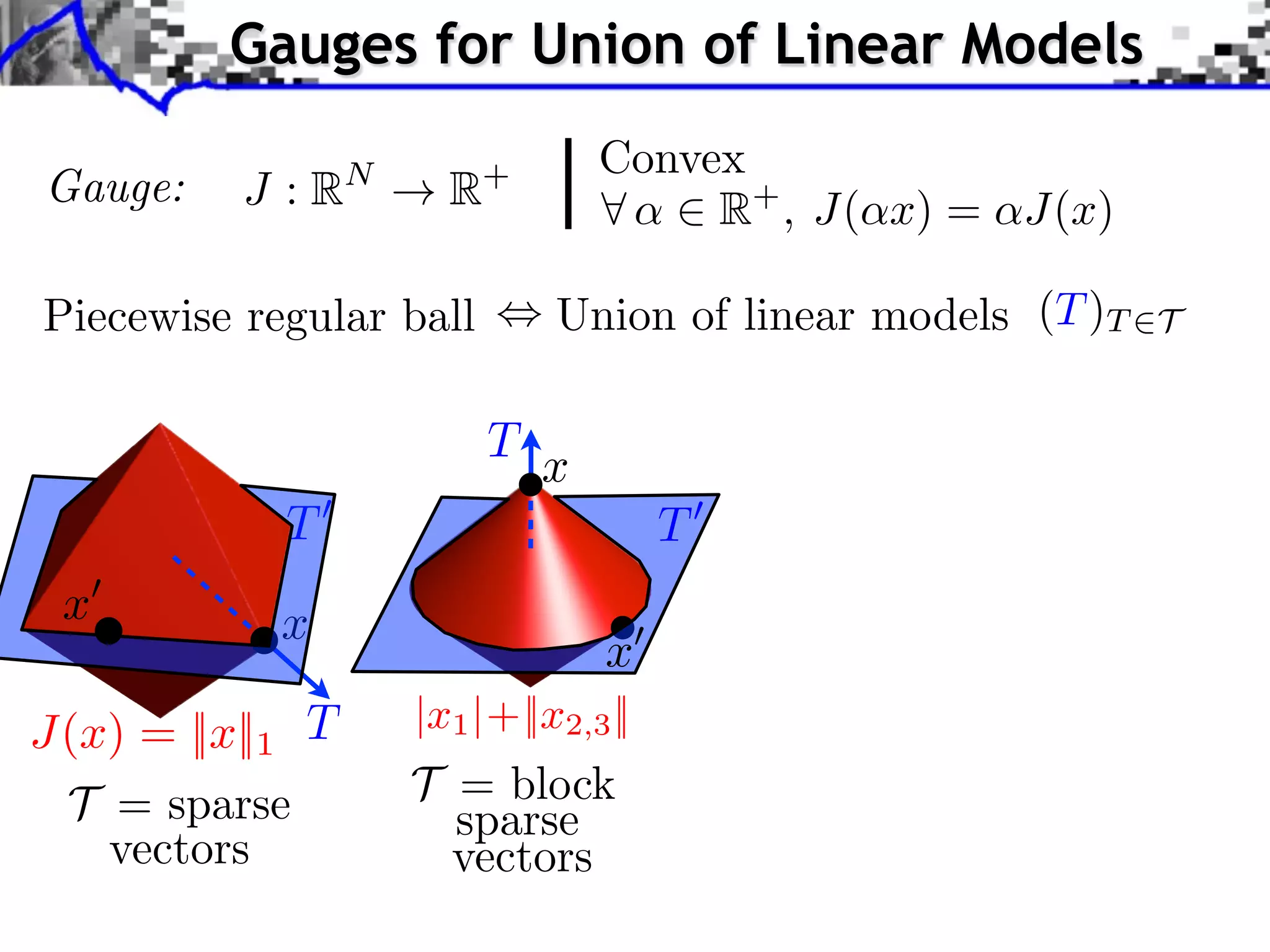
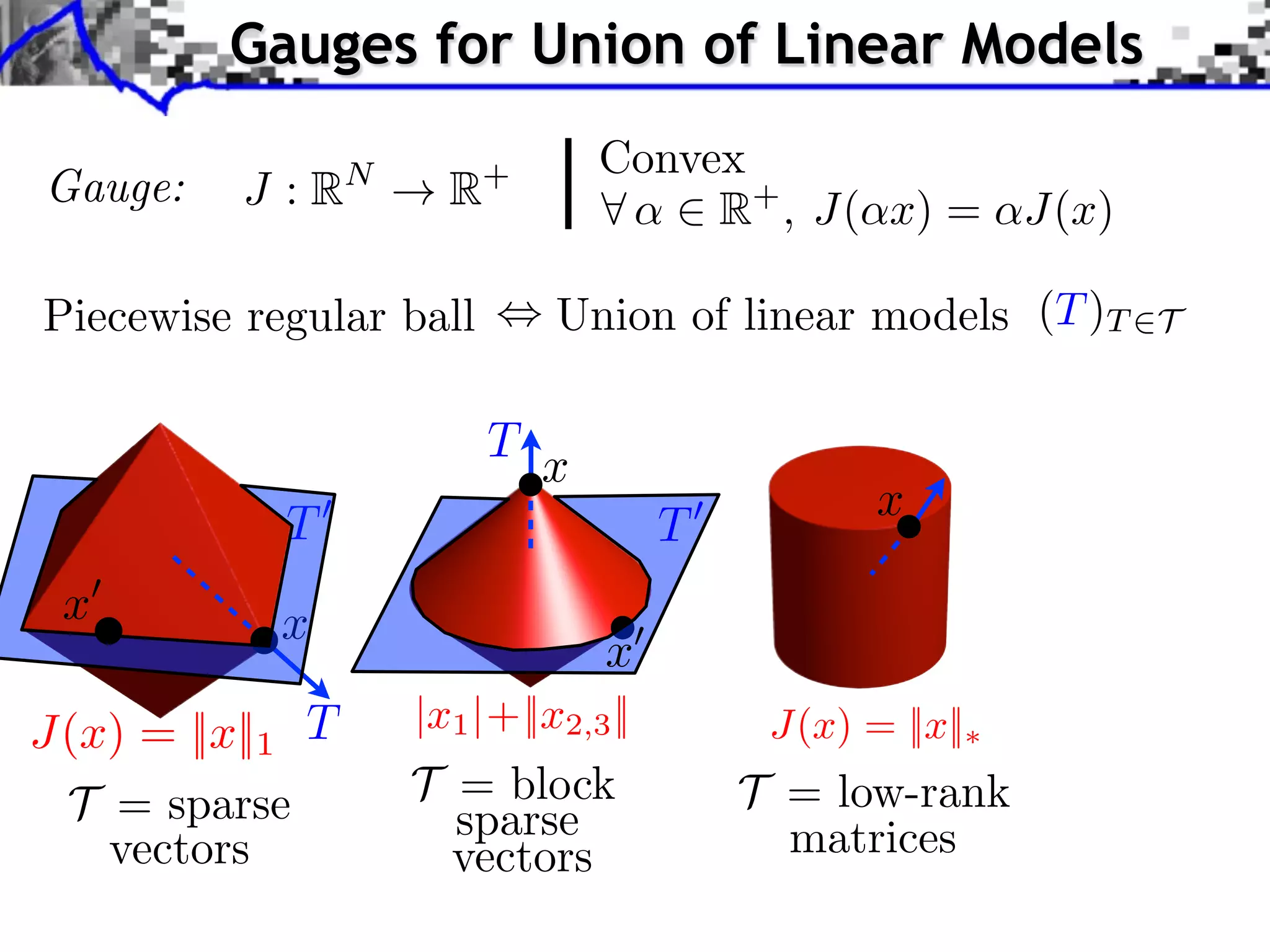
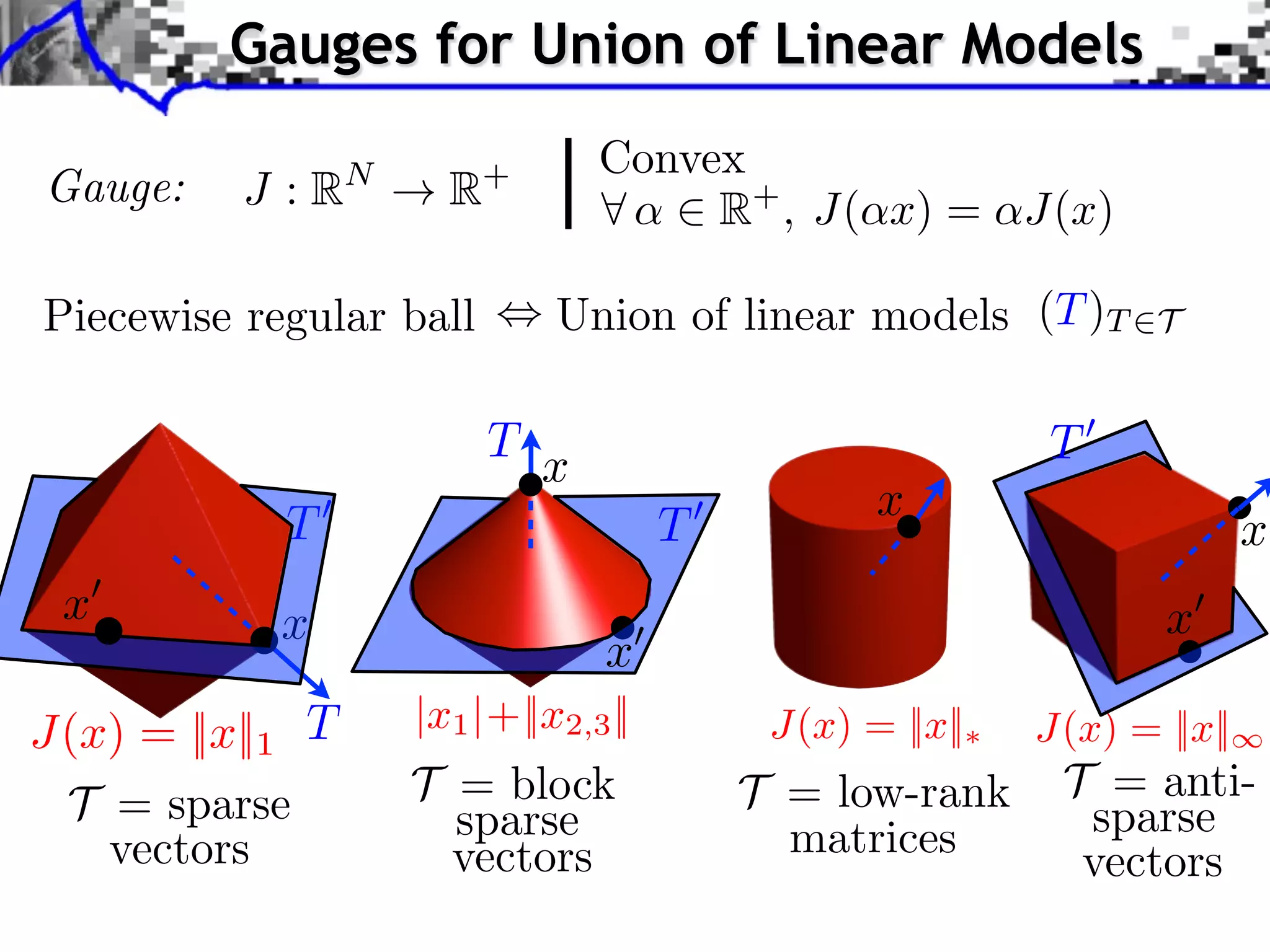
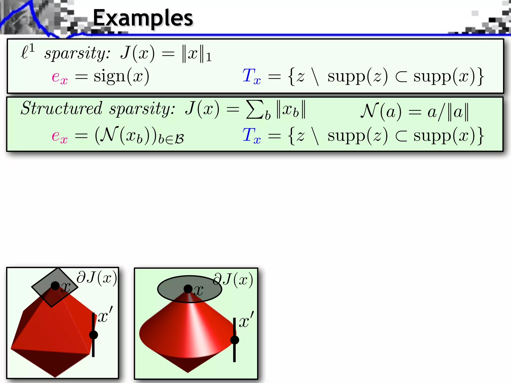
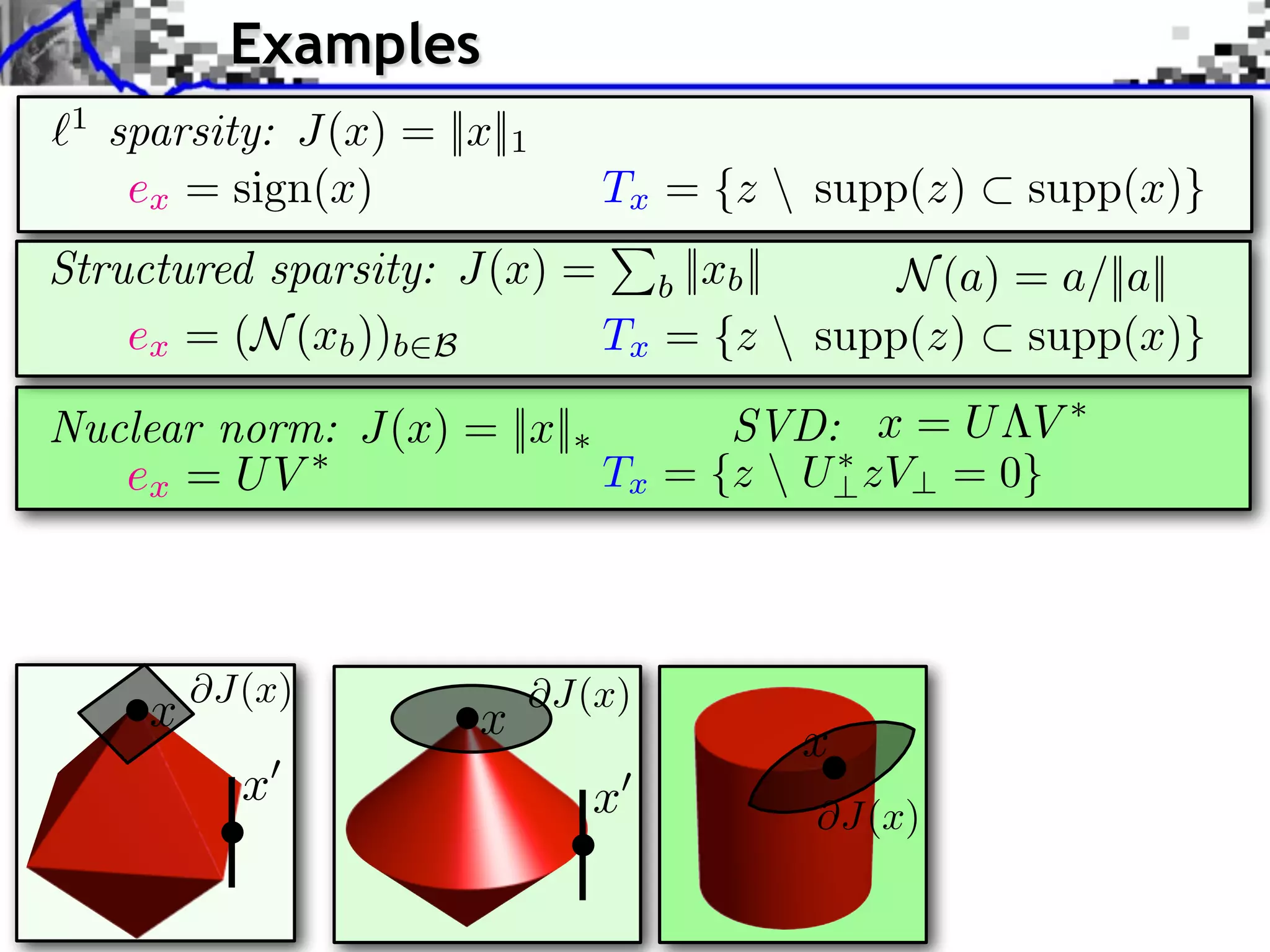
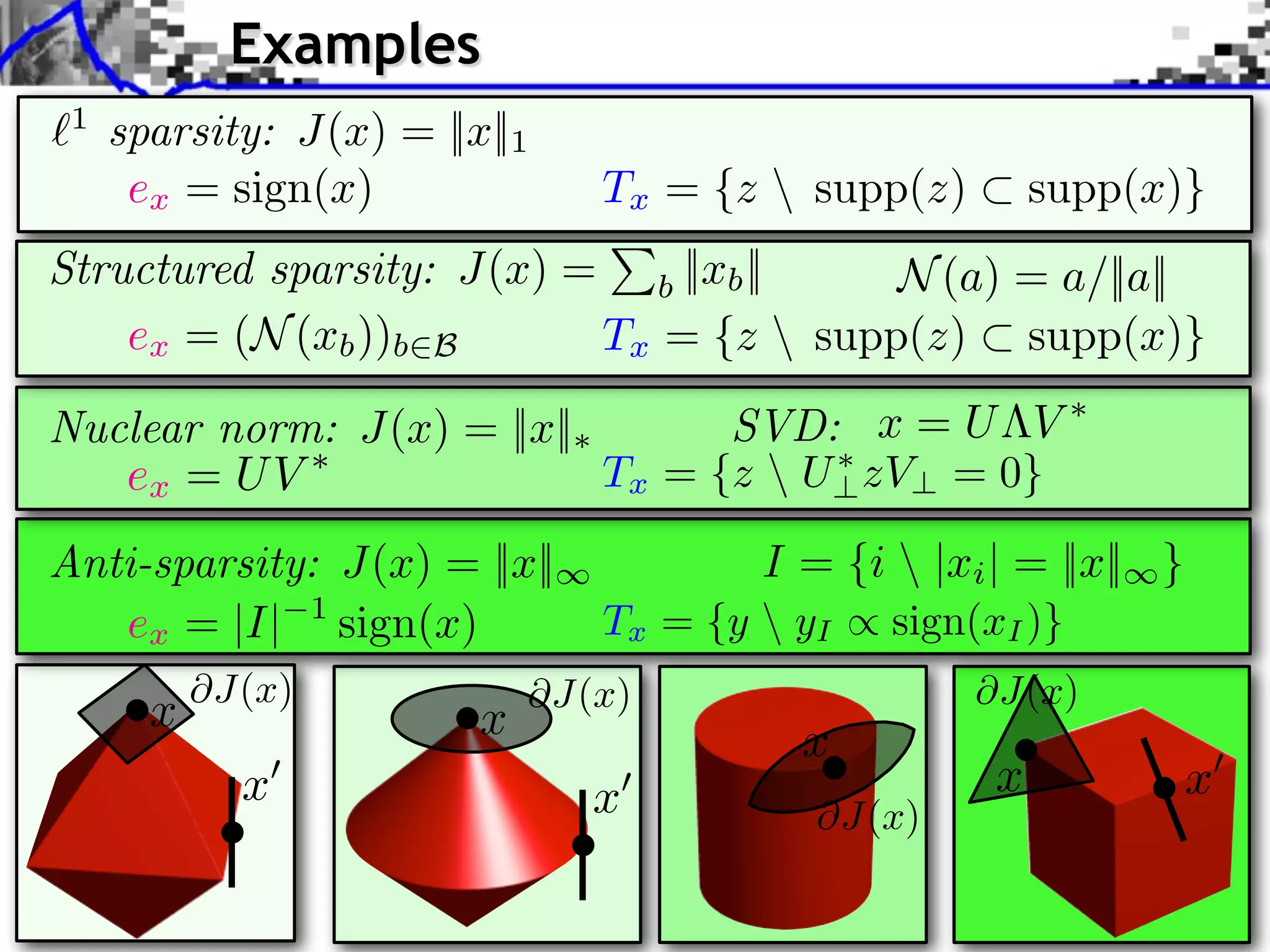
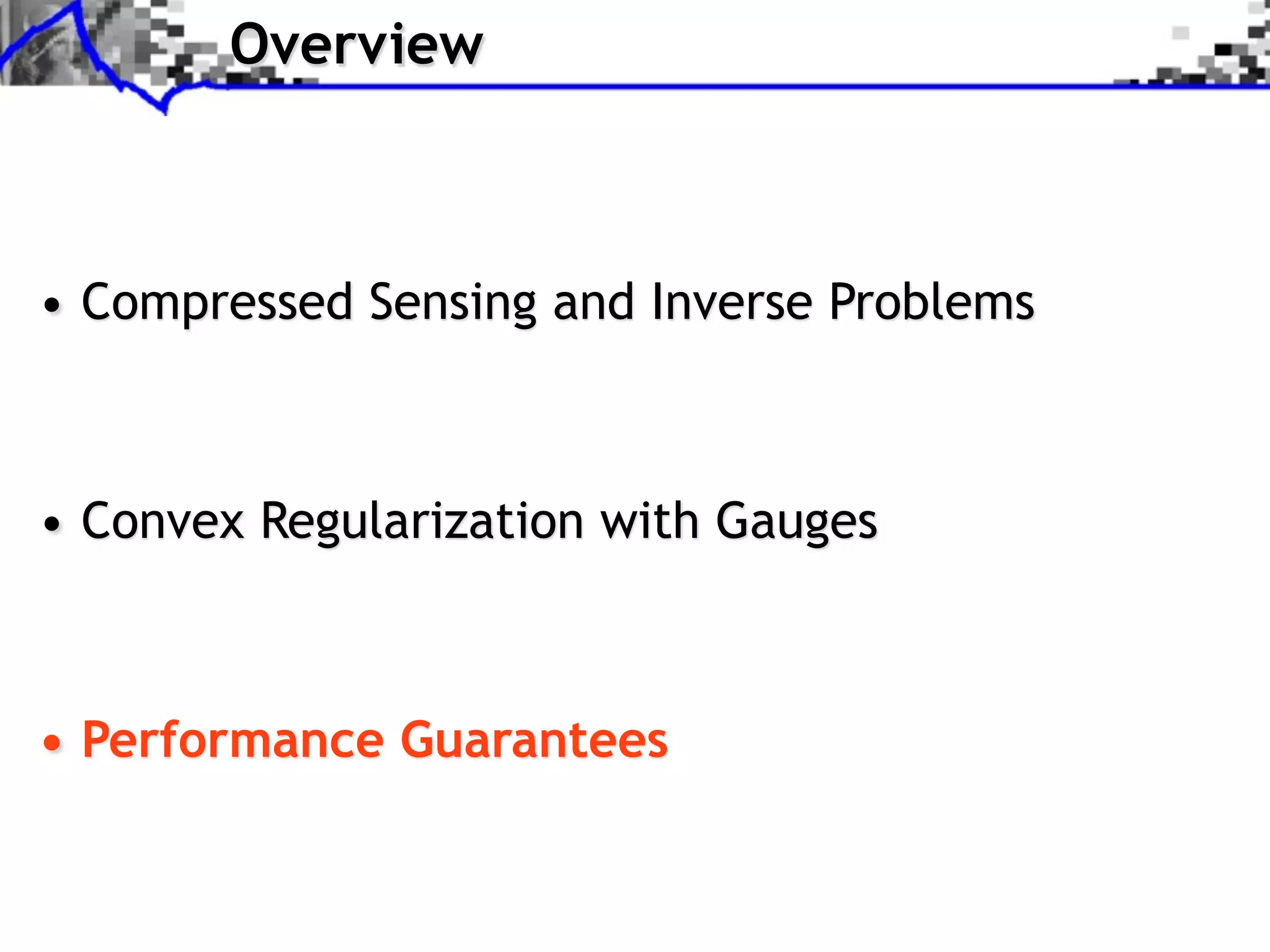
This document discusses regularization techniques for inverse problems. It begins with an overview of compressed sensing and inverse problems, as well as convex regularization using gauges. It then discusses performance guarantees for regularization methods using dual certificates and L2 stability. Specific examples of regularization gauges are given for various models including sparsity, structured sparsity, low-rank, and anti-sparsity. Conditions for exact recovery using random measurements are provided for sparse vectors and low-rank matrices. The discussion concludes with the concept of a minimal-norm certificate for the dual problem.