Signal Processing Course : Convex Optimization

Convex Optimization for Imaging Gabriel Peyré www.numerical-tours.com

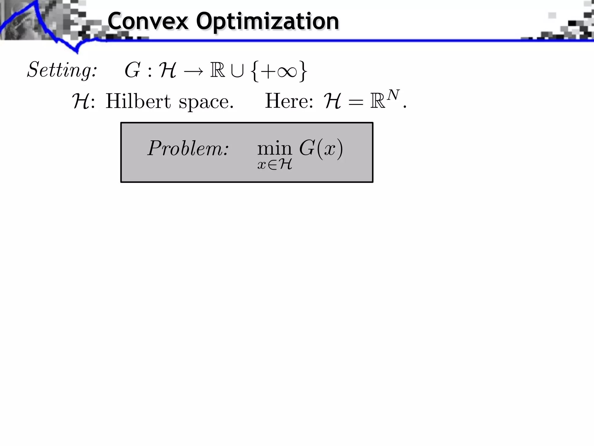
Convex Optimization Setting: G : H R ⇤ {+⇥} H: Hilbert space. Here: H = RN . Problem: min G(x) x H

Convex Optimization Setting: G : H R ⇤ {+⇥} H: Hilbert space. Here: H = RN . Problem: min G(x) x H Class of functions: x y Convex: G(tx + (1 t)y) tG(x) + (1 t)G(y) t [0, 1]

Convex Optimization Setting: G : H R ⇤ {+⇥} H: Hilbert space. Here: H = RN . Problem: min G(x) x H Class of functions: x y Convex: G(tx + (1 t)y) tG(x) + (1 t)G(y) t [0, 1] Lower semi-continuous: lim inf G(x) G(x0 ) x x0 Proper: {x ⇥ H G(x) ⇤= + } = ⌅ ⇤

Convex Optimization Setting: G : H R ⇤ {+⇥} H: Hilbert space. Here: H = RN . Problem: min G(x) x H Class of functions: x y Convex: G(tx + (1 t)y) tG(x) + (1 t)G(y) t [0, 1] Lower semi-continuous: lim inf G(x) G(x0 ) x x0 Proper: {x ⇥ H G(x) ⇤= + } = ⌅ ⇤ 0 if x ⇥ C, Indicator: C (x) = + otherwise. (C closed and convex)

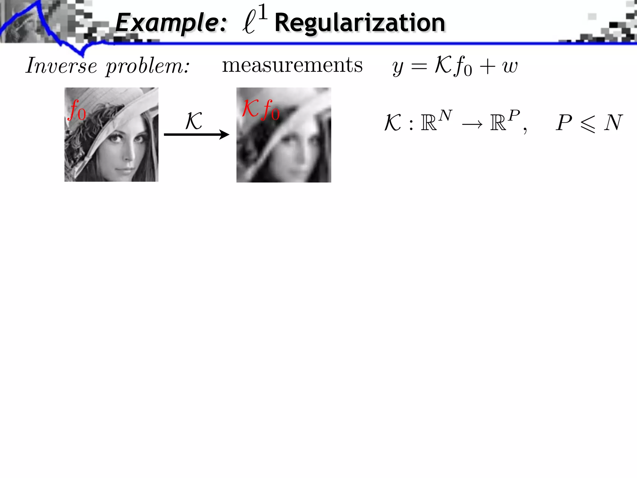
1 Example: Regularization Inverse problem: measurements y = Kf0 + w f0 Kf0 K K : RN RP , P N

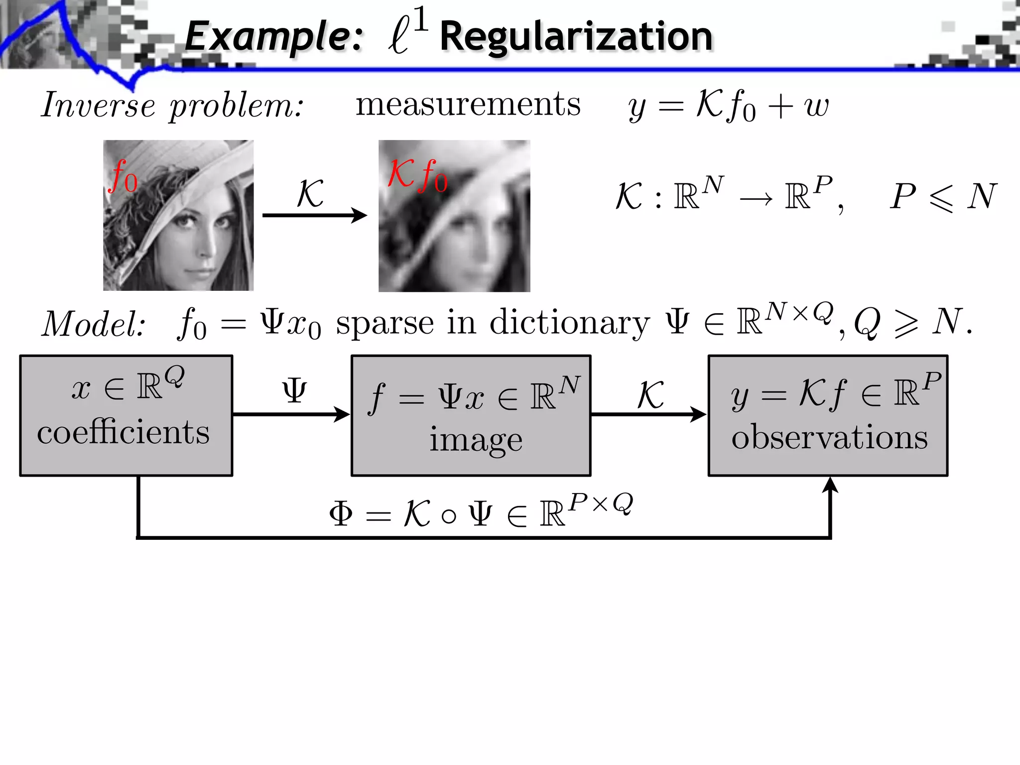
1 Example: Regularization Inverse problem: measurements y = Kf0 + w f0 Kf0 K K : RN RP , P N Model: f0 = x0 sparse in dictionary RN Q ,Q N. x RQ f= x R N K y = Kf RP coe cients image observations = K ⇥ ⇥ RP Q

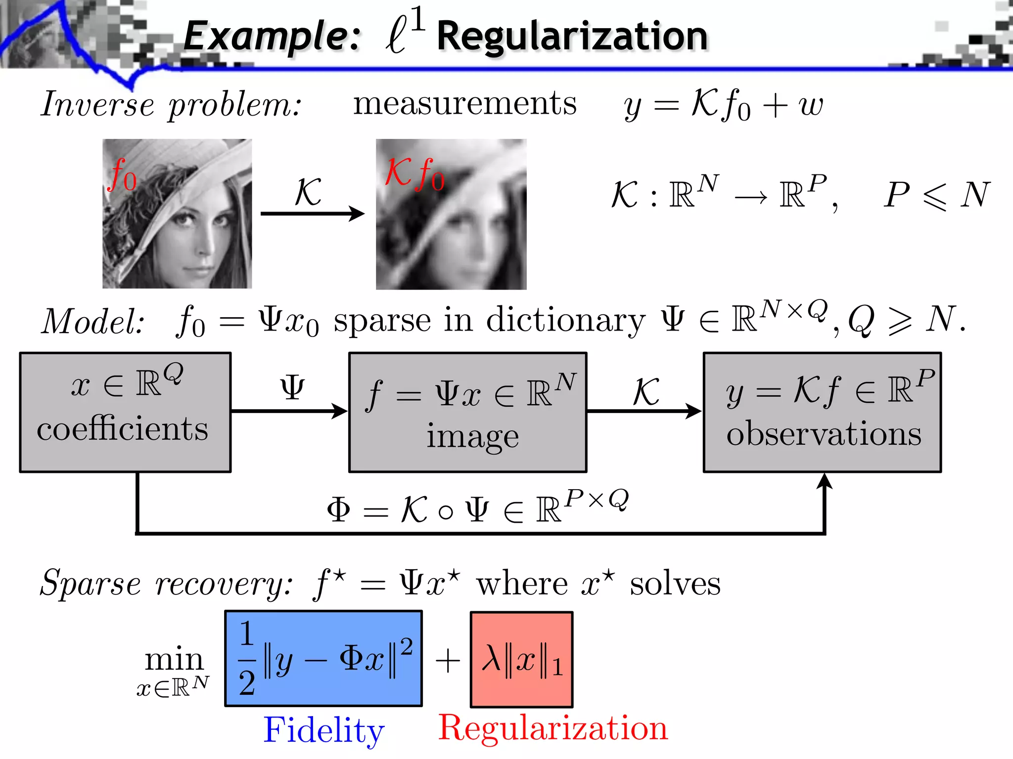
1 Example: Regularization Inverse problem: measurements y = Kf0 + w f0 Kf0 K K : RN RP , P N Model: f0 = x0 sparse in dictionary RN Q ,Q N. x RQ f= x R N K y = Kf RP coe cients image observations = K ⇥ ⇥ RP Q Sparse recovery: f = x where x solves 1 min ||y x||2 + ||x||1 x RN 2 Fidelity Regularization

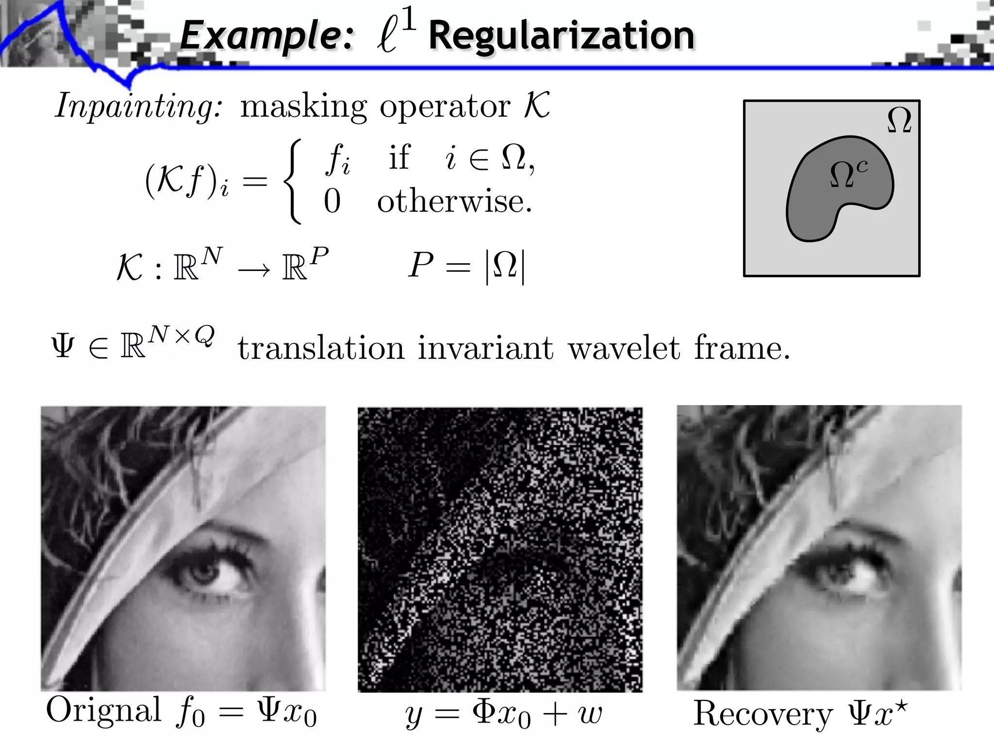
1 Example: Regularization Inpainting: masking operator K fi if i , c (Kf )i = 0 otherwise. K : RN RP P =| | RN Q translation invariant wavelet frame. Orignal f0 = x0 y = x0 + w Recovery x

Overview • Subdifferential Calculus • Proximal Calculus • Forward Backward • Douglas Rachford • Generalized Forward-Backward • Duality

Sub-differential Sub-di erential: G(x) = {u ⇥ H ⇤ z, G(z) G(x) + ⌅u, z x⇧} G(x) = |x| G(0) = [ 1, 1]

Sub-differential Sub-di erential: G(x) = {u ⇥ H ⇤ z, G(z) G(x) + ⌅u, z x⇧} G(x) = |x| Smooth functions: If F is C 1 , F (x) = { F (x)} G(0) = [ 1, 1]

Sub-differential Sub-di erential: G(x) = {u ⇥ H ⇤ z, G(z) G(x) + ⌅u, z x⇧} G(x) = |x| Smooth functions: If F is C 1 , F (x) = { F (x)} G(0) = [ 1, 1] First-order conditions: x argmin G(x) 0 G(x ) x H

Sub-differential Sub-di erential: G(x) = {u ⇥ H ⇤ z, G(z) G(x) + ⌅u, z x⇧} G(x) = |x| Smooth functions: If F is C 1 , F (x) = { F (x)} G(0) = [ 1, 1] First-order conditions: x argmin G(x) 0 G(x ) x H U (x) x Monotone operator: U (x) = G(x) (u, v) U (x) U (y), y x, v u 0

1 Example: Regularization 1 x ⇥ argmin G(x) = ||y x||2 + ||x||1 x RQ 2 ⇥G(x) = ( x y) + ⇥|| · ||1 (x) sign(xi ) if xi ⇥= 0, || · ||1 (x)i = [ 1, 1] if xi = 0.

1 Example: Regularization 1 x ⇥ argmin G(x) = ||y x||2 + ||x||1 x RQ 2 ⇥G(x) = ( x y) + ⇥|| · ||1 (x) sign(xi ) if xi ⇥= 0, xi || · ||1 (x)i = [ 1, 1] if xi = 0. i Support of the solution: I = {i ⇥ {0, . . . , N 1} xi ⇤= 0}

1 Example: Regularization 1 x ⇥ argmin G(x) = ||y x||2 + ||x||1 x RQ 2 ⇥G(x) = ( x y) + ⇥|| · ||1 (x) sign(xi ) if xi ⇥= 0, xi || · ||1 (x)i = [ 1, 1] if xi = 0. i Support of the solution: I = {i ⇥ {0, . . . , N 1} xi ⇤= 0} First-order conditions: i, y x i s RN , ( x y) + s = 0 sI = sign(xI ), ||sI c || 1.

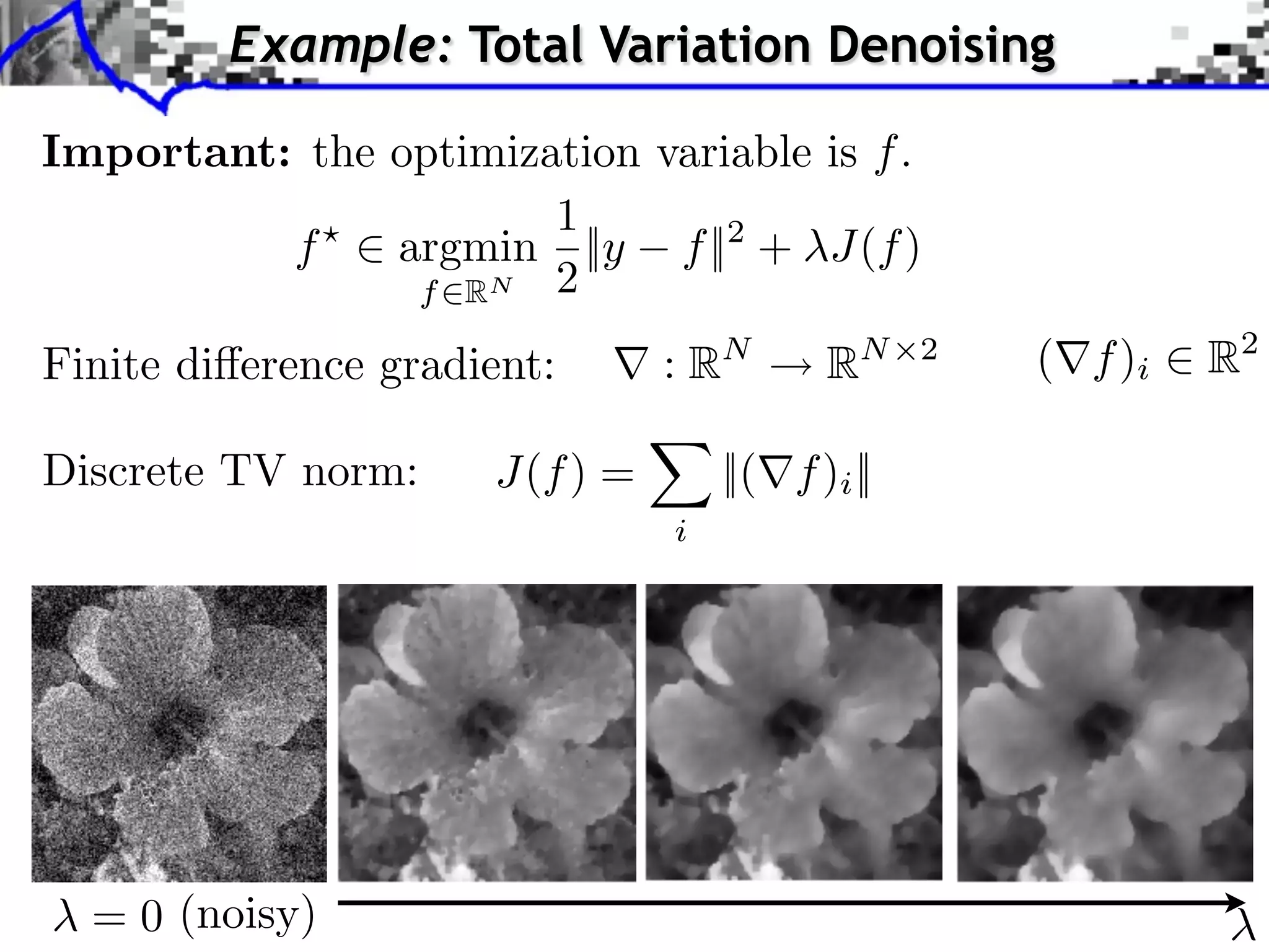
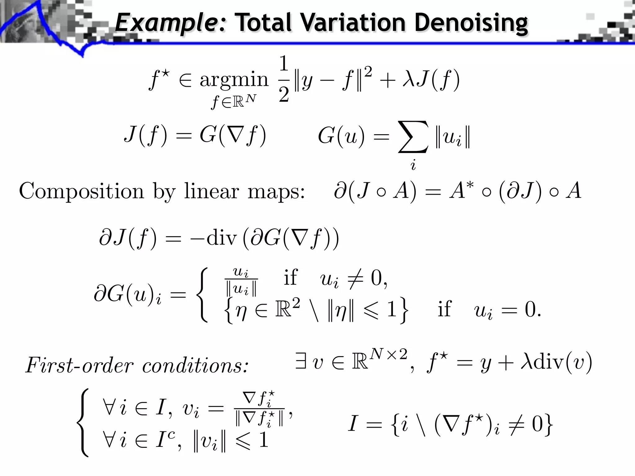
Example: Total Variation Denoising Important: the optimization variable is f . 1 f ⇥ argmin ||y f ||2 + J(f ) f RN 2 Finite di erence gradient: :R N R N 2 ( f )i R2 Discrete TV norm: J(f ) = ||( f )i || i = 0 (noisy)

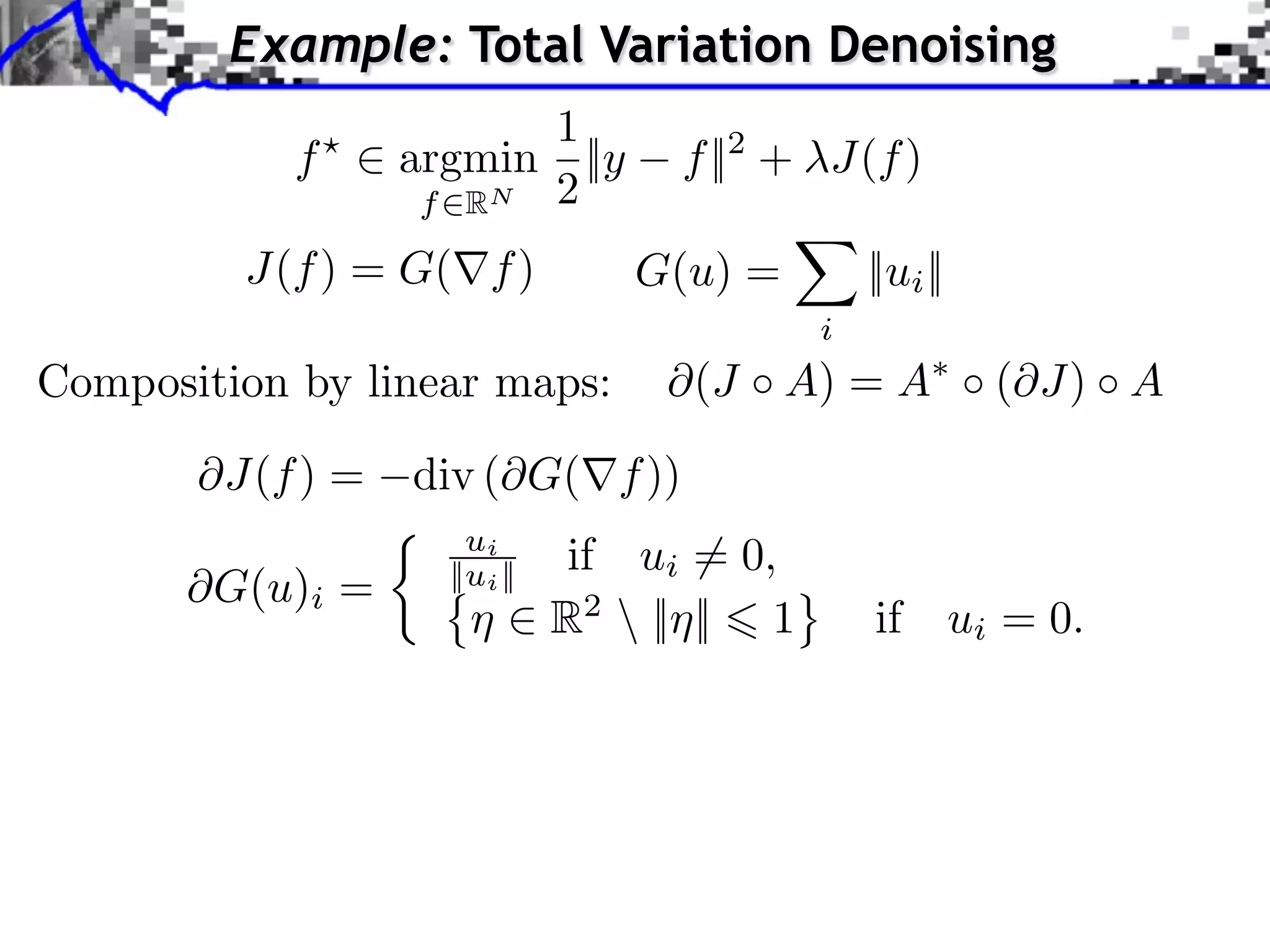
Example: Total Variation Denoising 1 f ⇥ argmin ||y f ||2 + J(f ) f RN 2 J(f ) = G( f ) G(u) = ||ui || i Composition by linear maps: (J A) = A ( J) A J(f ) = div ( G( f )) ui if ui ⇥= 0, ⇥G(u)i = ||ui || R2 || || 1 if ui = 0.

Example: Total Variation Denoising 1 f ⇥ argmin ||y f ||2 + J(f ) f RN 2 J(f ) = G( f ) G(u) = ||ui || i Composition by linear maps: (J A) = A ( J) A J(f ) = div ( G( f )) ui if ui ⇥= 0, ⇥G(u)i = ||ui || R2 || || 1 if ui = 0. First-order conditions: v RN 2 , f = y + div(v) fi ⇥i I, vi = || fi || , I = {i (⇥f )i = 0} ⇥i I c , ||vi || 1

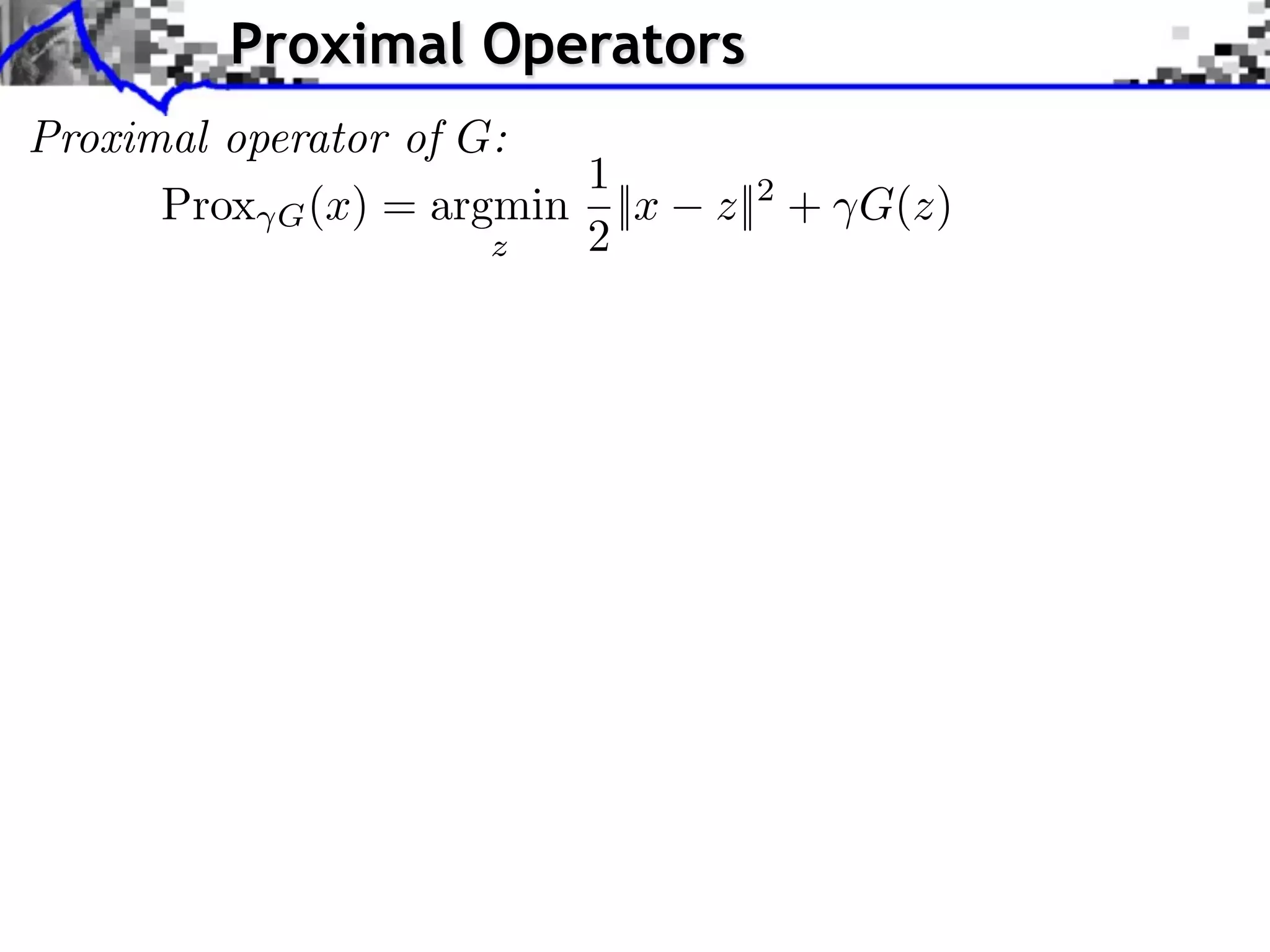
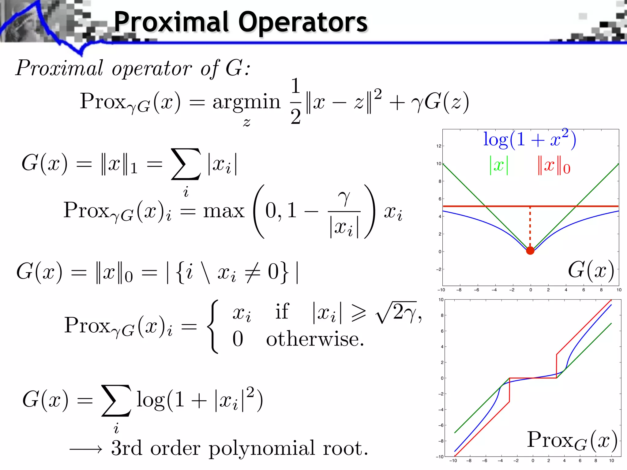
Proximal Operators Proximal operator of G: 1 Prox G (x) = argmin ||x z||2 + G(z) z 2

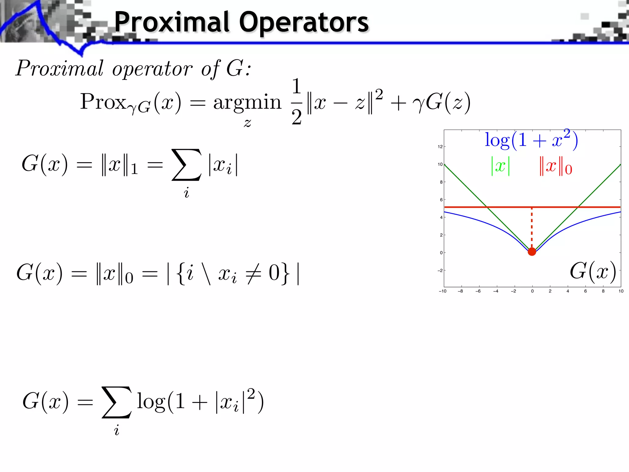
Proximal Operators Proximal operator of G: 1 Prox G (x) = argmin ||x z||2 + G(z) z 2 12 log(1 + x2 ) G(x) = ||x||1 = |xi | 10 |x| ||x||0 8 i 6 4 2 0 G(x) = ||x||0 = | {i xi = 0} | −2 G(x) −10 −8 −6 −4 −2 0 2 4 6 8 10 G(x) = log(1 + |xi |2 ) i

Proximal Operators Proximal operator of G: 1 Prox G (x) = argmin ||x z||2 + G(z) z 2 12 log(1 + x2 ) G(x) = ||x||1 = |xi | 10 |x| ||x||0 8 i Prox G (x)i = max 0, 1 6 xi 4 |xi | 2 0 G(x) = ||x||0 = | {i xi = 0} | −2 G(x) −10 −8 −6 −4 −2 0 2 4 6 8 10 xi if |xi | 2 , 10 Prox G (x)i = 8 0 otherwise. 6 4 2 0 G(x) = log(1 + |xi |2 ) −2 −4 i −6 3rd order polynomial root. −8 ProxG (x) −10 −10 −8 −6 −4 −2 0 2 4 6 8 10

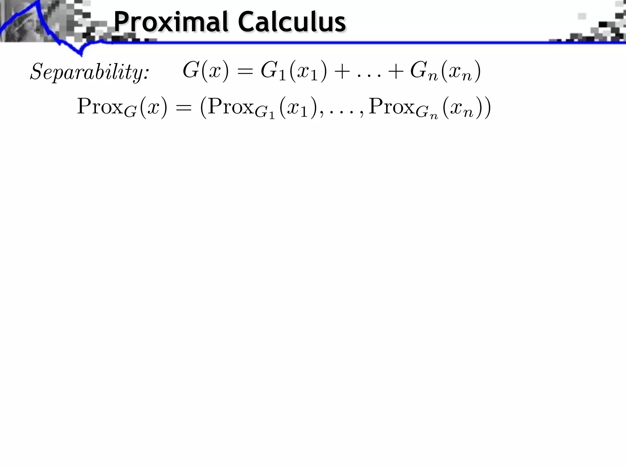
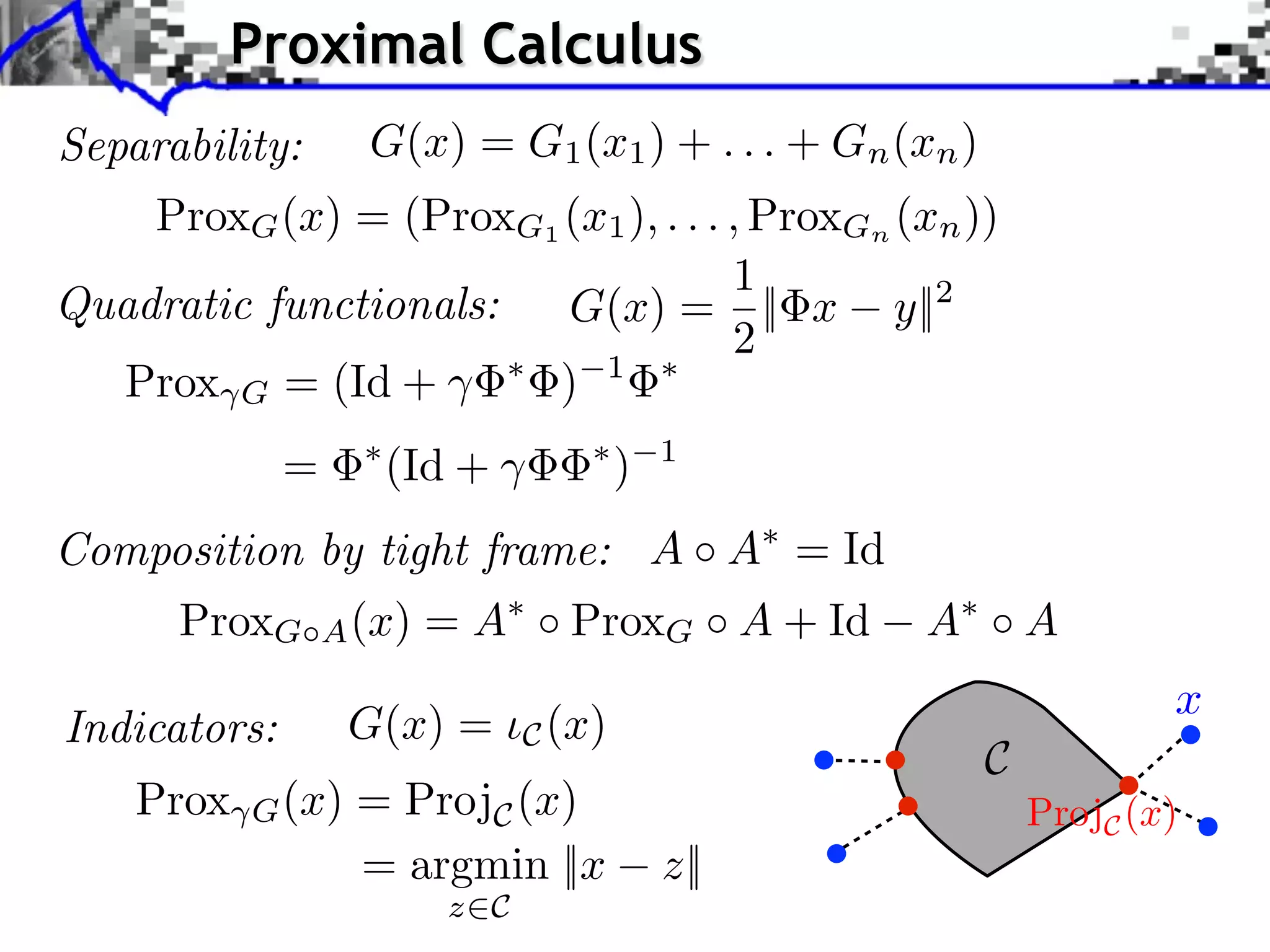
Proximal Calculus Separability: G(x) = G1 (x1 ) + . . . + Gn (xn ) ProxG (x) = (ProxG1 (x1 ), . . . , ProxGn (xn ))

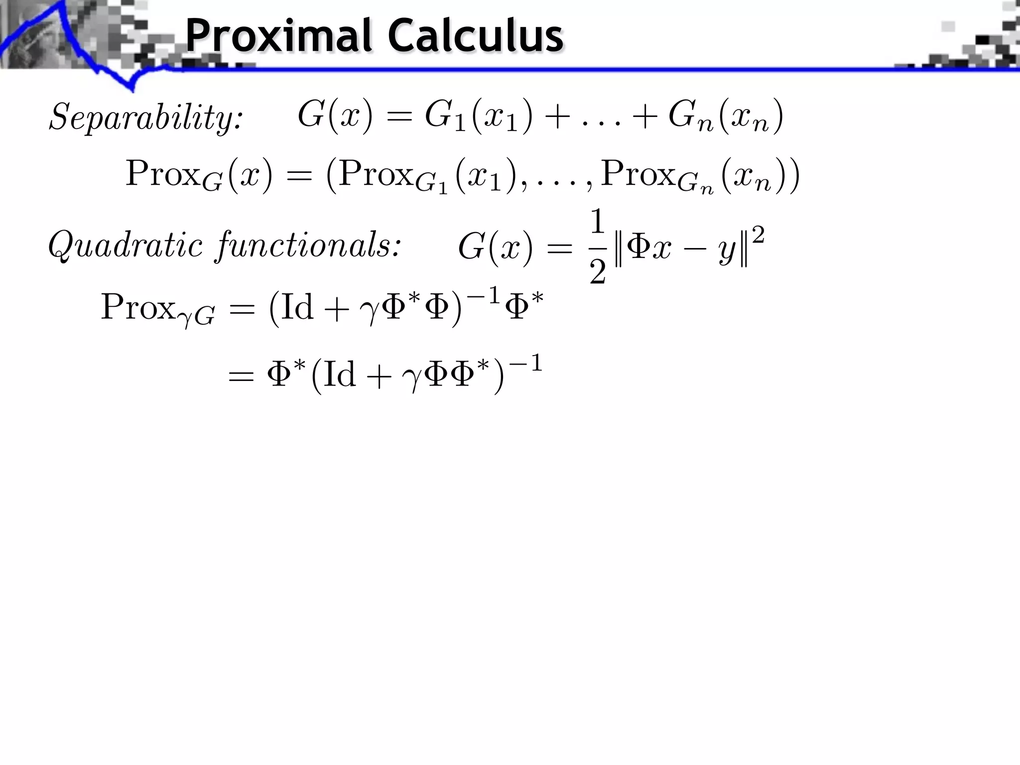
Proximal Calculus Separability: G(x) = G1 (x1 ) + . . . + Gn (xn ) ProxG (x) = (ProxG1 (x1 ), . . . , ProxGn (xn )) 1 Quadratic functionals: G(x) = || x y||2 2 Prox G = (Id + ) 1 = (Id + ) 1

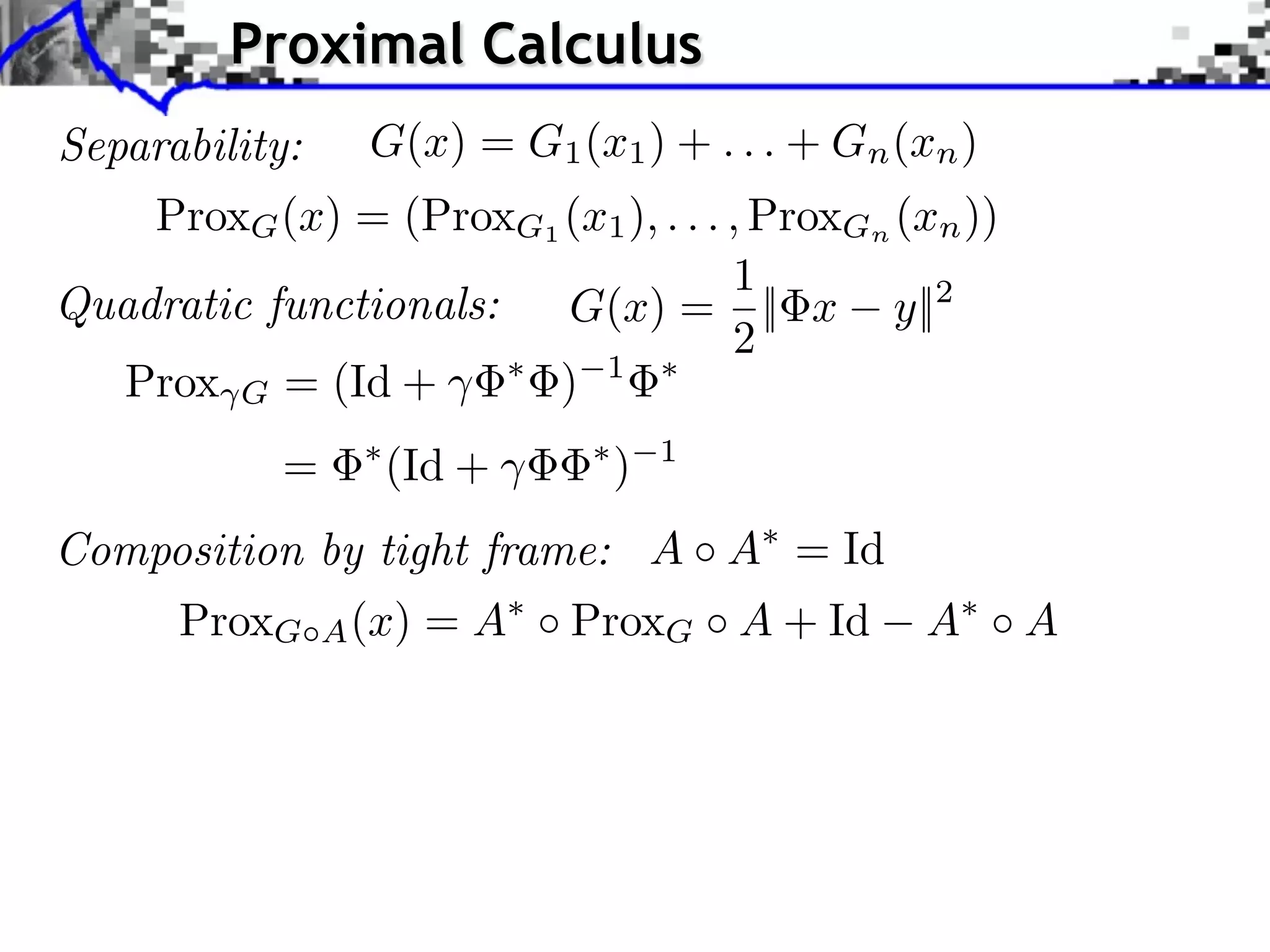
Proximal Calculus Separability: G(x) = G1 (x1 ) + . . . + Gn (xn ) ProxG (x) = (ProxG1 (x1 ), . . . , ProxGn (xn )) 1 Quadratic functionals: G(x) = || x y||2 2 Prox G = (Id + ) 1 = (Id + ) 1 Composition by tight frame: A A = Id ProxG A (x) =A ProxG A + Id A A

Proximal Calculus Separability: G(x) = G1 (x1 ) + . . . + Gn (xn ) ProxG (x) = (ProxG1 (x1 ), . . . , ProxGn (xn )) 1 Quadratic functionals: G(x) = || x y||2 2 Prox G = (Id + ) 1 = (Id + ) 1 Composition by tight frame: A A = Id ProxG A (x) =A ProxG A + Id A A x Indicators: G(x) = C (x) C Prox G (x) = ProjC (x) ProjC (x) = argmin ||x z|| z C

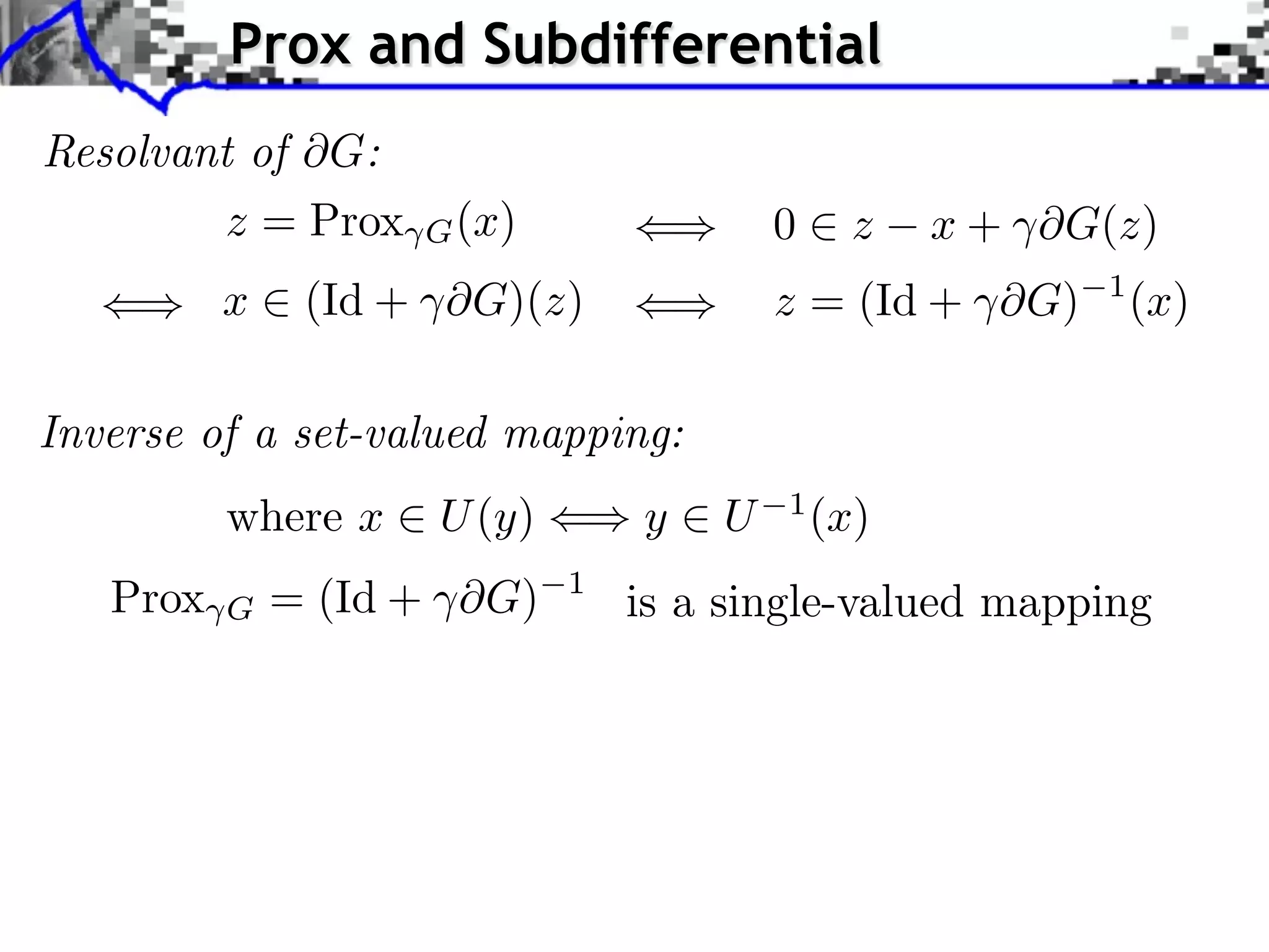
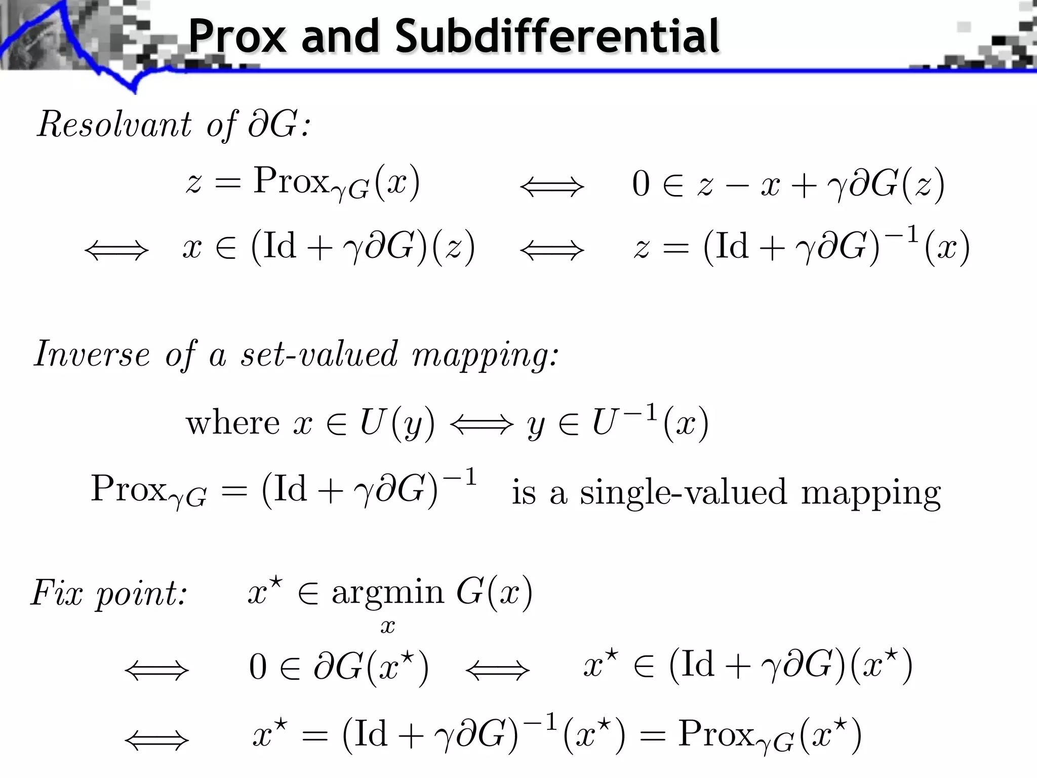
Prox and Subdifferential Resolvant of G: z = Prox G (x) 0 z x + ⇥G(z) x (Id + ⇥G)(z) z = (Id + ⇥G) 1 (x) Inverse of a set-valued mapping: where x U (y) y U 1 (x) Prox G = (Id + ⇥G) 1 is a single-valued mapping

Prox and Subdifferential Resolvant of G: z = Prox G (x) 0 z x + ⇥G(z) x (Id + ⇥G)(z) z = (Id + ⇥G) 1 (x) Inverse of a set-valued mapping: where x U (y) y U 1 (x) Prox G = (Id + ⇥G) 1 is a single-valued mapping Fix point: x argmin G(x) x 0 G(x ) x (Id + ⇥G)(x ) x⇥ = (Id + ⇥G) 1 (x⇥ ) = Prox G (x⇥ )

Gradient and Proximal Descents Gradient descent: x( +1) = x( ) G(x( ) ) [explicit] G is C 1 and G is L-Lipschitz Theorem: If 0 < < 2/L, x( ) x a solution.

Gradient and Proximal Descents Gradient descent: x( +1) = x( ) G(x( ) ) [explicit] G is C 1 and G is L-Lipschitz Theorem: If 0 < < 2/L, x( ) x a solution. Sub-gradient descent: x( +1) = x( ) v( ) , v( ) G(x( ) ) Theorem: If 1/⇥, x( ) x a solution. Problem: slow.

Gradient and Proximal Descents Gradient descent: x( +1) = x( ) G(x( ) ) [explicit] G is C 1 and G is L-Lipschitz Theorem: If 0 < < 2/L, x( ) x a solution. Sub-gradient descent: x( +1) = x( ) v( ) , v( ) G(x( ) ) Theorem: If 1/⇥, x( ) x a solution. Problem: slow. Proximal-point algorithm: x(⇥+1) = Prox G (x(⇥) ) [implicit] Theorem: If c > 0, x( ) x a solution. Prox G hard to compute.

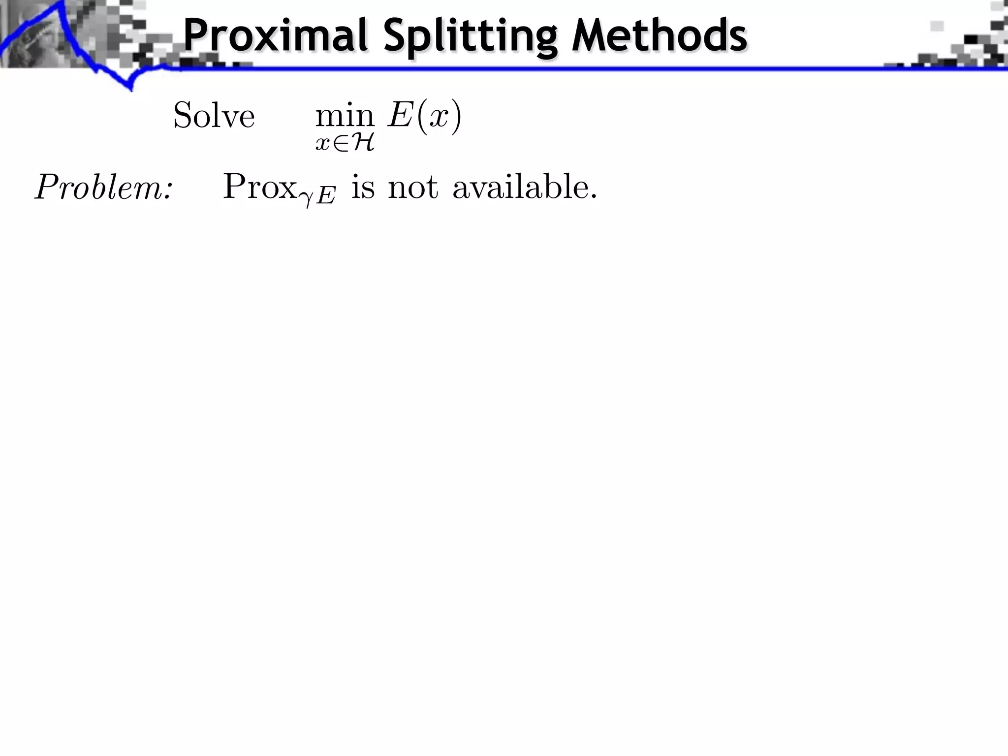
Proximal Splitting Methods Solve min E(x) x H Problem: Prox E is not available.

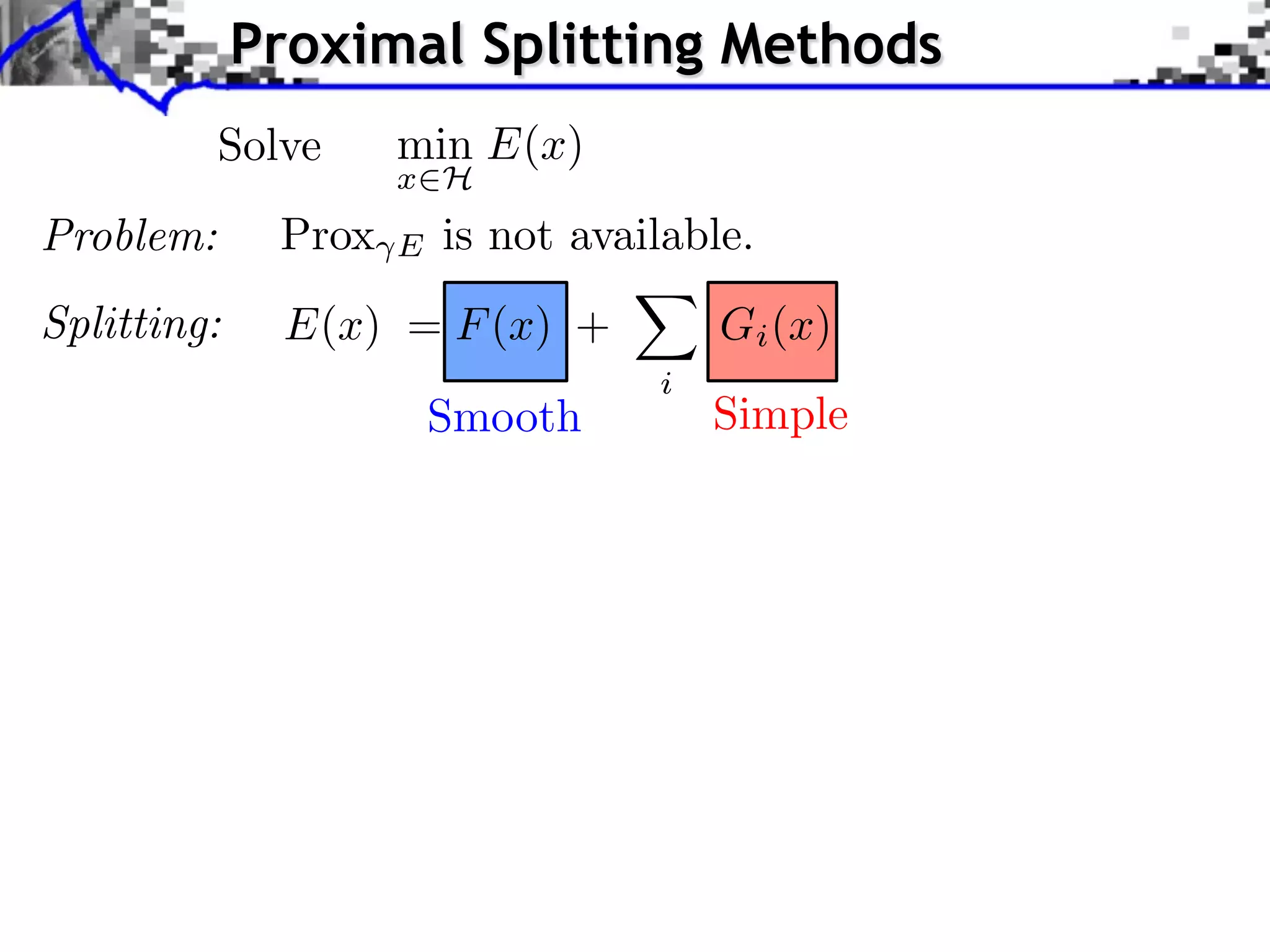
Proximal Splitting Methods Solve min E(x) x H Problem: Prox E is not available. Splitting: E(x) = F (x) + Gi (x) i Smooth Simple

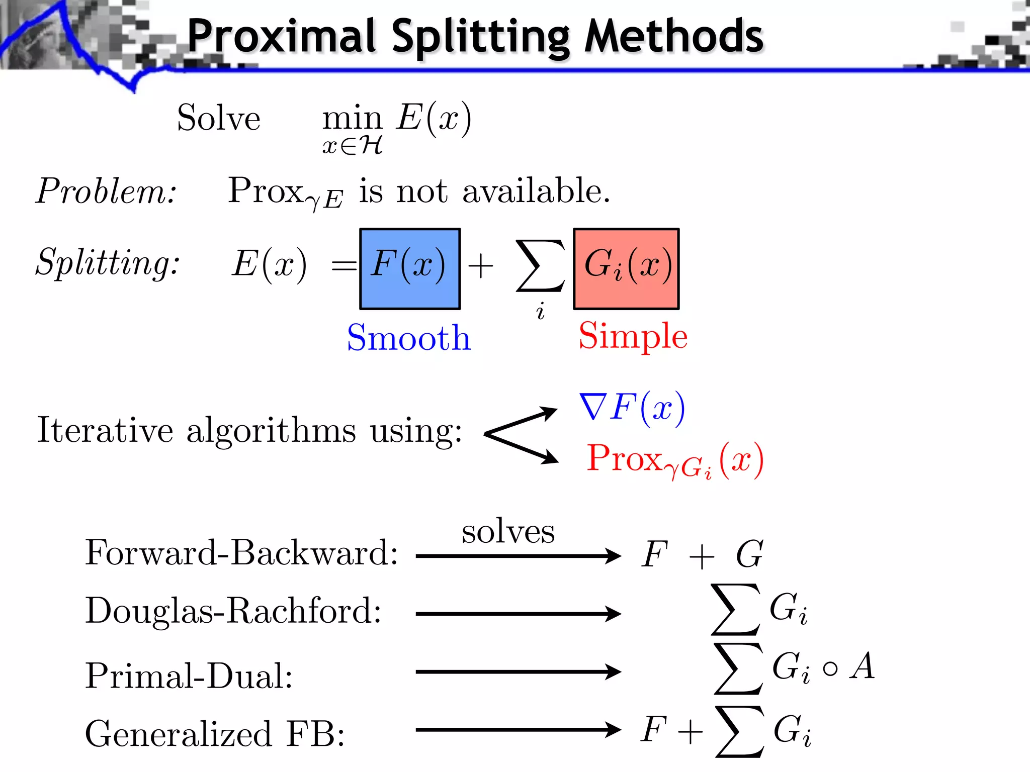
Proximal Splitting Methods Solve min E(x) x H Problem: Prox E is not available. Splitting: E(x) = F (x) + Gi (x) i Smooth Simple F (x) Iterative algorithms using: Prox Gi (x) solves Forward-Backward: F + G Douglas-Rachford: Gi Primal-Dual: Gi A Generalized FB: F+ Gi

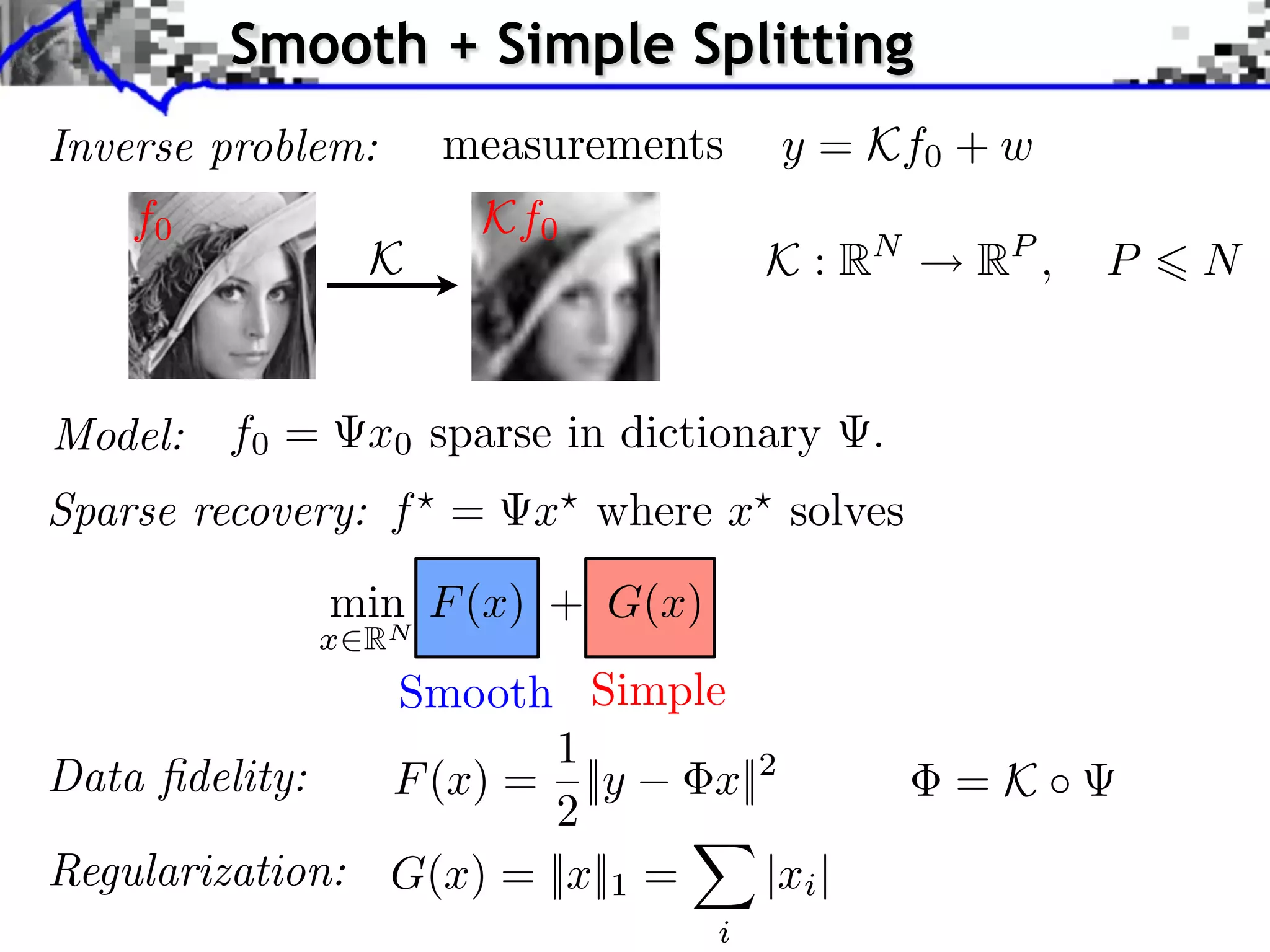
Smooth + Simple Splitting Inverse problem: measurements y = Kf0 + w f0 Kf0 K K : RN RP , P N Model: f0 = x0 sparse in dictionary . Sparse recovery: f = x where x solves min F (x) + G(x) x RN Smooth Simple 1 Data ﬁdelity: F (x) = ||y x||2 =K ⇥ 2 Regularization: G(x) = ||x||1 = |xi | i

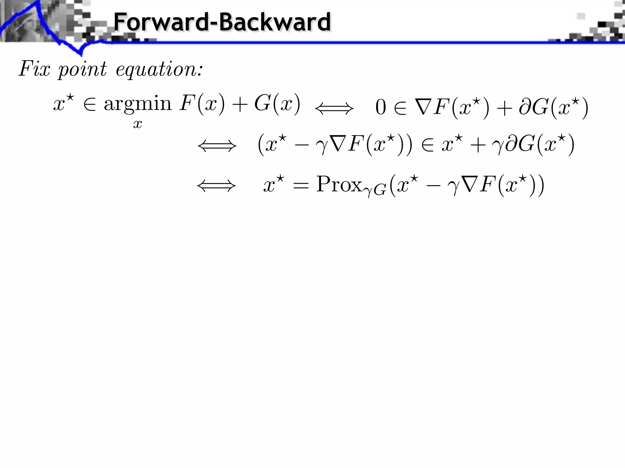
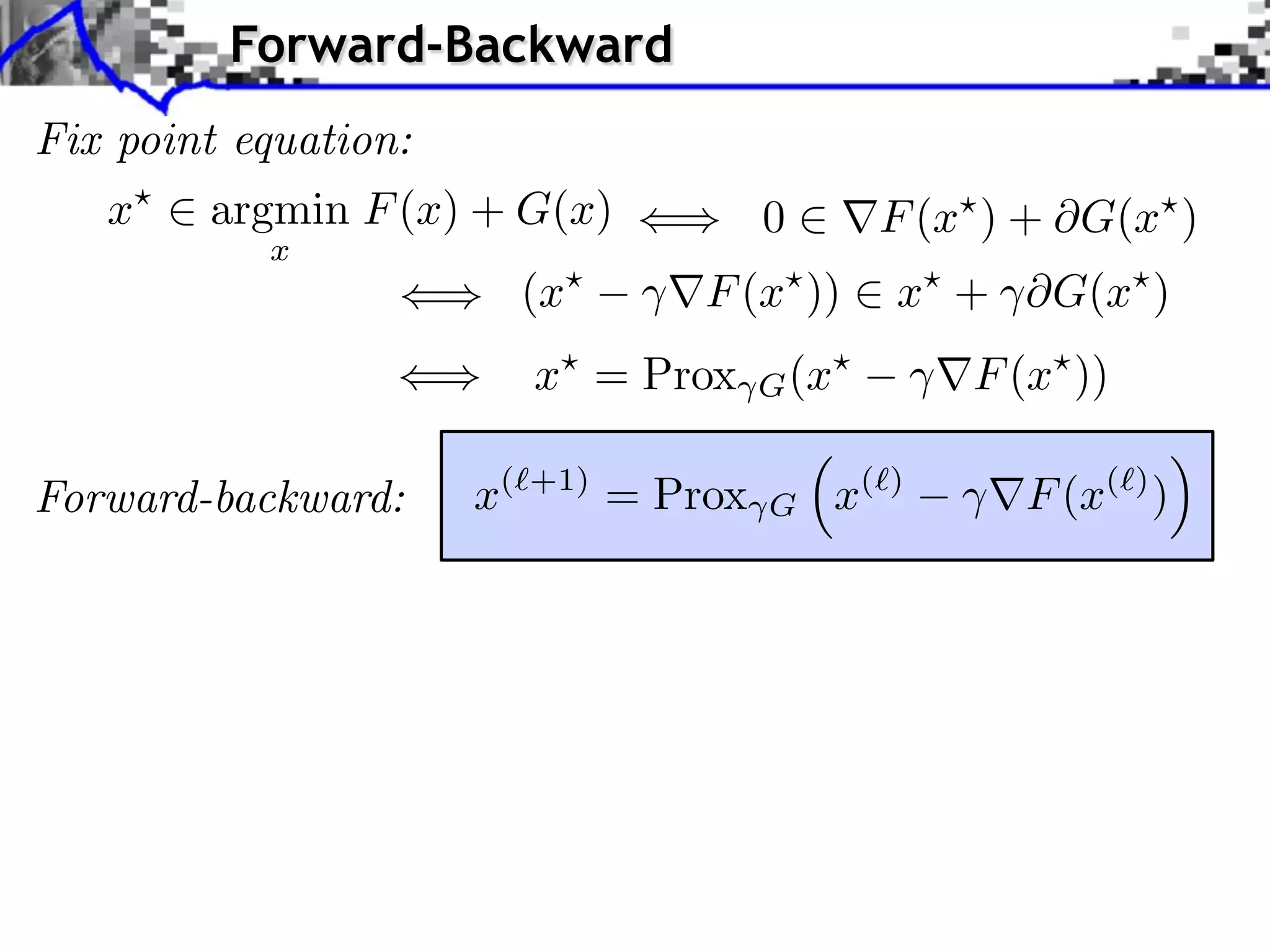
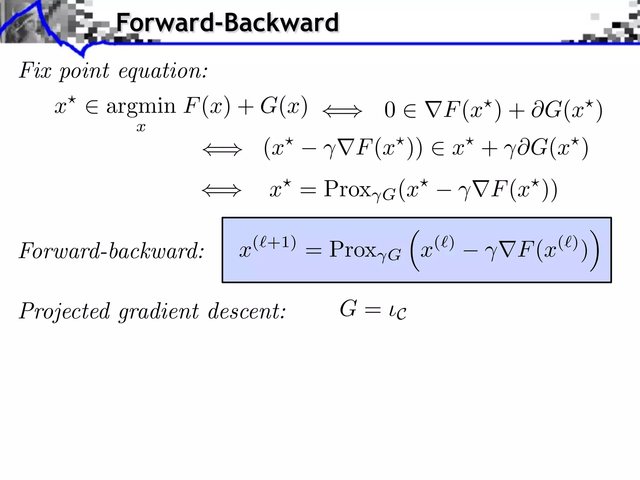
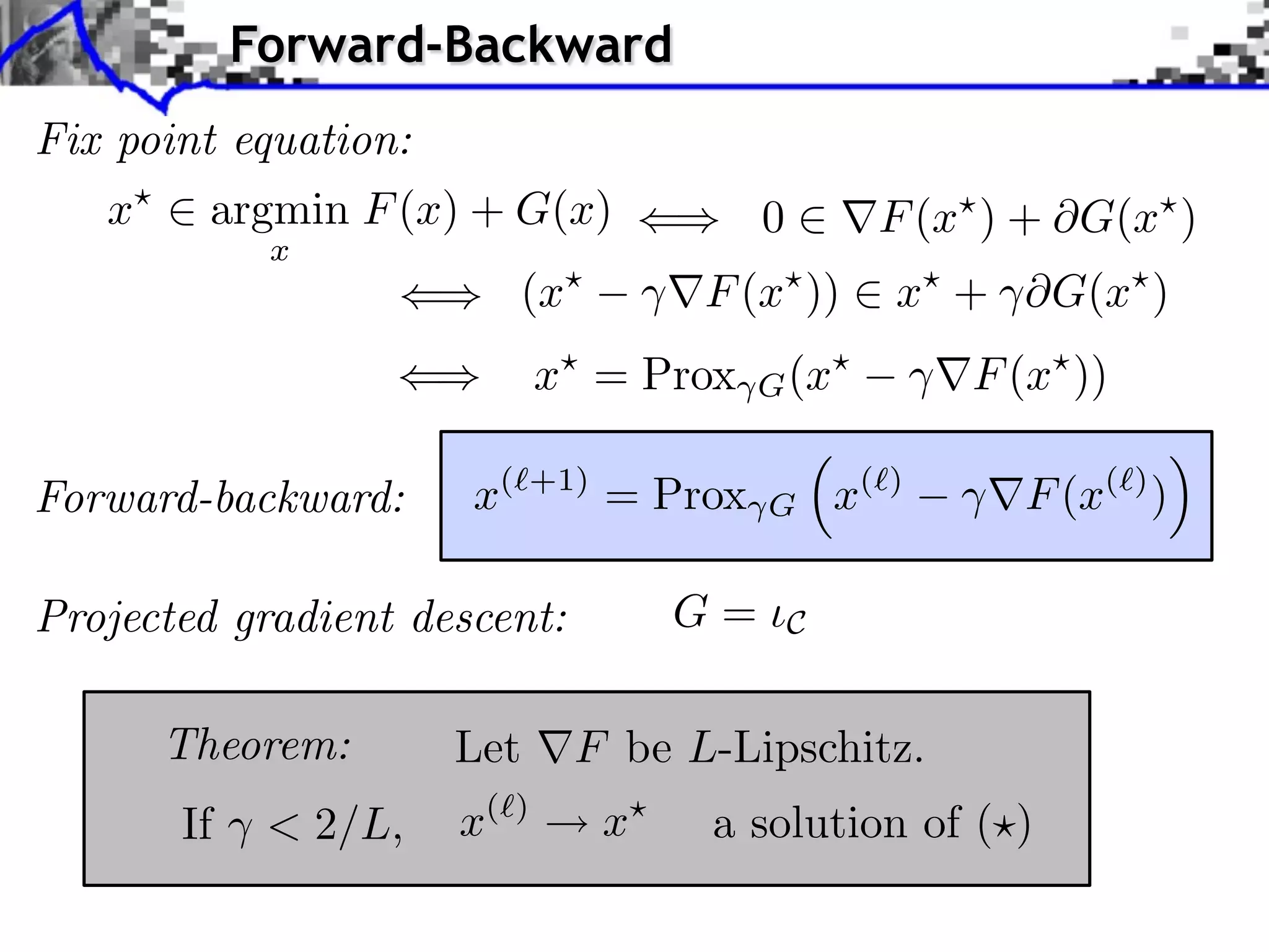
Forward-Backward Fix point equation: x argmin F (x) + G(x) 0 F (x ) + G(x ) x (x F (x )) x + ⇥G(x ) x⇥ = Prox G (x⇥ F (x⇥ ))

Forward-Backward Fix point equation: x argmin F (x) + G(x) 0 F (x ) + G(x ) x (x F (x )) x + ⇥G(x ) x⇥ = Prox G (x⇥ F (x⇥ )) Forward-backward: x(⇥+1) = Prox G x(⇥) F (x(⇥) )

Forward-Backward Fix point equation: x argmin F (x) + G(x) 0 F (x ) + G(x ) x (x F (x )) x + ⇥G(x ) x⇥ = Prox G (x⇥ F (x⇥ )) Forward-backward: x(⇥+1) = Prox G x(⇥) F (x(⇥) ) Projected gradient descent: G= C

Forward-Backward Fix point equation: x argmin F (x) + G(x) 0 F (x ) + G(x ) x (x F (x )) x + ⇥G(x ) x⇥ = Prox G (x⇥ F (x⇥ )) Forward-backward: x(⇥+1) = Prox G x(⇥) F (x(⇥) ) Projected gradient descent: G= C Theorem: Let F be L-Lipschitz. If < 2/L, x( ) x a solution of ( )

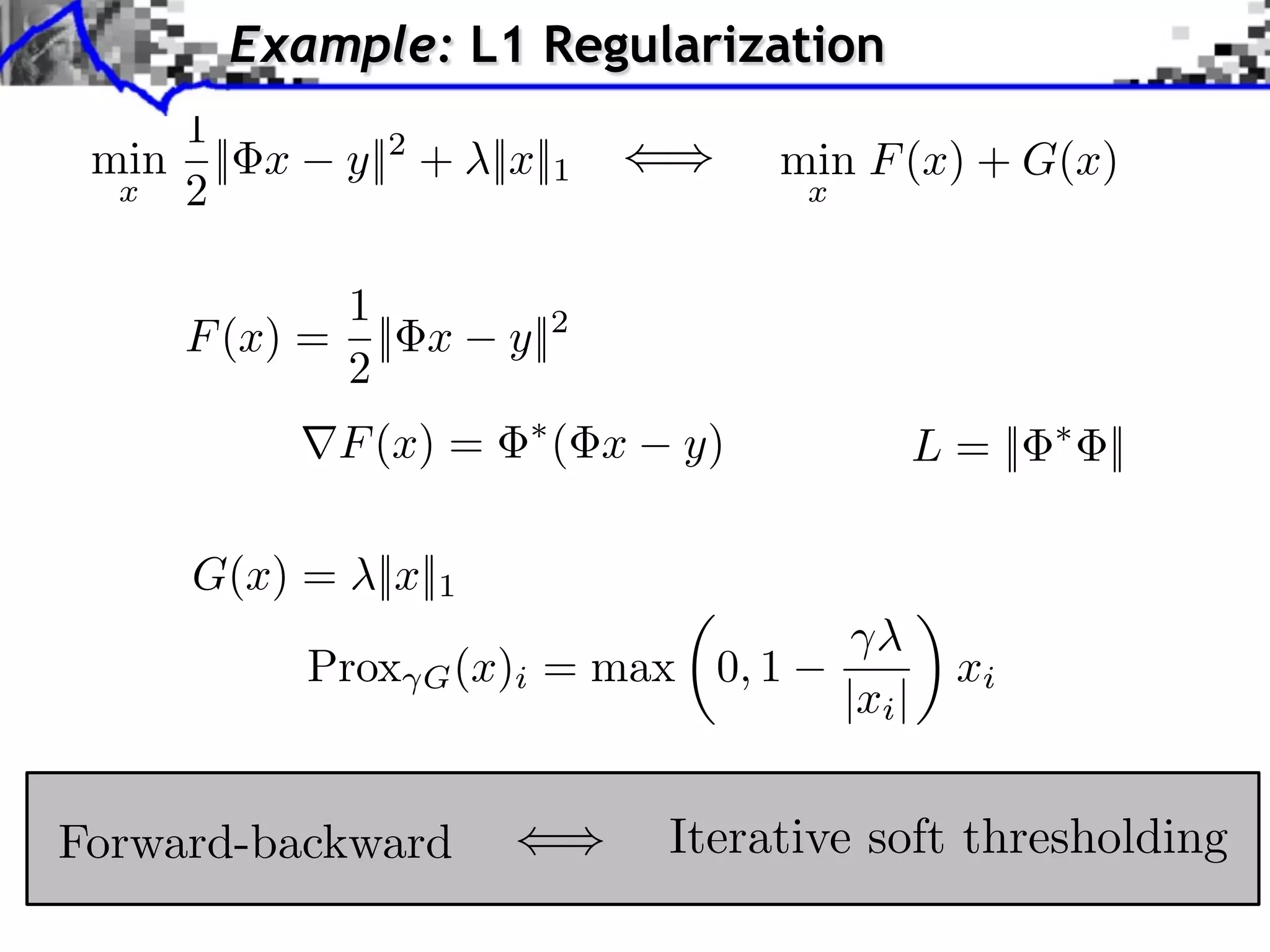
Example: L1 Regularization 1 min || x y||2 + ||x||1 min F (x) + G(x) x 2 x 1 F (x) = || x y||2 2 F (x) = ( x y) L = || || G(x) = ||x||1 ⇥ Prox G (x)i = max 0, 1 xi |xi | Forward-backward Iterative soft thresholding

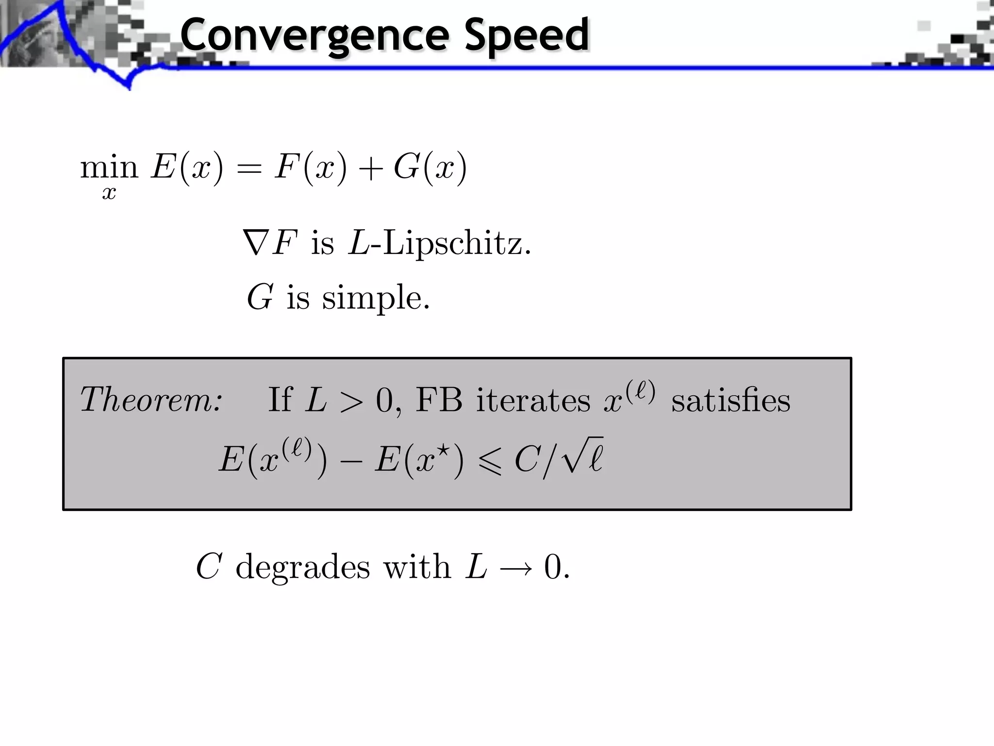
Convergence Speed min E(x) = F (x) + G(x) x F is L-Lipschitz. G is simple. Theorem: If L > 0, FB iterates x( ) satisﬁes E(x( ) ) E(x ) C/ C degrades with L 0.

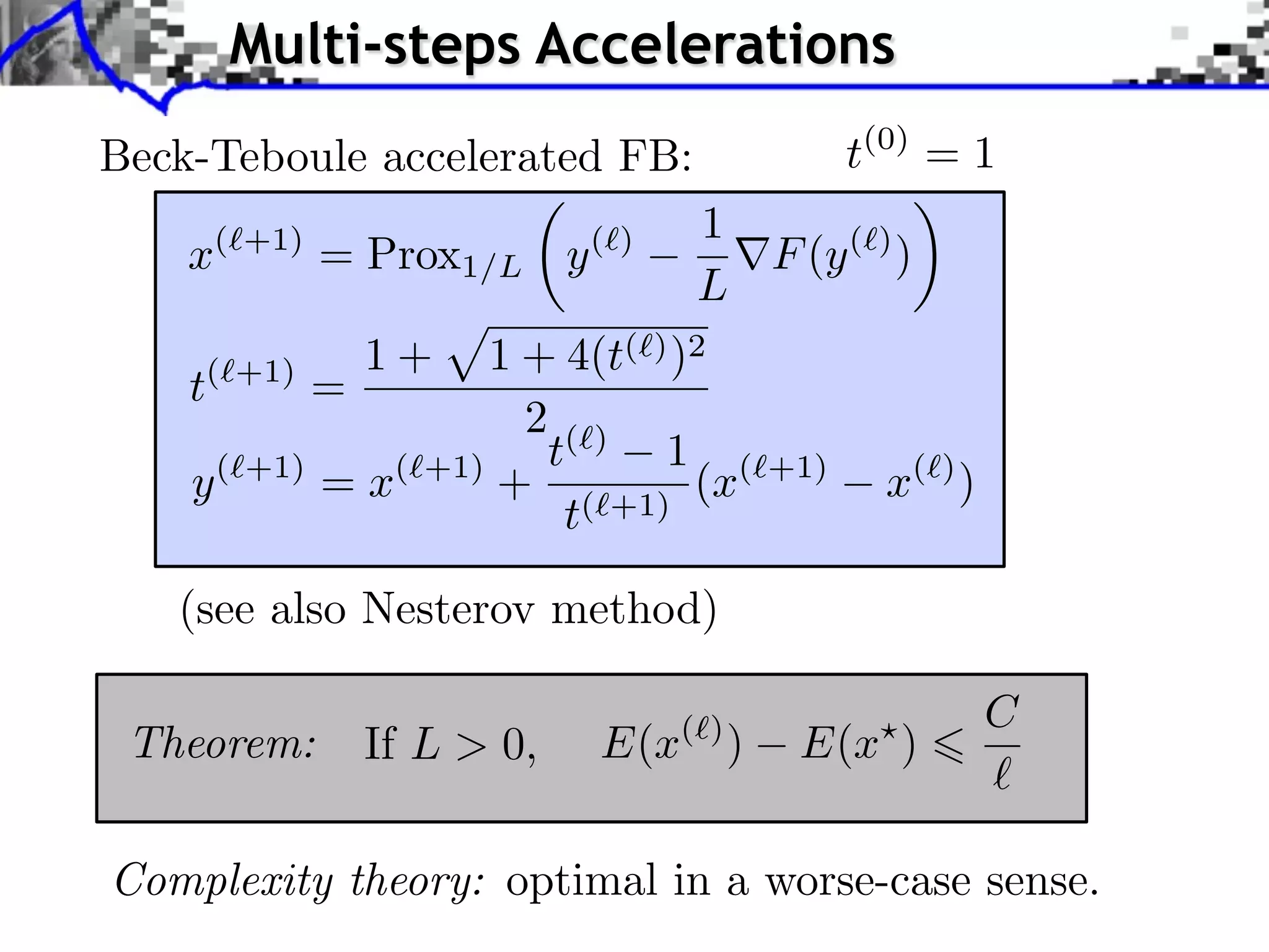
Multi-steps Accelerations Beck-Teboule accelerated FB: t(0) = 1 ✓ ◆ (`+1) (`) 1 x = Prox1/L y rF (y (`) ) L 1+ 1 + 4(t( ) )2 t( +1) = 2() t 1 ( y ( +1) =x( +1) + ( +1) (x +1) x( ) ) t (see also Nesterov method) C Theorem: If L > 0, E(x ( ) ) E(x ) Complexity theory: optimal in a worse-case sense.

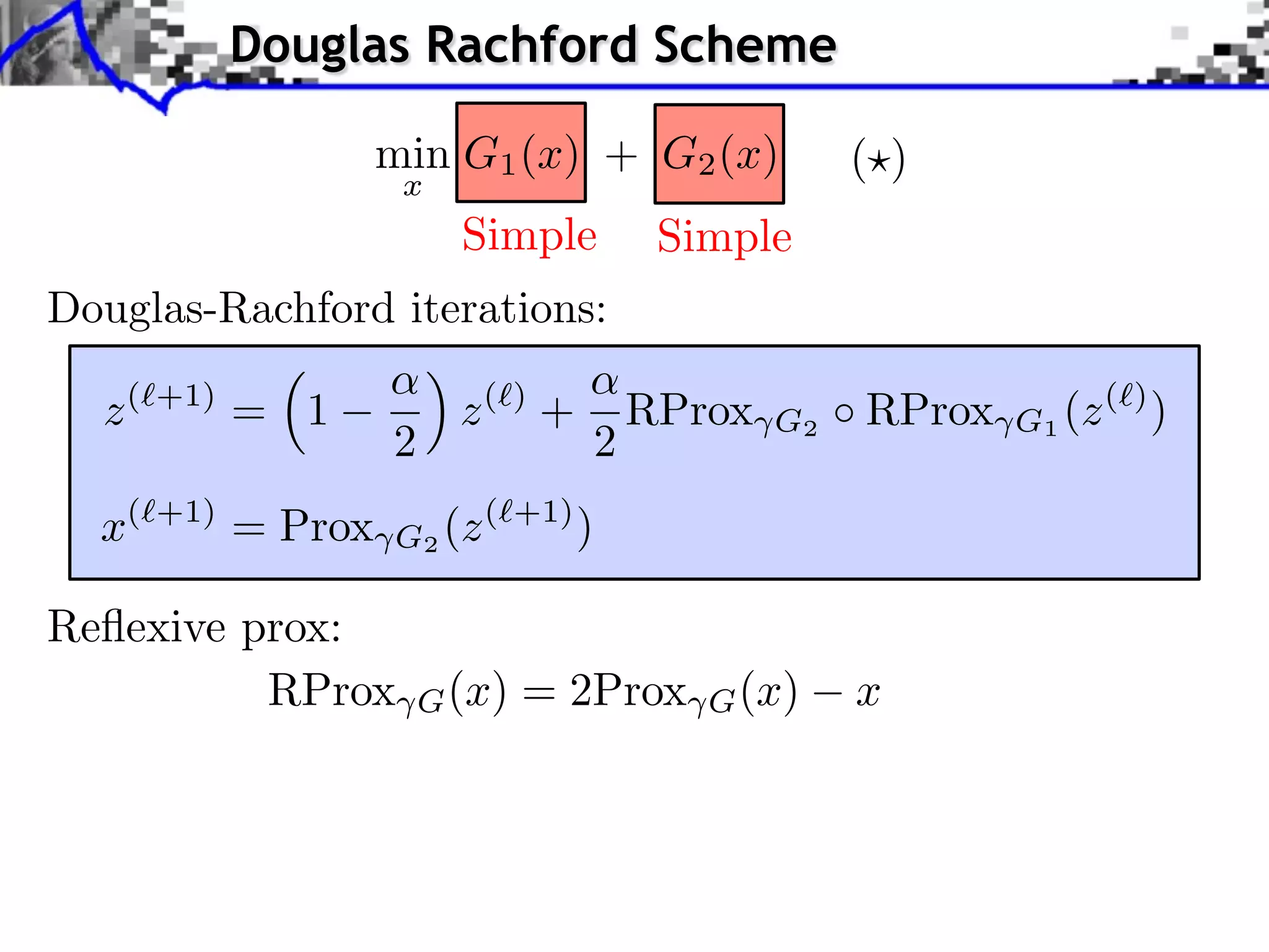
Douglas Rachford Scheme min G1 (x) + G2 (x) ( ) x Simple Simple Douglas-Rachford iterations: z (⇥+1) = 1 z (⇥) + RProx G2 RProx G1 (z (⇥) ) 2 2 x(⇥+1) = Prox G2 (z (⇥+1) ) Reﬂexive prox: RProx G (x) = 2Prox G (x) x

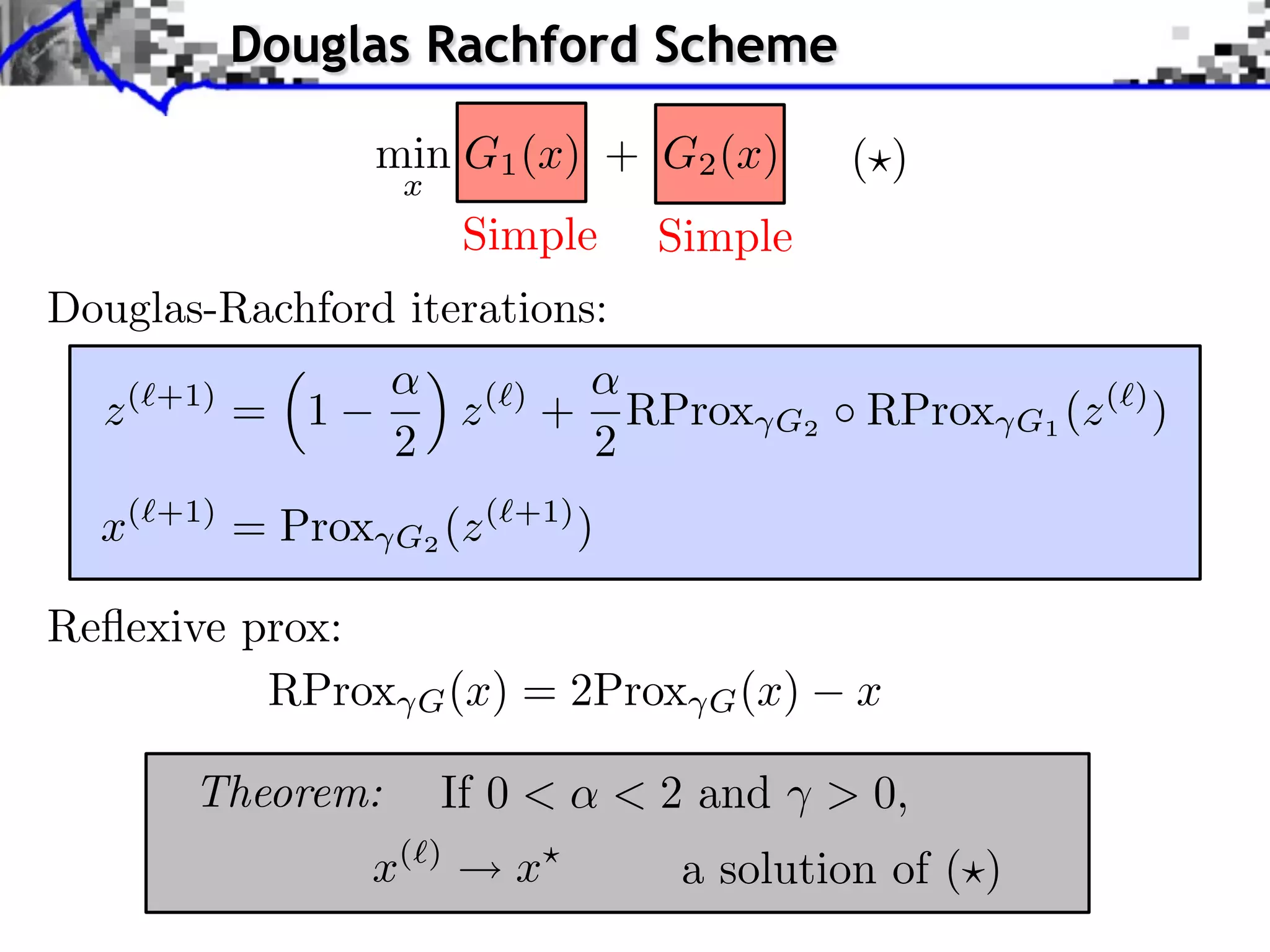
Douglas Rachford Scheme min G1 (x) + G2 (x) ( ) x Simple Simple Douglas-Rachford iterations: z (⇥+1) = 1 z (⇥) + RProx G2 RProx G1 (z (⇥) ) 2 2 x(⇥+1) = Prox G2 (z (⇥+1) ) Reﬂexive prox: RProx G (x) = 2Prox G (x) x Theorem: If 0 < < 2 and ⇥ > 0, x( ) x a solution of ( )

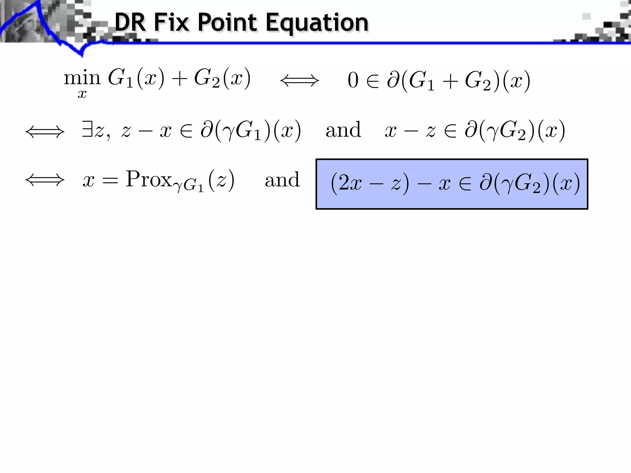
DR Fix Point Equation min G1 (x) + G2 (x) 0 (G1 + G2 )(x) x z, z x ⇥( G1 )(x) and x z ⇥( G2 )(x) x = Prox G1 (z) and (2x z) x ⇥( G2 )(x)

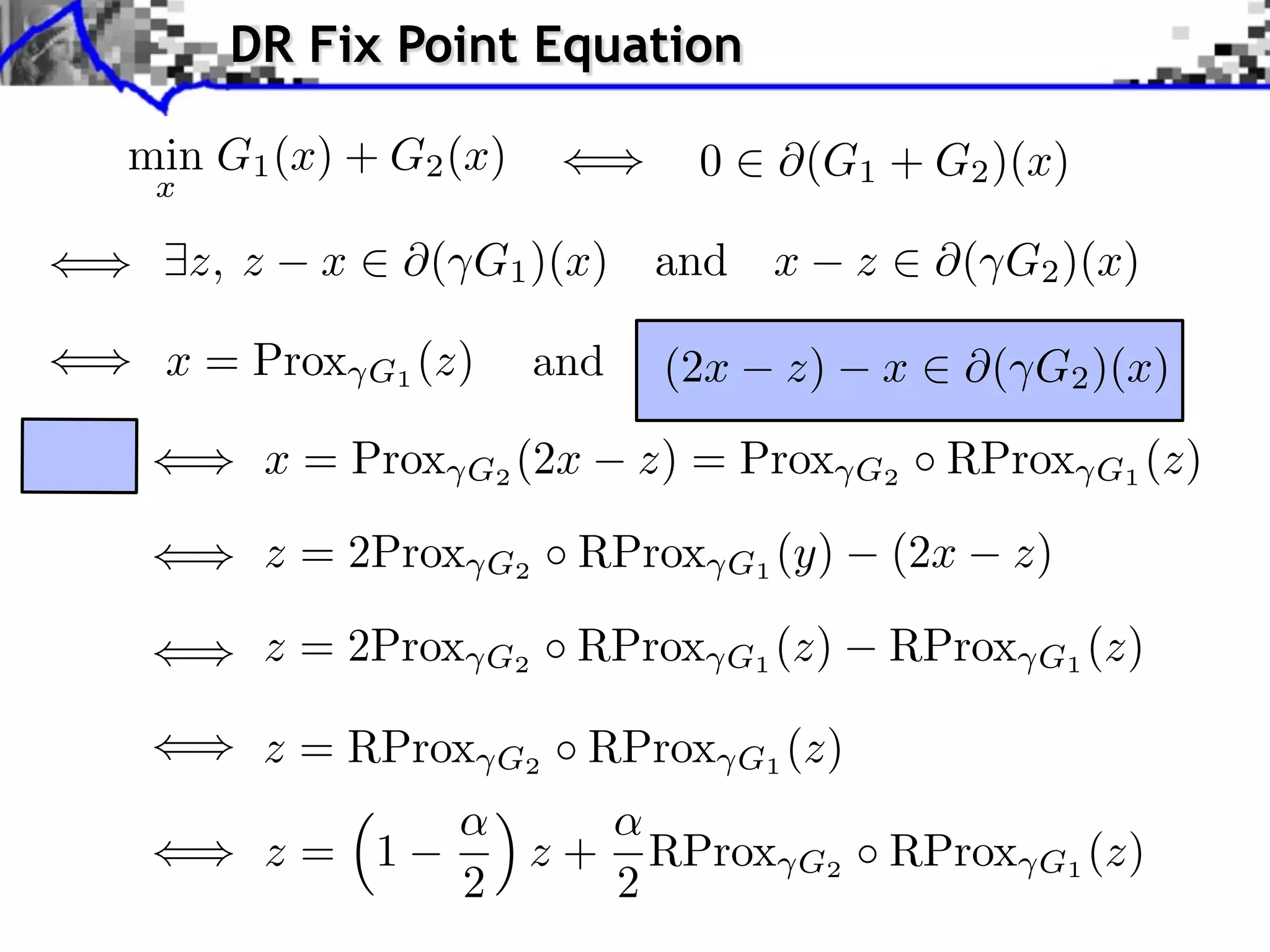
DR Fix Point Equation min G1 (x) + G2 (x) 0 (G1 + G2 )(x) x z, z x ⇥( G1 )(x) and x z ⇥( G2 )(x) x = Prox G1 (z) and (2x z) x ⇥( G2 )(x) x = Prox G2 (2x z) = Prox G2 RProx G1 (z) z = 2Prox G2 RProx G1 (y) (2x z) z = 2Prox G2 RProx G1 (z) RProx G1 (z) z = RProx G2 RProx G1 (z) z= 1 z+ RProx G2 RProx G1 (z) 2 2

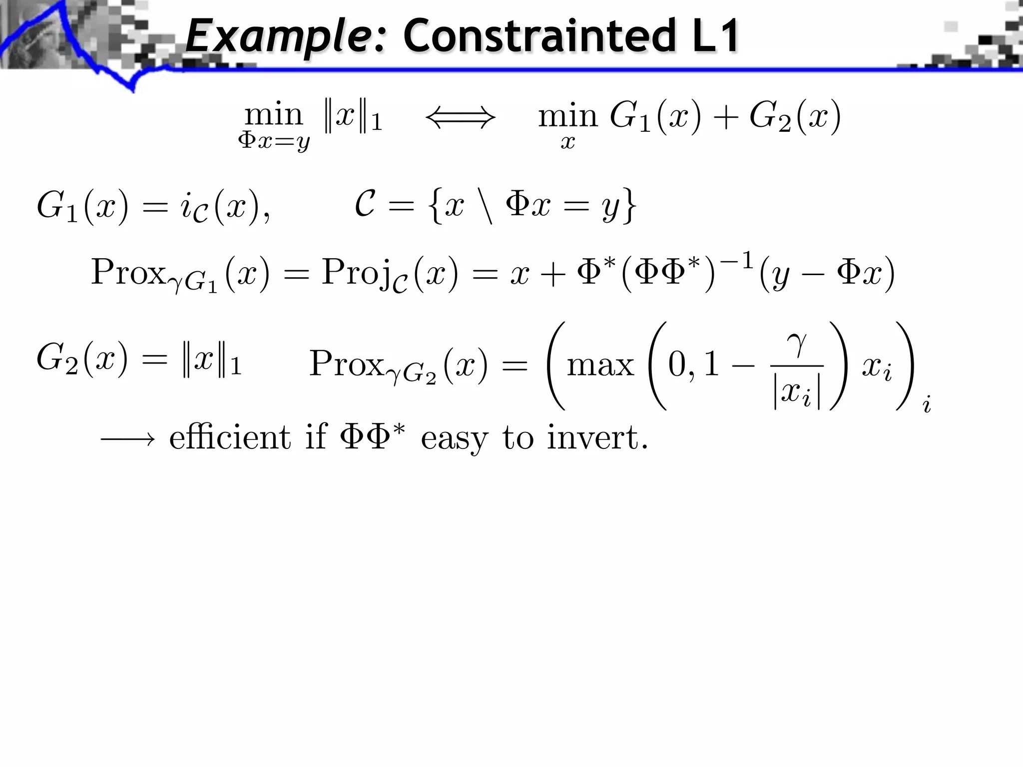
Example: Constrainted L1 min ||x||1 min G1 (x) + G2 (x) x=y x G1 (x) = iC (x), C = {x x = y} Prox G1 (x) = ProjC (x) = x + ⇥ ( ⇥ ) 1 (y x) G2 (x) = ||x||1 Prox G2 (x) = max 0, 1 xi |xi | i e⇥cient if easy to invert.

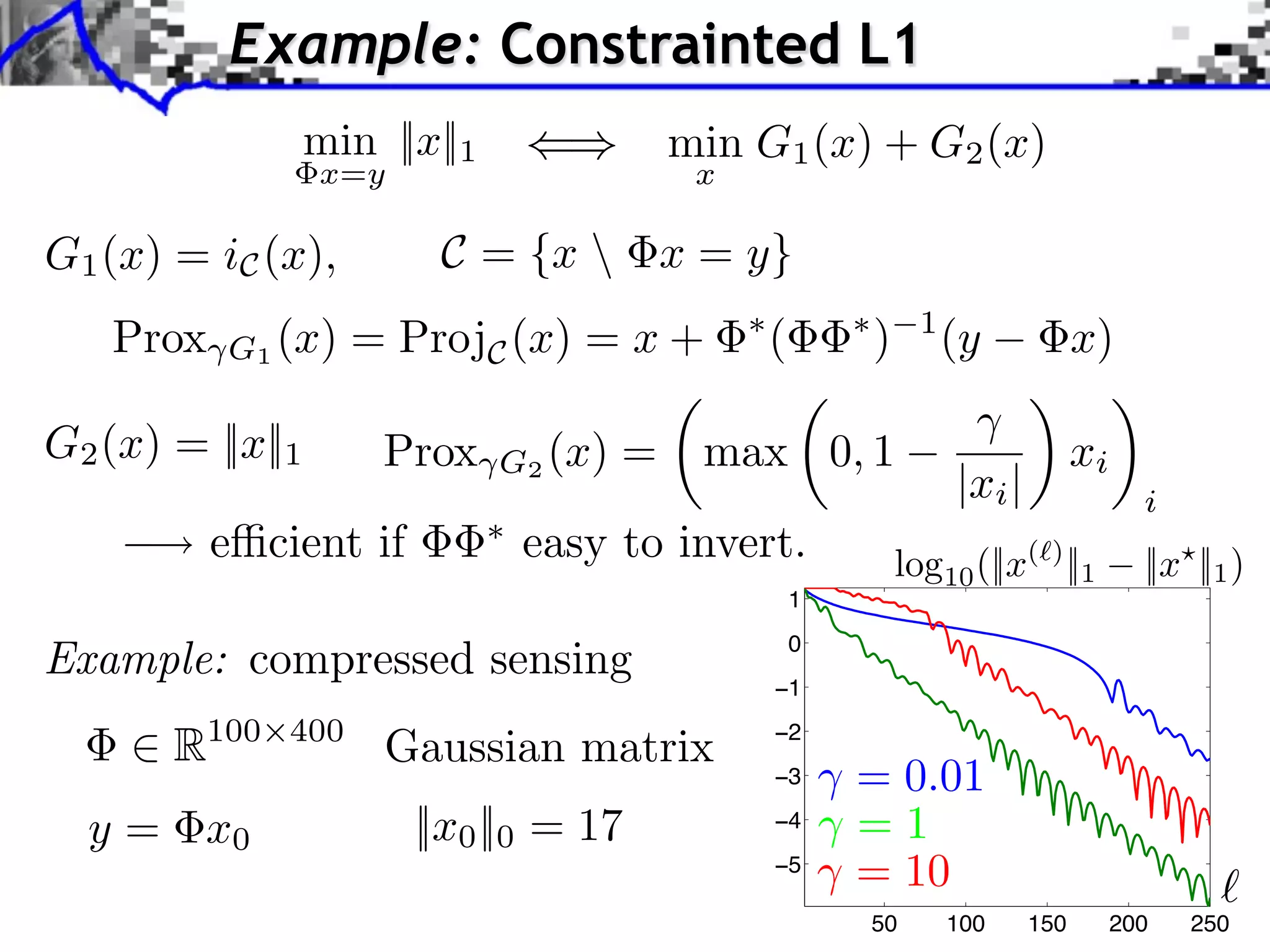
Example: Constrainted L1 min ||x||1 min G1 (x) + G2 (x) x=y x G1 (x) = iC (x), C = {x x = y} Prox G1 (x) = ProjC (x) = x + ⇥ ( ⇥ ) 1 (y x) G2 (x) = ||x||1 Prox G2 (x) = max 0, 1 xi |xi | i e⇥cient if easy to invert. log10 (||x( ) ||1 ||x ||1 ) 1 Example: compressed sensing −1 0 R100 400 Gaussian matrix −2 −3 = 0.01 y = x0 ||x0 ||0 = 17 −4 =1 −5 = 10 50 100 150 200 250

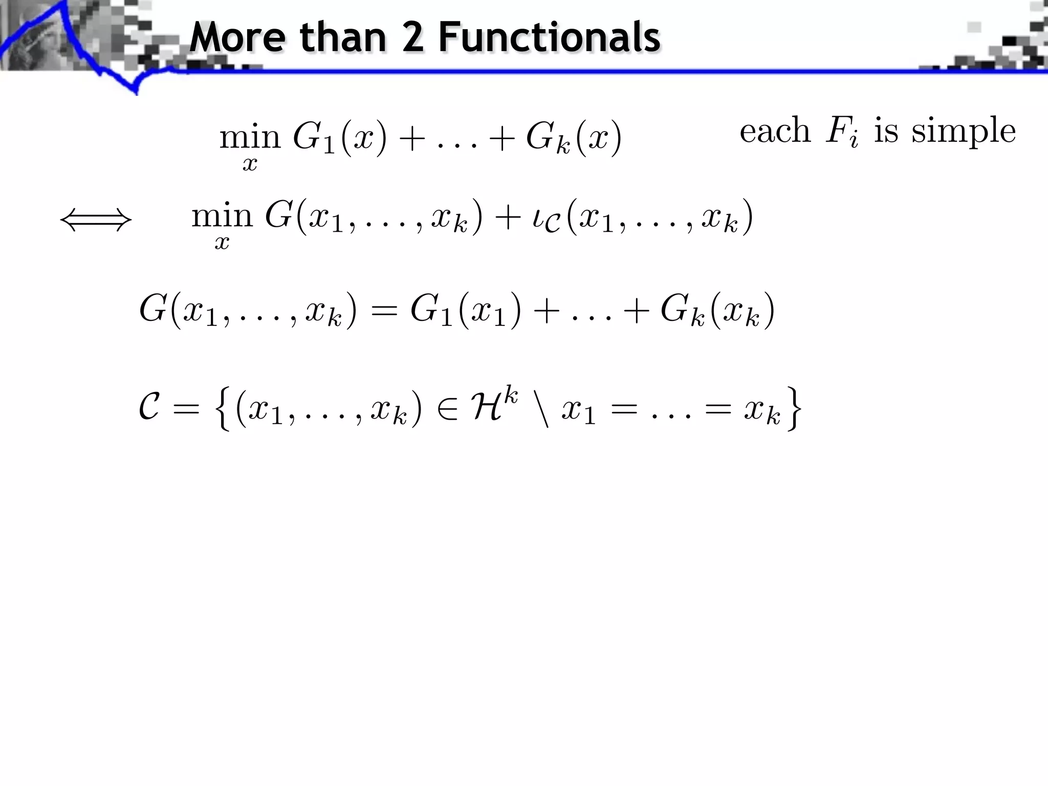
More than 2 Functionals min G1 (x) + . . . + Gk (x) each Fi is simple x min G(x1 , . . . , xk ) + C (x1 , . . . , xk ) x G(x1 , . . . , xk ) = G1 (x1 ) + . . . + Gk (xk ) C = (x1 , . . . , xk ) Hk x1 = . . . = xk

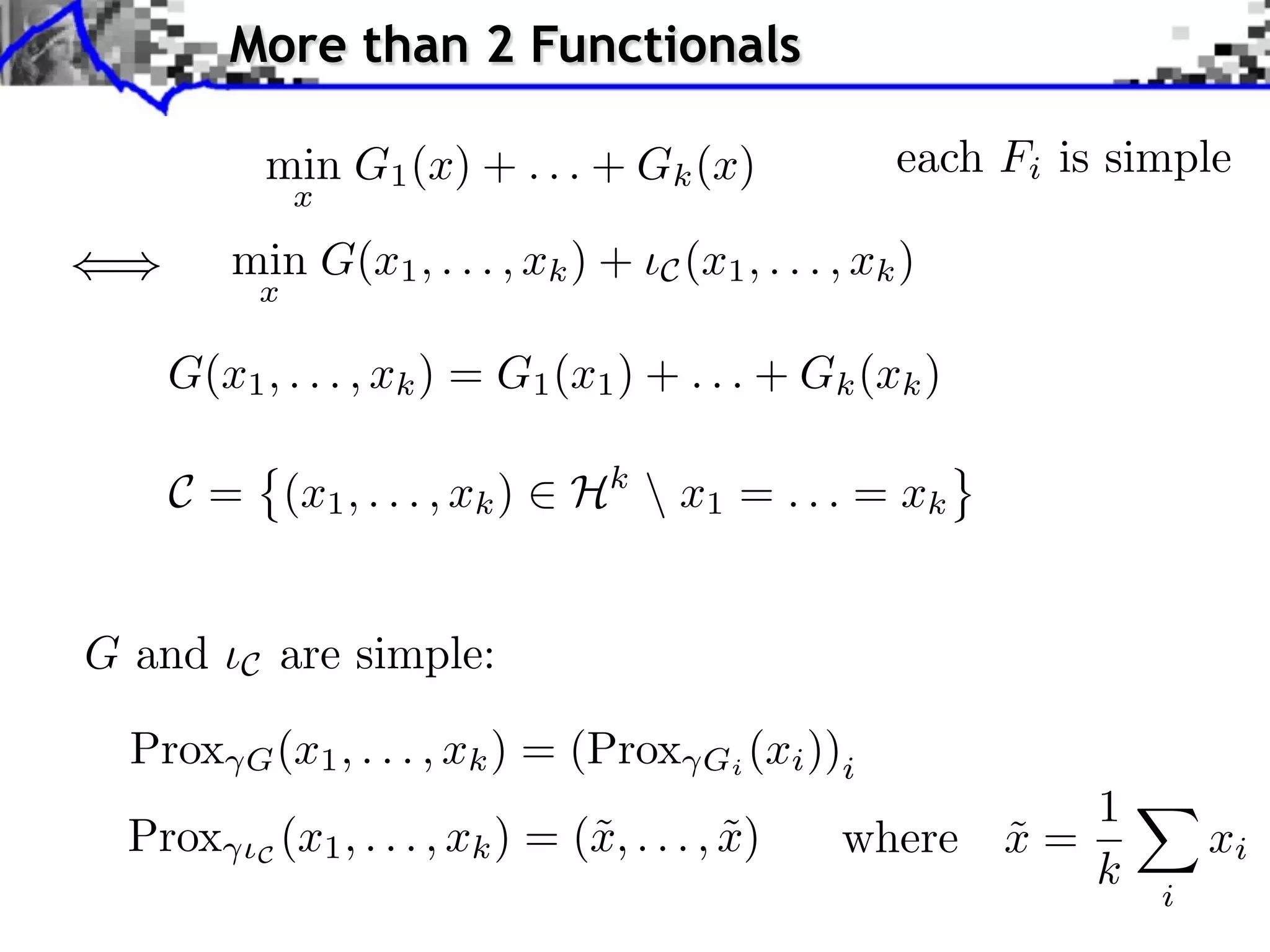
More than 2 Functionals min G1 (x) + . . . + Gk (x) each Fi is simple x min G(x1 , . . . , xk ) + C (x1 , . . . , xk ) x G(x1 , . . . , xk ) = G1 (x1 ) + . . . + Gk (xk ) C = (x1 , . . . , xk ) Hk x1 = . . . = xk G and C are simple: Prox G (x1 , . . . , xk ) = (Prox Gi (xi ))i 1 Prox ⇥C (x1 , . . . , xk ) = (˜, . . . , x) x ˜ where x = ˜ xi k i

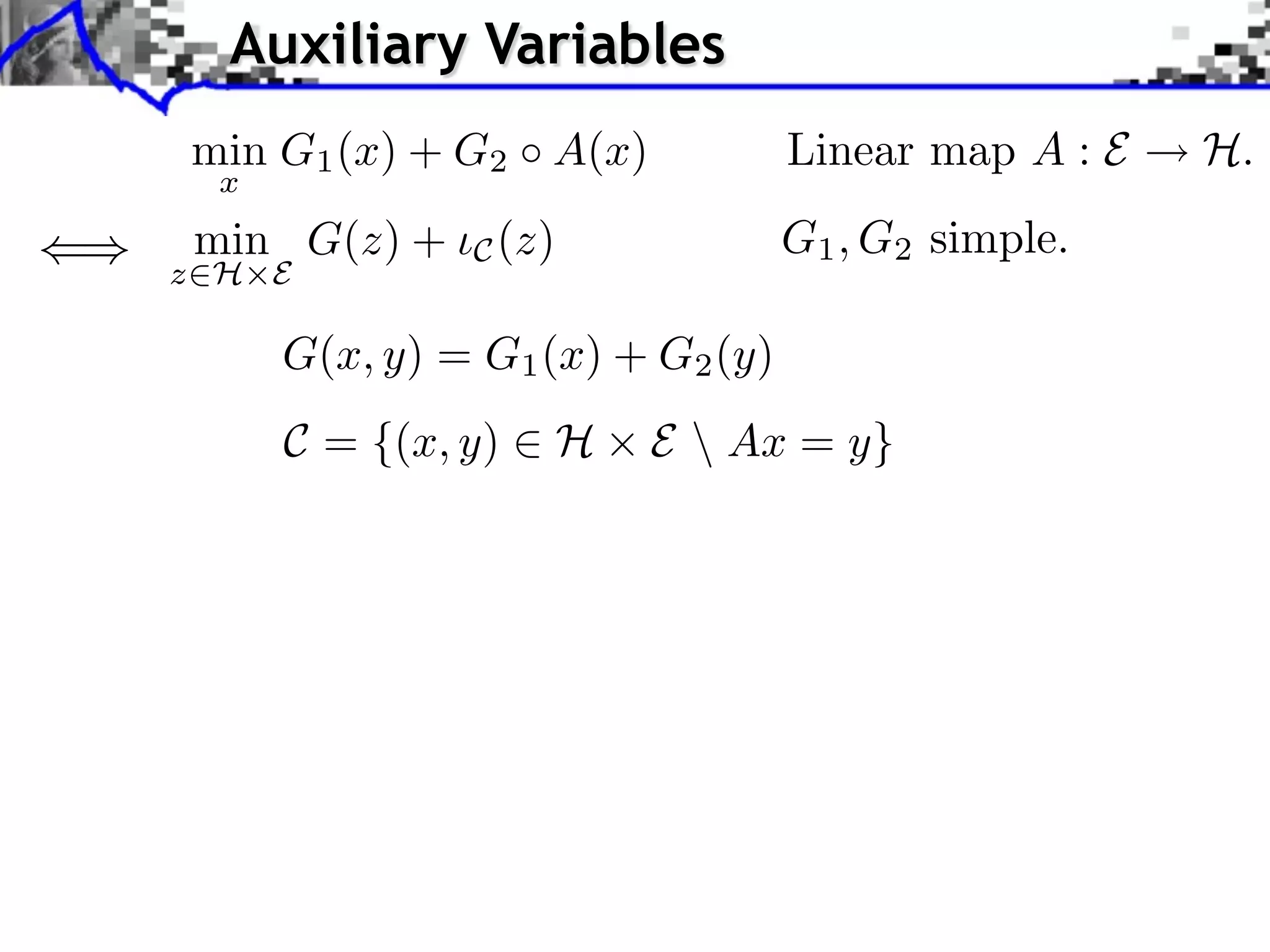
Auxiliary Variables min G1 (x) + G2 A(x) Linear map A : E H. x min G(z) + C (z) G1 , G2 simple. z⇥H E G(x, y) = G1 (x) + G2 (y) C = {(x, y) ⇥ H E Ax = y}

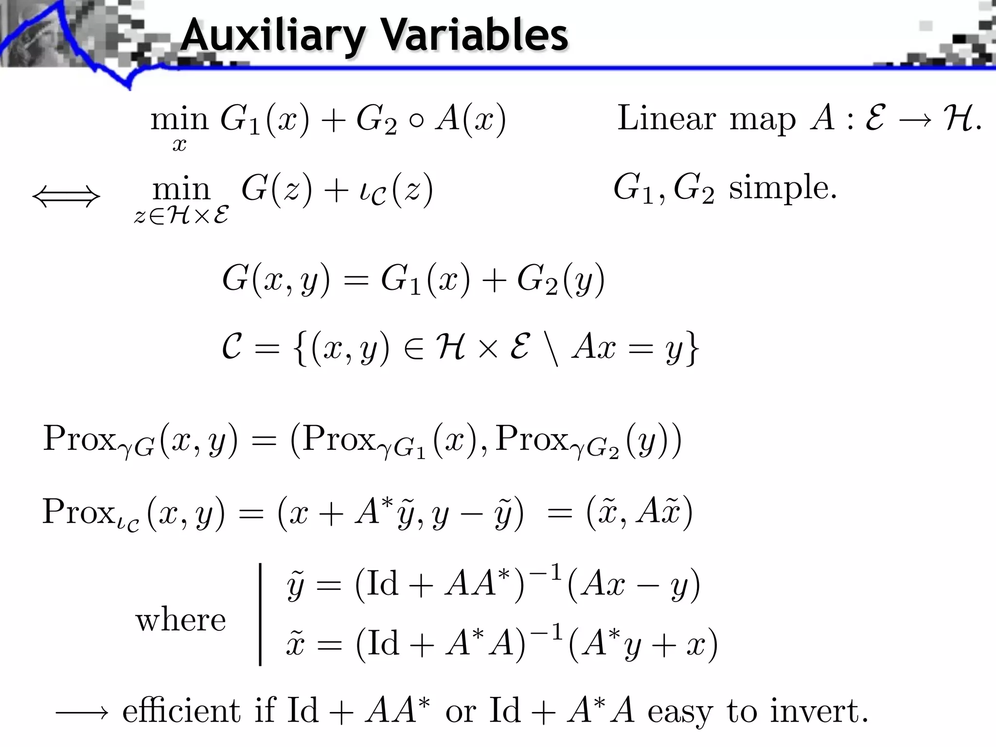
Auxiliary Variables min G1 (x) + G2 A(x) Linear map A : E H. x min G(z) + C (z) G1 , G2 simple. z⇥H E G(x, y) = G1 (x) + G2 (y) C = {(x, y) ⇥ H E Ax = y} Prox G (x, y) = (Prox G1 (x), Prox G2 (y)) Prox C (x, y) = (x + A y , y ˜ y ) = (˜, A˜) ˜ x x y = (Id + AA ) ˜ 1 (Ax y) where x = (Id + A A) ˜ 1 (A y + x) e cient if Id + AA or Id + A A easy to invert.

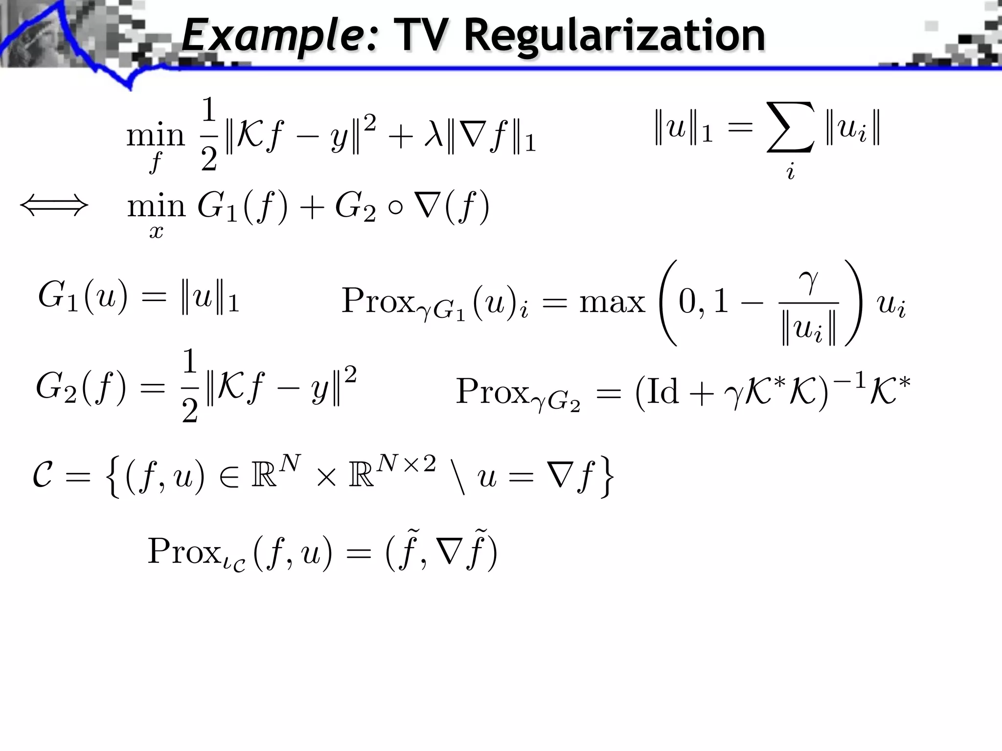
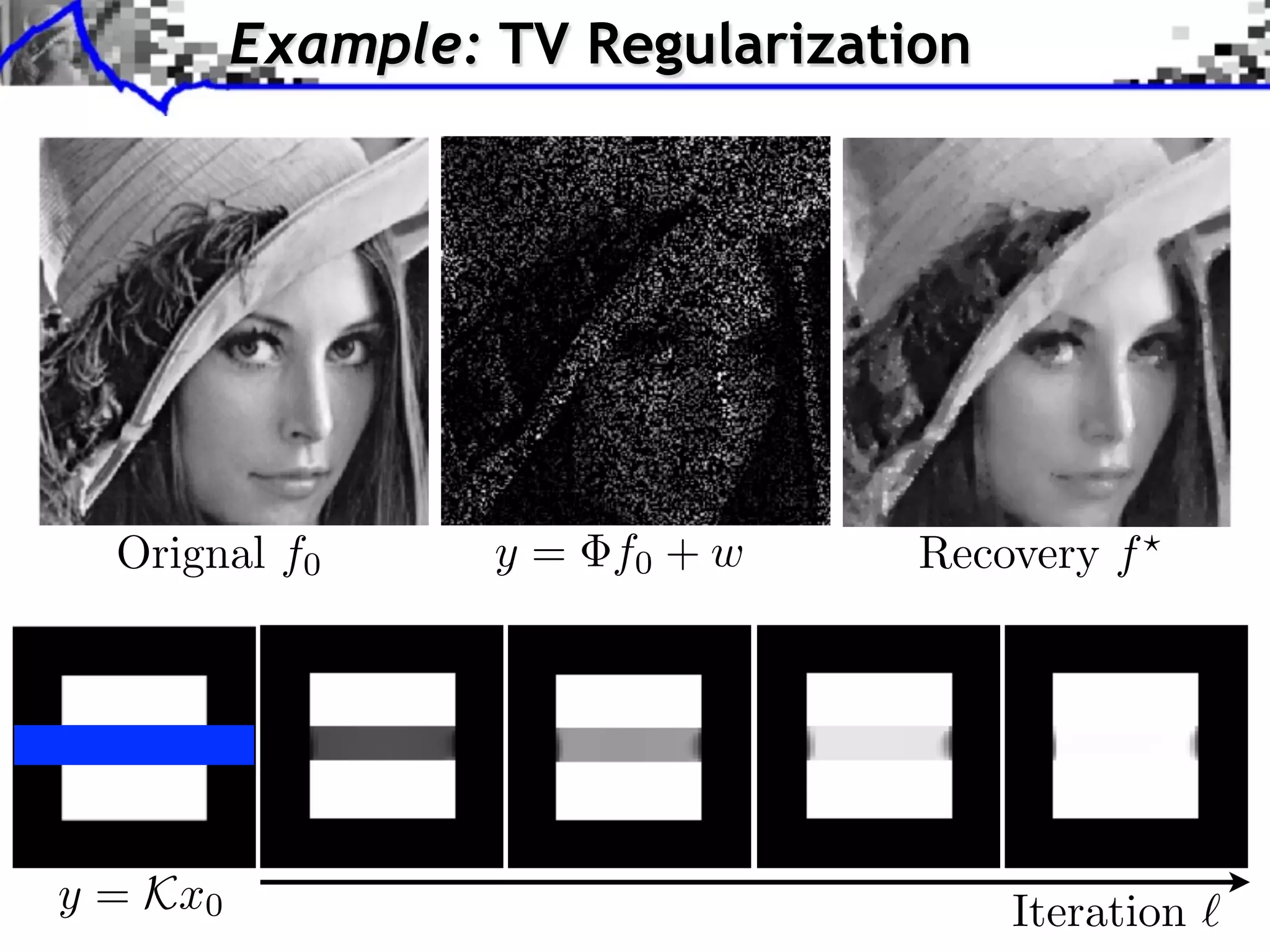
Example: TV Regularization 1 ||u||1 = ||ui || min ||Kf y||2 + ||⇥f ||1 f 2 i min G1 (f ) + G2 (f ) x G1 (u) = ||u||1 Prox G1 (u)i = max 0, 1 ui ||ui || 1 G2 (f ) = ||Kf y||2 Prox = (Id + K K) 1 K 2 G2 C = (f, u) ⇥ RN RN 2 u = ⇤f ˜ ˜ Prox C (f, u) = (f , f )

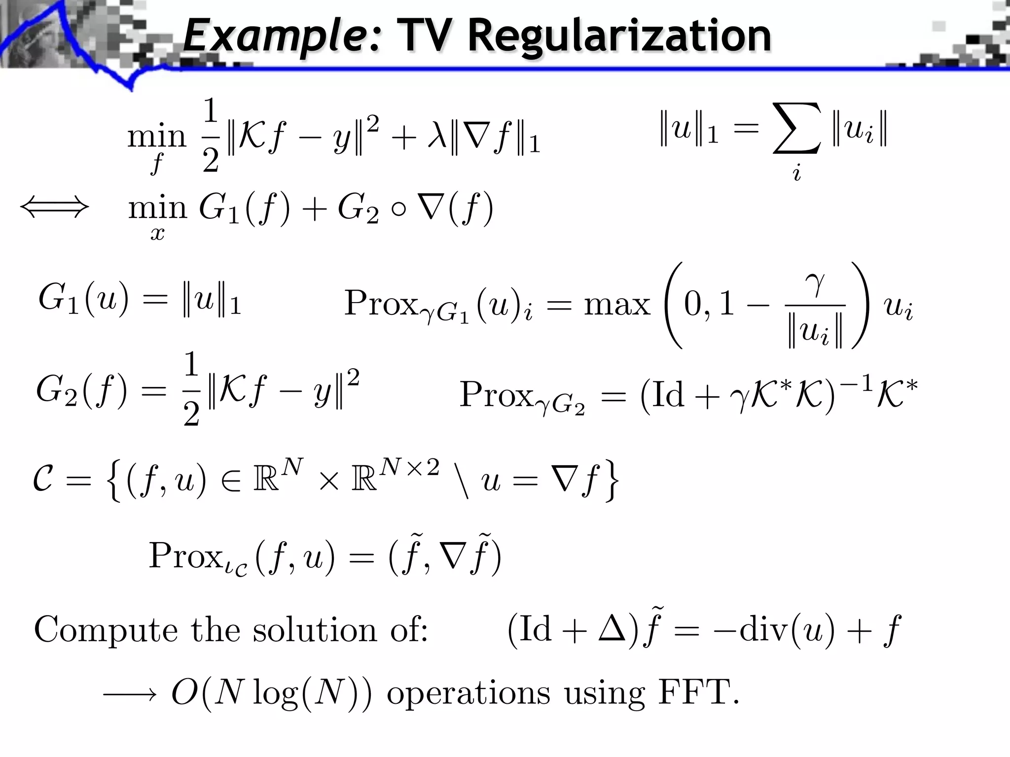
Example: TV Regularization 1 ||u||1 = ||ui || min ||Kf y||2 + ||⇥f ||1 f 2 i min G1 (f ) + G2 (f ) x G1 (u) = ||u||1 Prox G1 (u)i = max 0, 1 ui ||ui || 1 G2 (f ) = ||Kf y||2 Prox = (Id + K K) 1 K 2 G2 C = (f, u) ⇥ RN RN 2 u = ⇤f ˜ ˜ Prox C (f, u) = (f , f ) Compute the solution of: (Id + ˜ )f = div(u) + f O(N log(N )) operations using FFT.

Example: TV Regularization Orignal f0 y = f0 + w Recovery f y = Kx0 Iteration

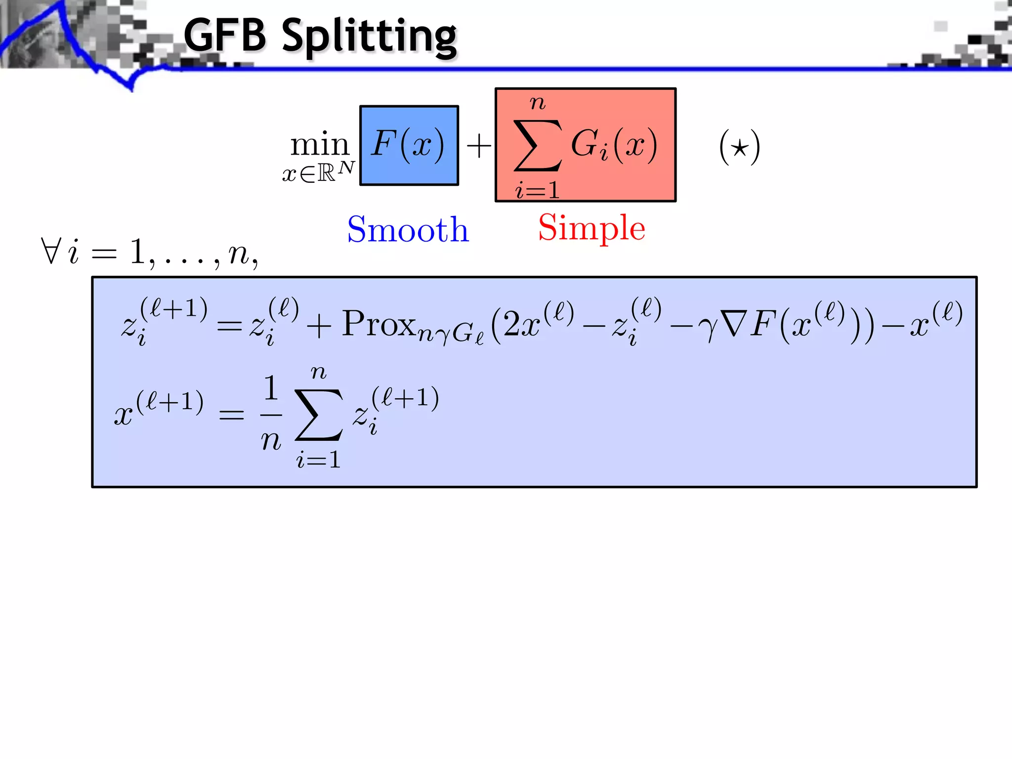
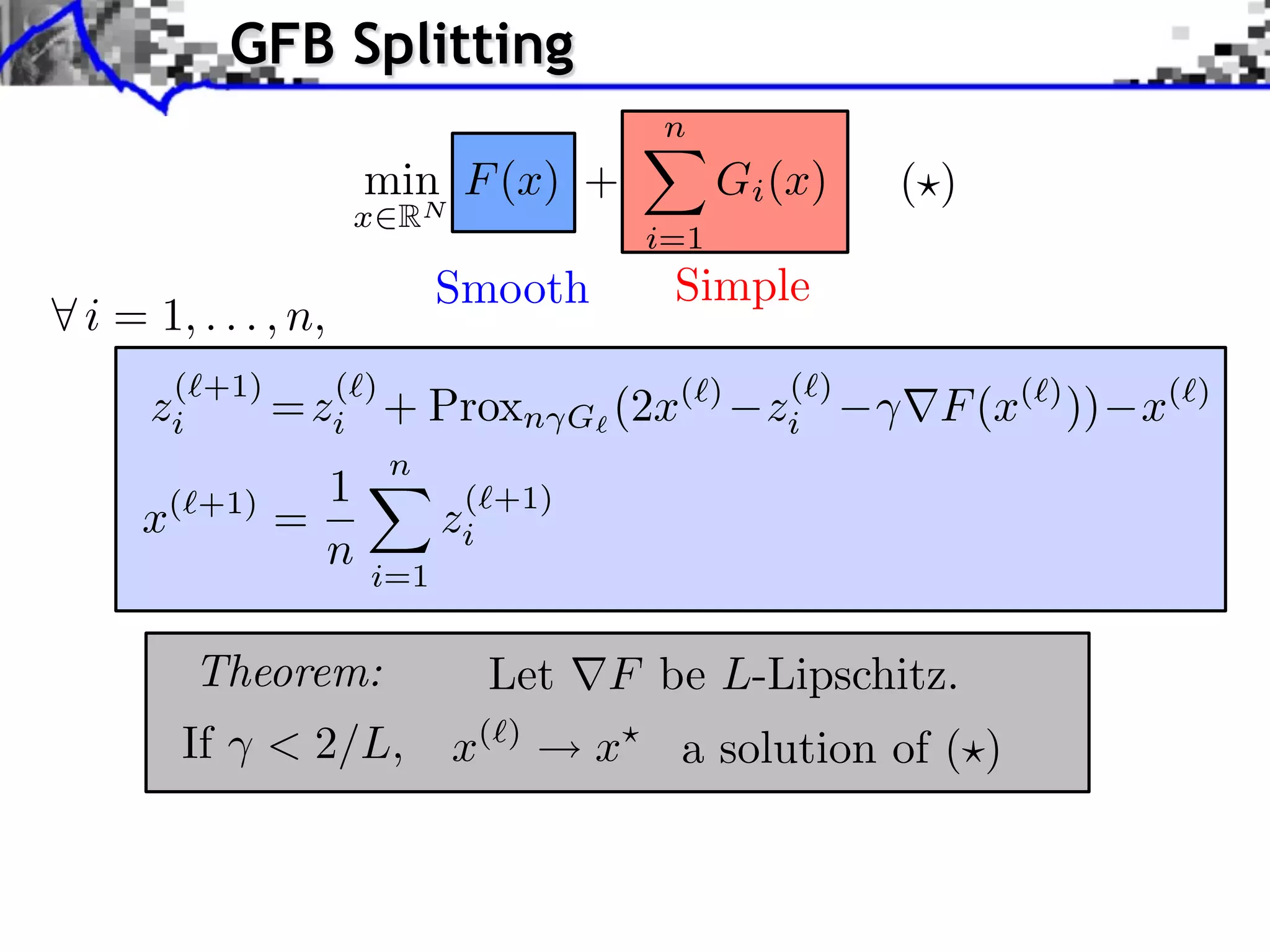
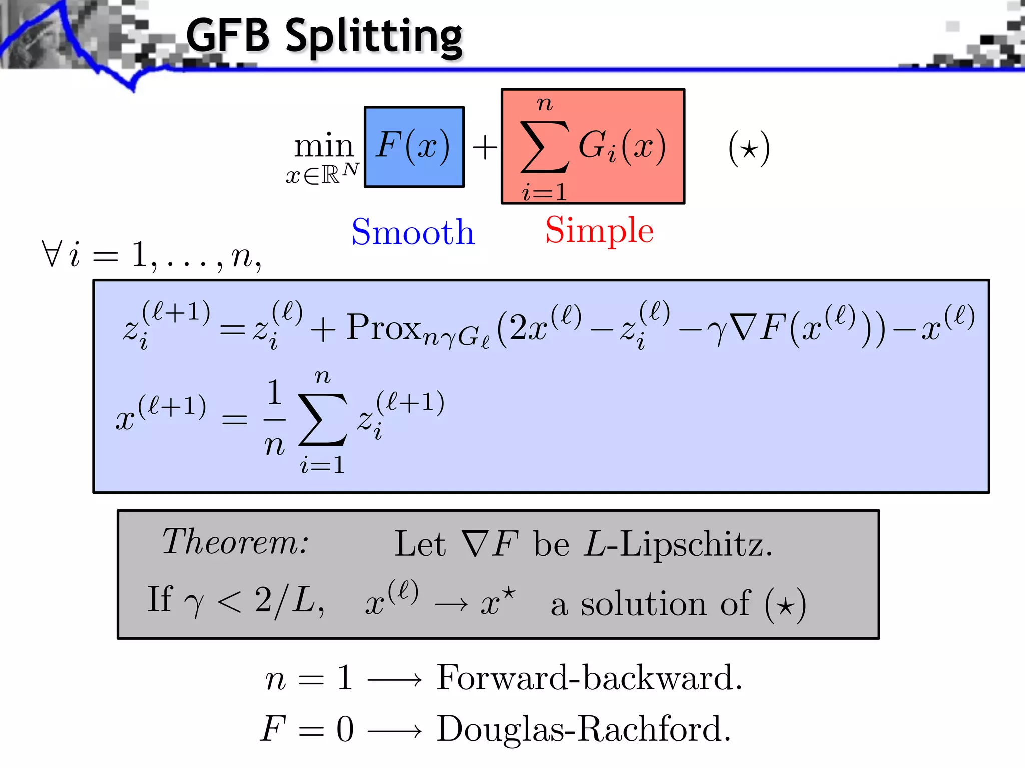
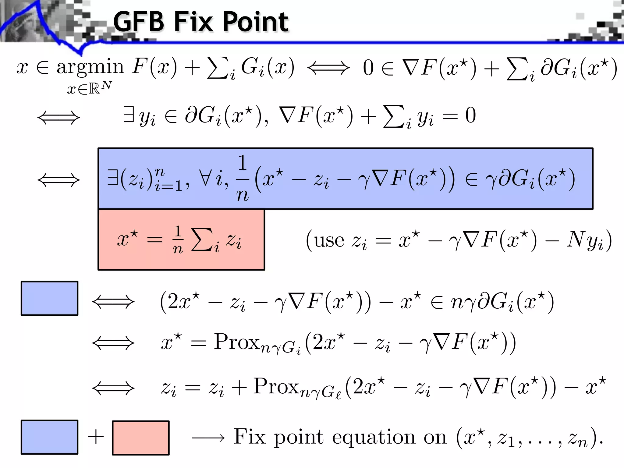
GFB Splitting n min F (x) + Gi (x) ( ) x RN i=1 Smooth Simple i = 1, . . . , n, (⇥+1) (⇥) (⇥) zi = zi + Proxn G (2x (⇥) zi F (x(⇥) )) x(⇥) n 1 ( +1) x( +1) = zi n i=1

GFB Splitting n min F (x) + Gi (x) ( ) x RN i=1 Smooth Simple i = 1, . . . , n, (⇥+1) (⇥) (⇥) zi = zi + Proxn G (2x (⇥) zi F (x(⇥) )) x(⇥) n 1 ( +1) x( +1) = zi n i=1 Theorem: Let F be L-Lipschitz. If < 2/L, x( ) x a solution of ( )

GFB Splitting n min F (x) + Gi (x) ( ) x RN i=1 Smooth Simple i = 1, . . . , n, (⇥+1) (⇥) (⇥) zi = zi + Proxn G (2x (⇥) zi F (x(⇥) )) x(⇥) n 1 ( +1) x( +1) = zi n i=1 Theorem: Let F be L-Lipschitz. If < 2/L, x( ) x a solution of ( ) n=1 Forward-backward. F =0 Douglas-Rachford.

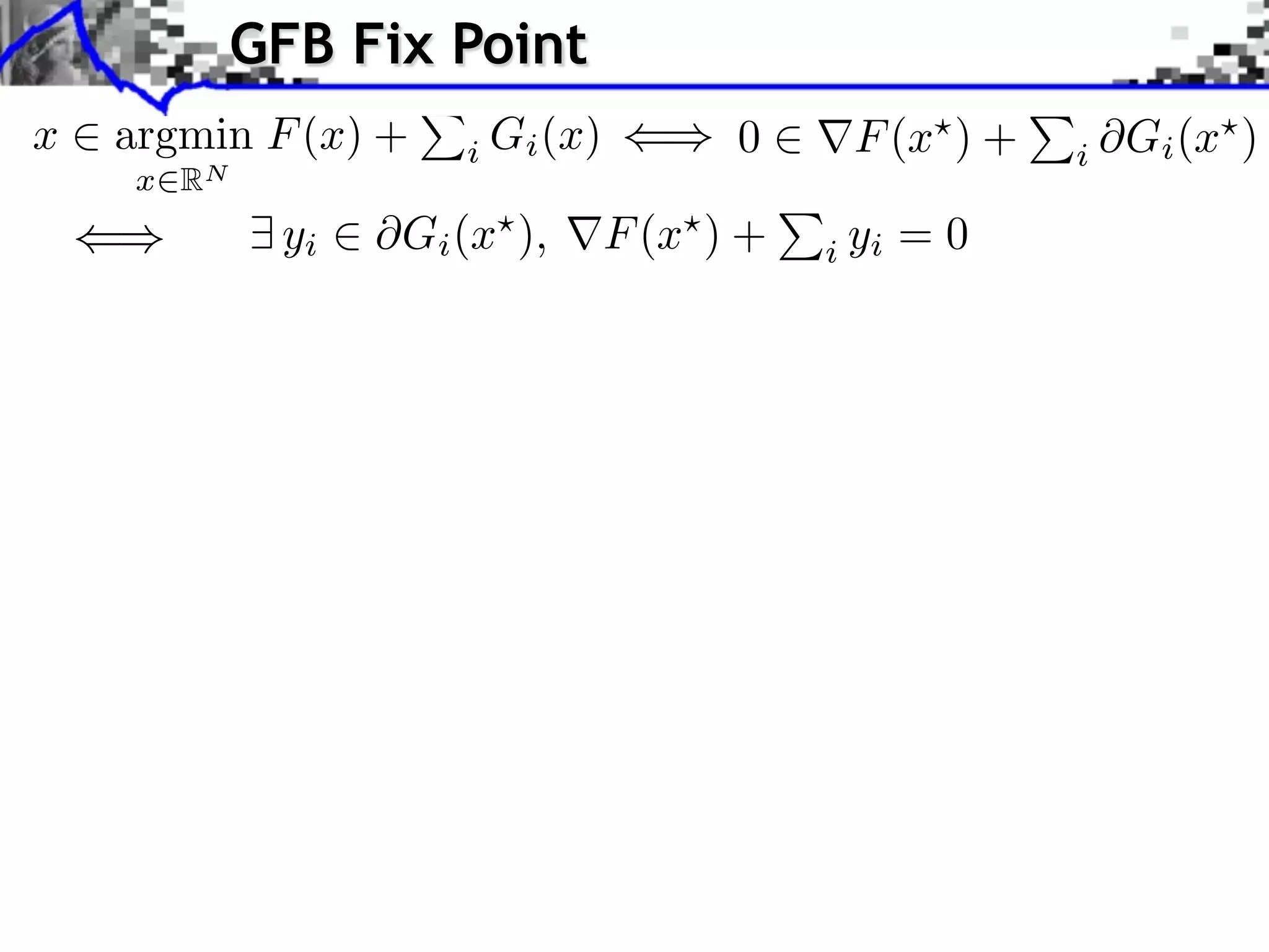
GFB Fix Point x argmin F (x) + i Gi (x) 0 F (x ) + i Gi (x ) x RN yi Gi (x ), F (x ) + i yi =0

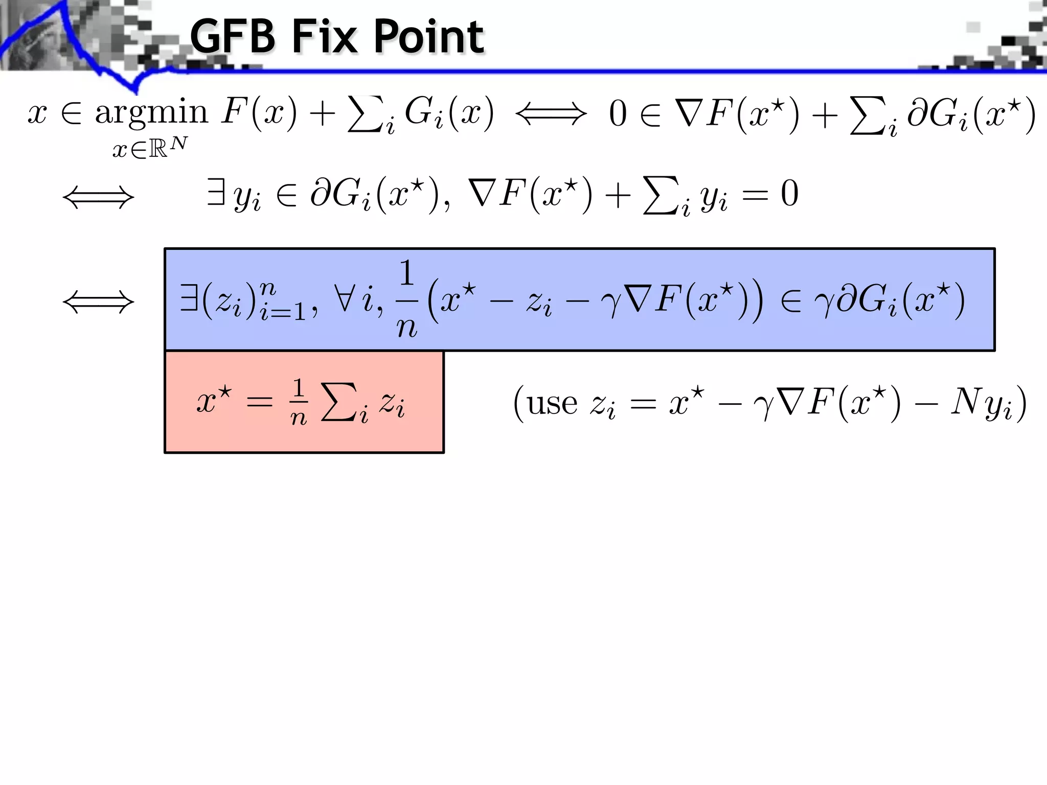
GFB Fix Point x argmin F (x) + i Gi (x) 0 F (x ) + i Gi (x ) x RN yi Gi (x ), F (x ) + i yi =0 1 (zi )n , i=1 i, x zi F (x ) ⇥Gi (x ) n x = 1 n i zi (use zi = x F (x ) N yi )

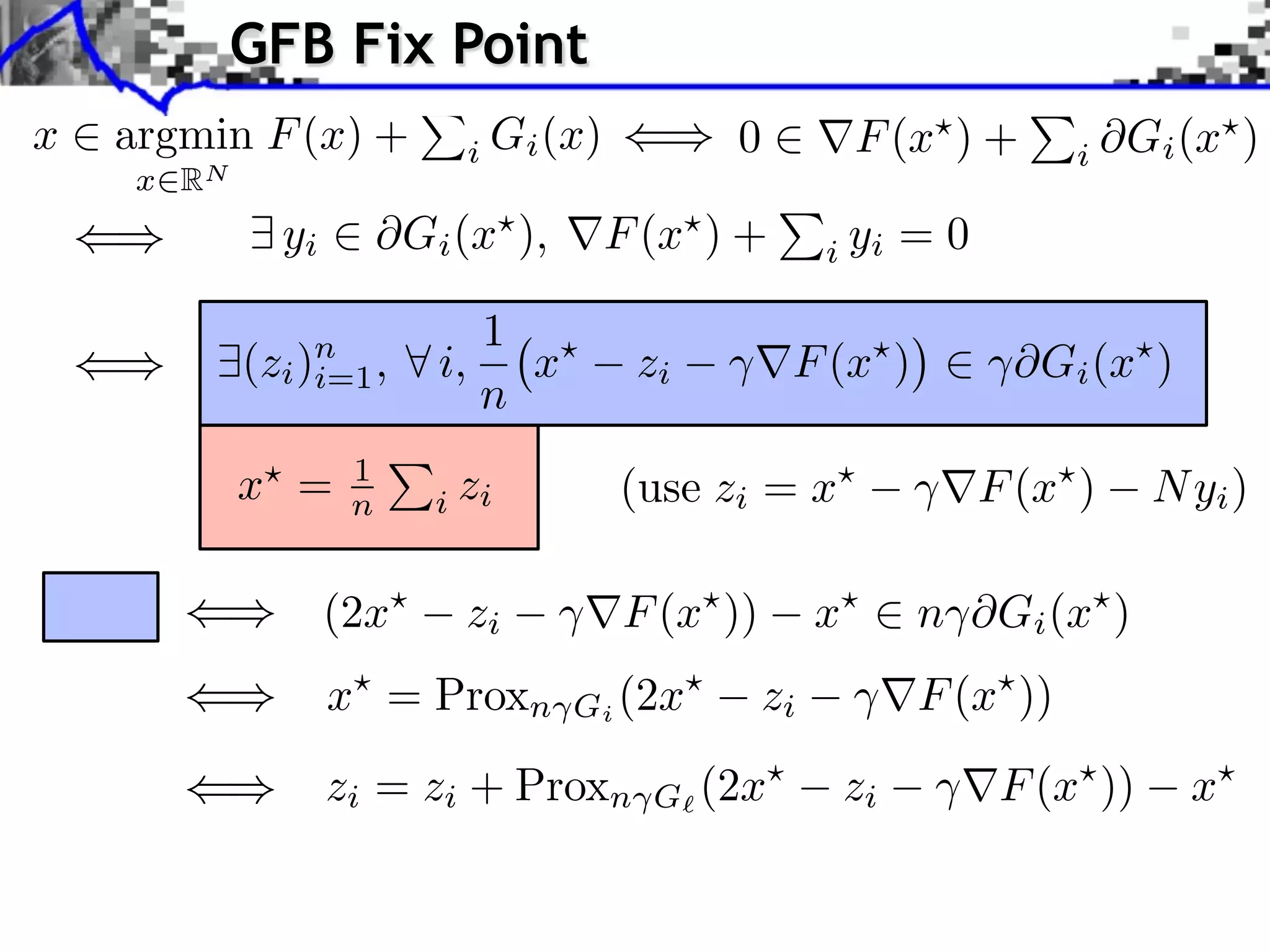
GFB Fix Point x argmin F (x) + i Gi (x) 0 F (x ) + i Gi (x ) x RN yi Gi (x ), F (x ) + i yi =0 1 (zi )n , i=1 i, x zi F (x ) ⇥Gi (x ) n x = 1 n i zi (use zi = x F (x ) N yi ) (2x zi F (x )) x n ⇥Gi (x ) x⇥ = Proxn Gi (2x⇥ zi F (x⇥ )) zi = zi + Proxn G (2x⇥ zi F (x⇥ )) x⇥

GFB Fix Point x argmin F (x) + i Gi (x) 0 F (x ) + i Gi (x ) x RN yi Gi (x ), F (x ) + i yi =0 1 (zi )n , i=1 i, x zi F (x ) ⇥Gi (x ) n x = 1 n i zi (use zi = x F (x ) N yi ) (2x zi F (x )) x n ⇥Gi (x ) x⇥ = Proxn Gi (2x⇥ zi F (x⇥ )) zi = zi + Proxn G (2x⇥ zi F (x⇥ )) x⇥ + Fix point equation on (x , z1 , . . . , zn ).

Block Regularization 1 2 block sparsity: G(x) = ||x[b] ||, ||x[b] ||2 = x2 m b B m b iments Towards More Complex Penalization (2) Bk 2 + ` 1 `2 4 k=1 x 1,2 b B1 i b xi ⇥ x⇥⇥1 = i ⇥xi ⇥ b B i b xi2 + i b xi N: 256 b B2 b B Image f = x Coe cients x.

Block Regularization 1 2 block sparsity: G(x) = ||x[b] ||, ||x[b] ||2 = x2 m b B m b iments Towards More Complex Penalization Non-overlapping decomposition: B = B ... B Towards More Complex Penalization Towards More Complex Penalization n 1 n 2 G(x) =4 x iBk (2) + ` ` k=1 G 1,2 (x) Gi (x) = ||x[b] ||, 1 2 i=1 b Bi b b 1b1 B1 i b xiixb xi 22 BB ⇥ x⇥x⇥x⇥⇥1 =i ⇥x⇥x⇥xi ⇥ ⇥= ++ + i b i ⇥ ⇥1 ⇥1 = i i ⇥i i ⇥ bb B B i Bb xii2bi2xi2 bbx i N: 256 b b 2b2 B2 i BB xi2 b2xi b b xi i b B Image f = x Coe cients x. Blocks B1 B1 B2

Block Regularization 1 2 block sparsity: G(x) = ||x[b] ||, ||x[b] ||2 = x2 m b B m b iments Towards More Complex Penalization Non-overlapping decomposition: B = B ... B Towards More Complex Penalization Towards More Complex Penalization n 1 n 2 G(x) =4 x iBk (2) + ` ` k=1 G 1,2 (x) Gi (x) = ||x[b] ||, 1 2 i=1 b Bi Each Gi is simple: b b 1b1 B1 i b xiixb xi BB 22 ⇥ x⇥x⇥x⇥⇥1 =i ⇥xG ⇥xi ⇥ m = b B B i b xii2bi2xi2 ⇥ ⇥1 = i ⇥i i x + i b i ⇤ m ⇥ b ⇥ Bi , ⇥ ⇥1Prox i ⇥xi ⇥(x) b max i0, 1 = Bb bx ++m N: 256 ||x[b]b||B xi2 b2xi 2 2 B2 b B b i b b xi i b B Image f = x Coe cients x. Blocks B1 B1 B2

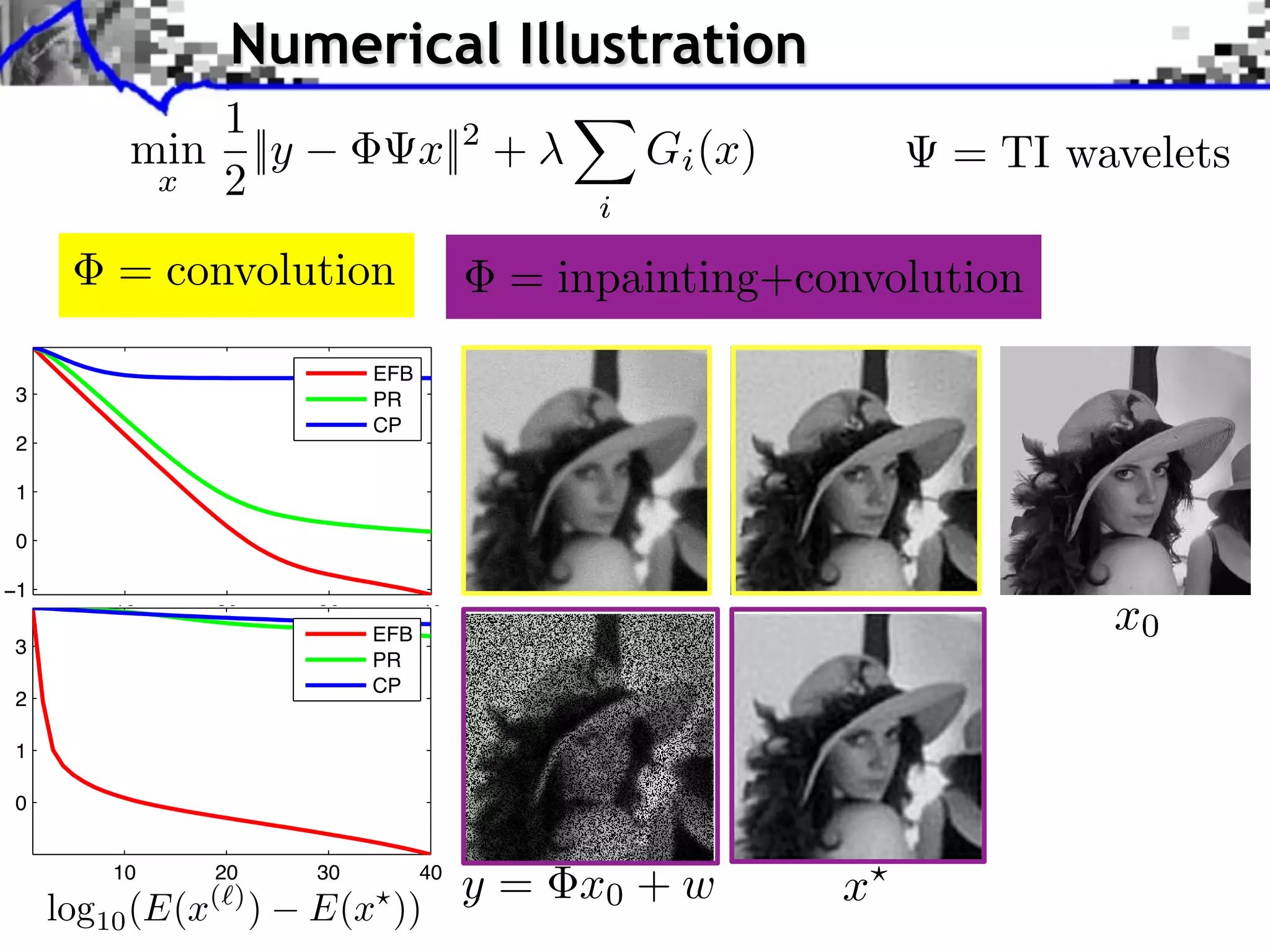
Deconv. + Inpaint. 2min+CP Y ⇥ P K x CP Y + P 1 K2 Deconv. x 2Inpaint. min 2 ⇥ ` ` x x k=1 x+1,2` k=1 log10(E−E 2 1 `2 Numerical Illustration log10(E− 1 Numerical Experiments Experiments 1 Numerical 1 TI (2)`2 4 0 ||y x 1 ⇥x||368s PRx 2 minix(x)Y ⇥ K x= + `wavelets x Bk 2 0 : 283s; tPR: 298s; tCP:: 283s; t : 298s; t (2) Deconvolution min 2 Y ⇥ K tmin −1 EFB x 102 Deconvolution +GCP: 1` 4 −1 tEFB 2 + 10 40 20 368s 30 1 2 2 40k=1 ` x 1,2 1 k=1 20 30 3 iteration 3 # i EFB iteration # EFB log10(E−Emin) log10(E−Emin) PR PR 2 = convolution 2 = inpainting+convolution l1/l2 l1/l2 : 1.30e−03; CPλ2 : 1.30e−03; CP 2 λ tPR: 173s; tCP 190s noise: 0.025; convol.::it. #50; SNR: 22.49dB #50; SNR: 22.49dB tEFB: 161s; tPR: 173s; tCP N: 256 tEFB: 161s; noise: 0.025; :convol.: 2 190s 1 Numerical Experiments 2 1 EFB it. N: 256 EFB (4) Bk Y ⇥P K + 0 0 log10(E−Emin) 3 3 1 PR 2 PR 16 onv. + Inpaint. minx 2 CP 2 30 2 x CP `140`2 k=1 x 1,2 10 20 10 40 20 30 1 iteration # 1 iteration # 0 0 λ4 : 1.00e−03; λ4 : 1.00e−03; l1/l2 l1/l2 tEFB: 283s; tPR: 298s; tCP: 368s −1 noise: 0.025; degrad.: 0.4; 0.025; degrad.: 0.4; convol.: 2 noise: convol.: 2 −1 it. #50; SNR: 21.80dB #50; SNR: 21.80dB it. 10 20 iteration # 30 EFB 40 10 20 iteration # 30 40 x0 3 PR min 2 CP λ2 : 1.30e−03; λ2 : 1.30e−03; l1/l2 l1/l2 1 noise: 0.025; convol.: 2 noise: 0.025; it. #50; SNR: 22.49dB convol.: 2 it. #50; SNR: 22.49dB 10 0 log10 10 20 (E(x( ) ) # iteration 30 E(x )) y = x0 + w 40 x 4

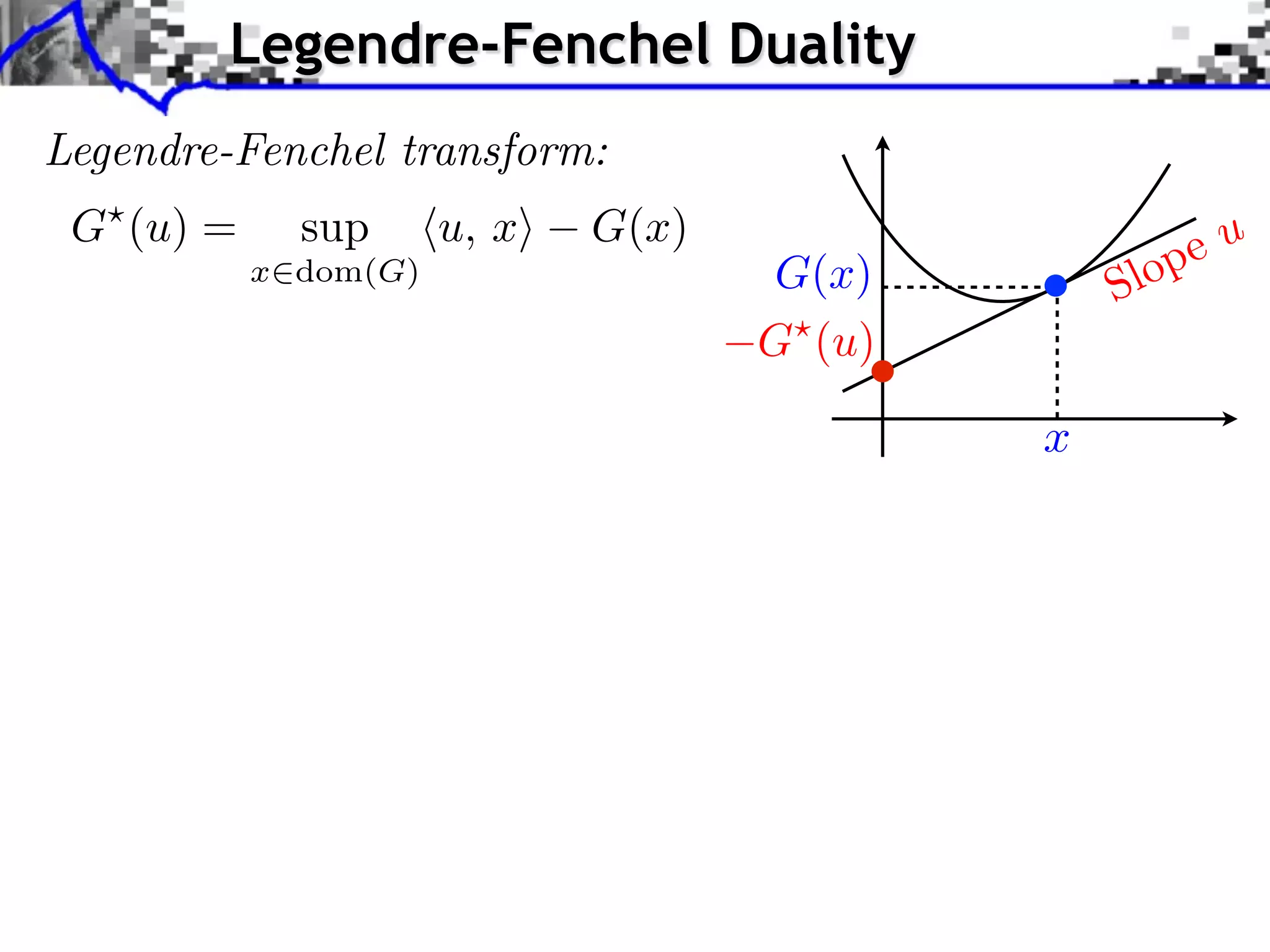
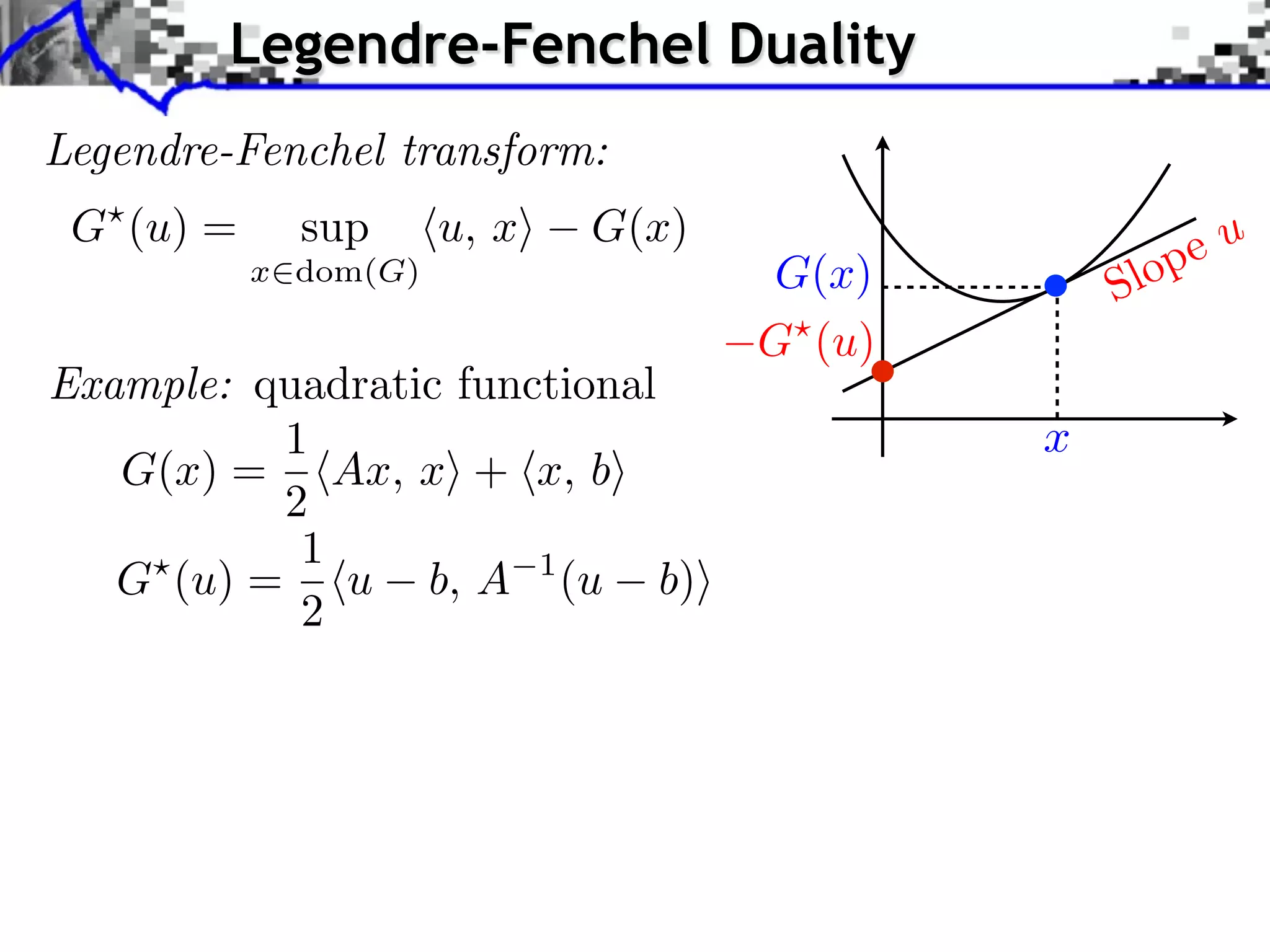
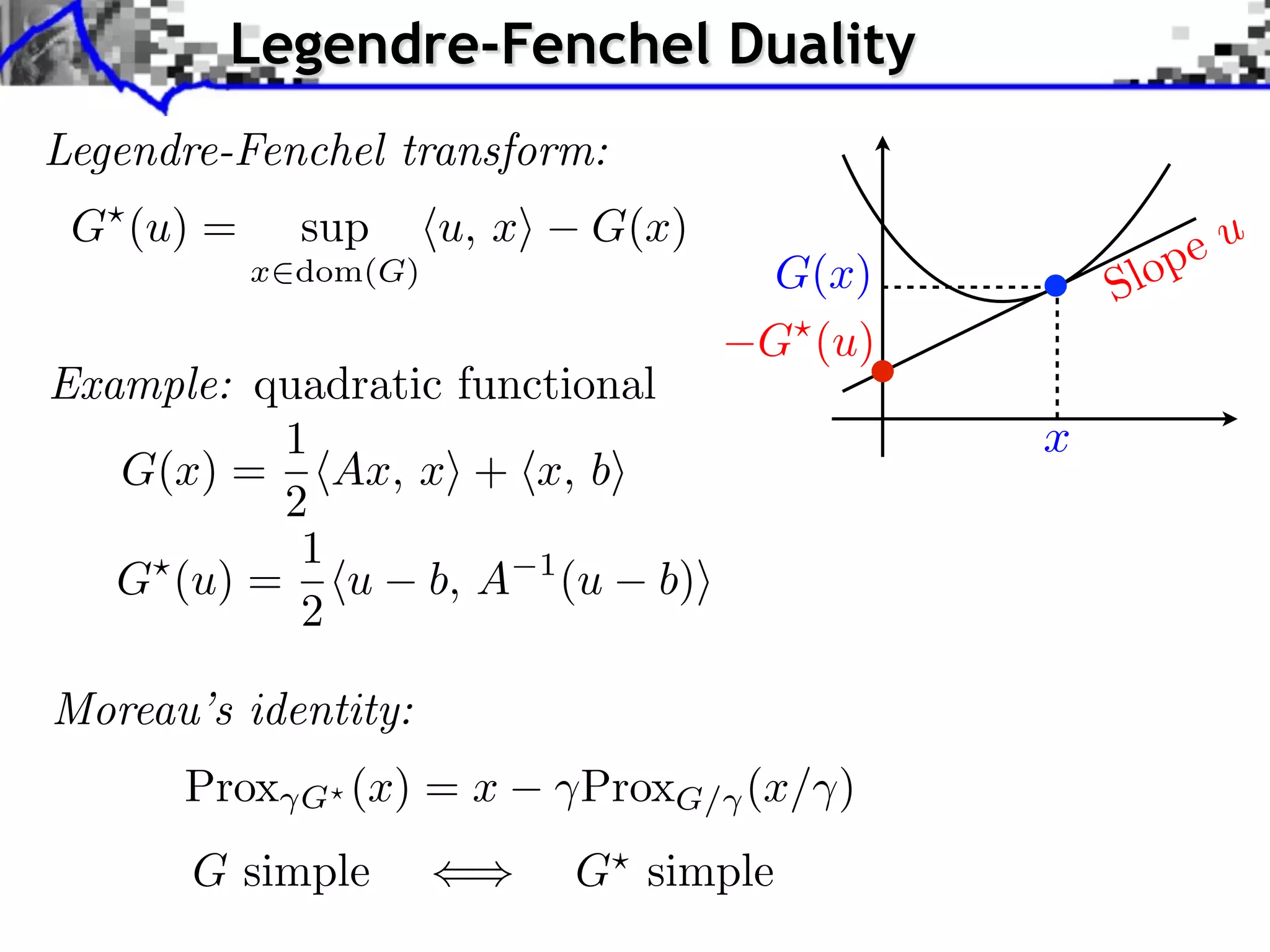
Legendre-Fenchel Duality Legendre-Fenchel transform: G (u) = sup u, x G(x) eu x dom(G) G(x) S lop G (u) x

Legendre-Fenchel Duality Legendre-Fenchel transform: G (u) = sup u, x G(x) eu x dom(G) G(x) S lop G (u) Example: quadratic functional 1 x G(x) = Ax, x + x, b 2 1 G (u) = u b, A 1 (u b) 2

Legendre-Fenchel Duality Legendre-Fenchel transform: G (u) = sup u, x G(x) eu x dom(G) G(x) S lop G (u) Example: quadratic functional 1 x G(x) = Ax, x + x, b 2 1 G (u) = u b, A 1 (u b) 2 Moreau’s identity: Prox G (x) = x ProxG/ (x/ ) G simple G simple

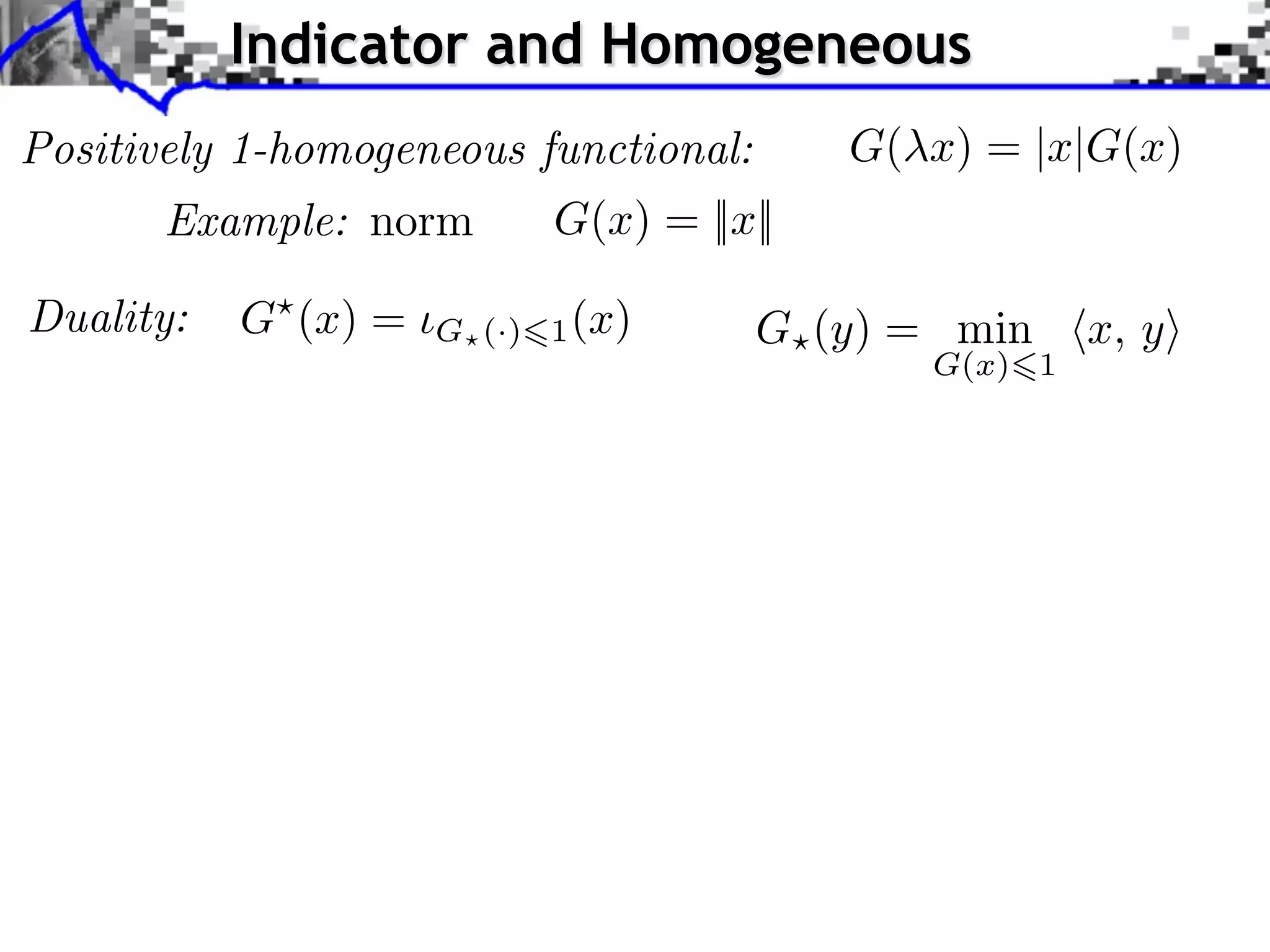
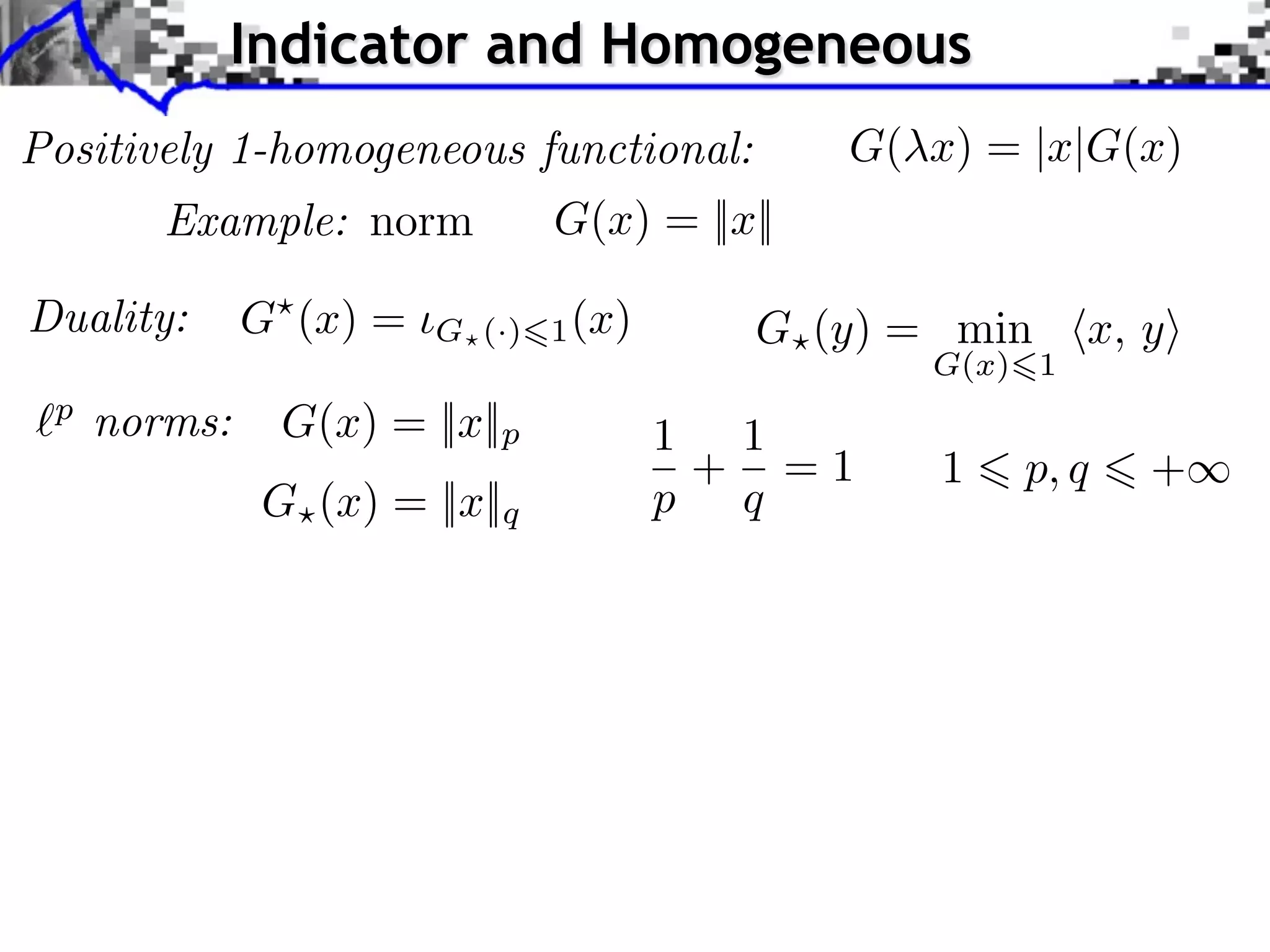
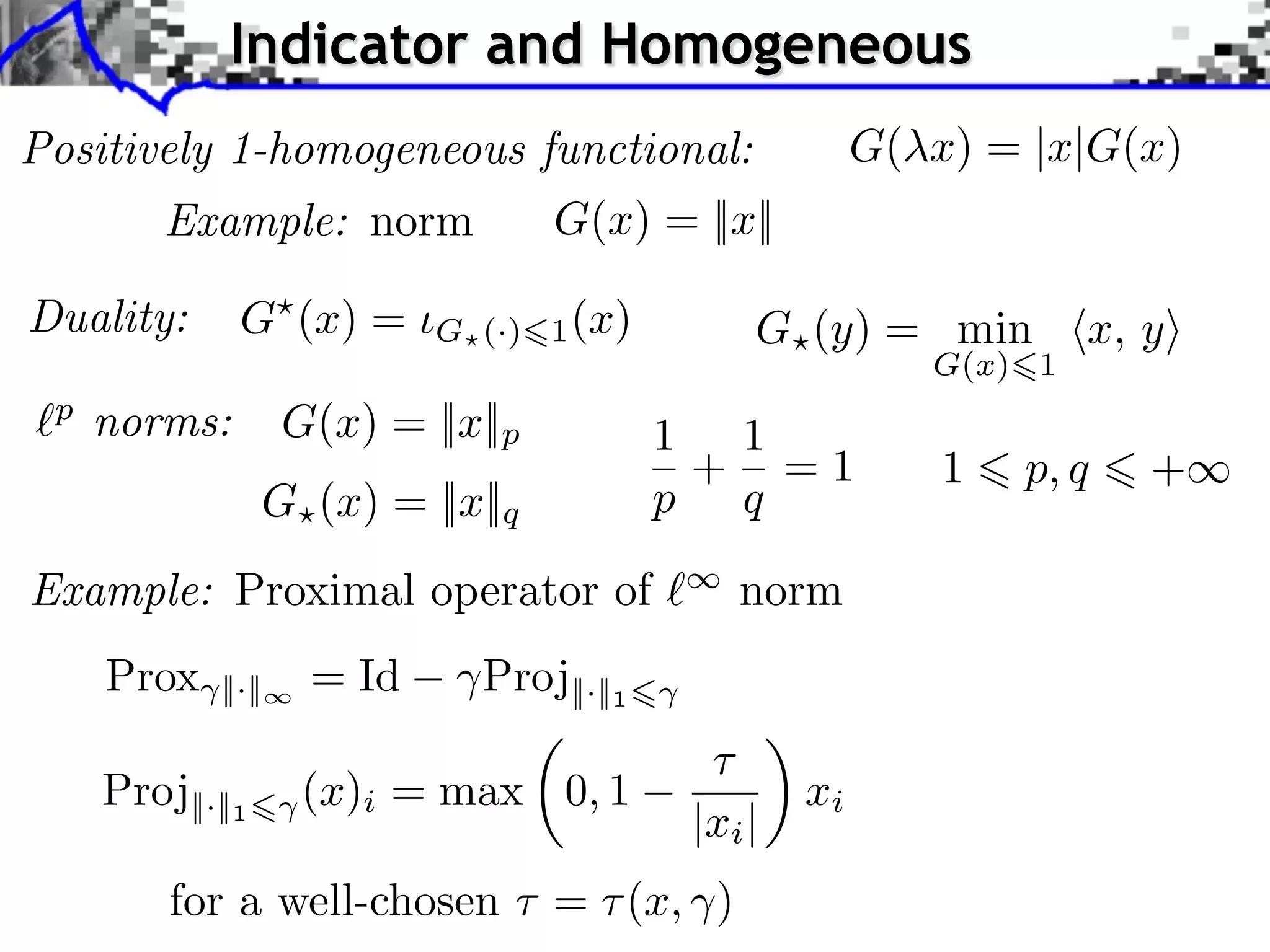
Indicator and Homogeneous Positively 1-homogeneous functional: G( x) = |x|G(x) Example: norm G(x) = ||x|| Duality: G (x) = G (·) 1 (x) G (y) = min x, y G(x) 1

Indicator and Homogeneous Positively 1-homogeneous functional: G( x) = |x|G(x) Example: norm G(x) = ||x|| Duality: G (x) = G (·) 1 (x) G (y) = min x, y G(x) 1 p norms: G(x) = ||x||p 1 1 + =1 1 p, q + G (x) = ||x||q p q

Indicator and Homogeneous Positively 1-homogeneous functional: G( x) = |x|G(x) Example: norm G(x) = ||x|| Duality: G (x) = G (·) 1 (x) G (y) = min x, y G(x) 1 p norms: G(x) = ||x||p 1 1 + =1 1 p, q + G (x) = ||x||q p q Example: Proximal operator of norm Prox ||·|| = Id Proj||·||1 Proj||·||1 (x)i = max 0, 1 xi |xi | for a well-chosen ⇥ = ⇥ (x, )

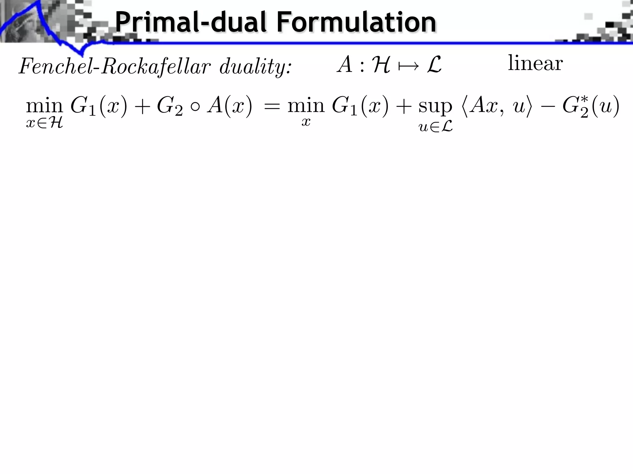
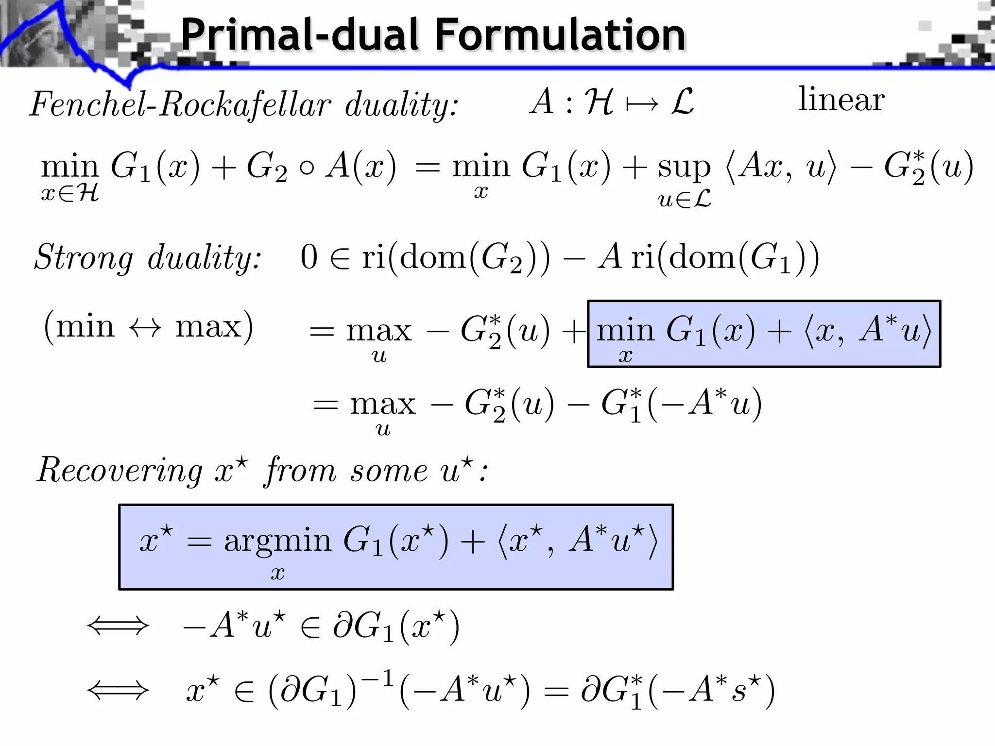
Primal-dual Formulation Fenchel-Rockafellar duality: A:H⇥ L linear min G1 (x) + G2 A(x) = min G1 (x) + sup hAx, ui G⇤ (u) 2 x2H x u2L

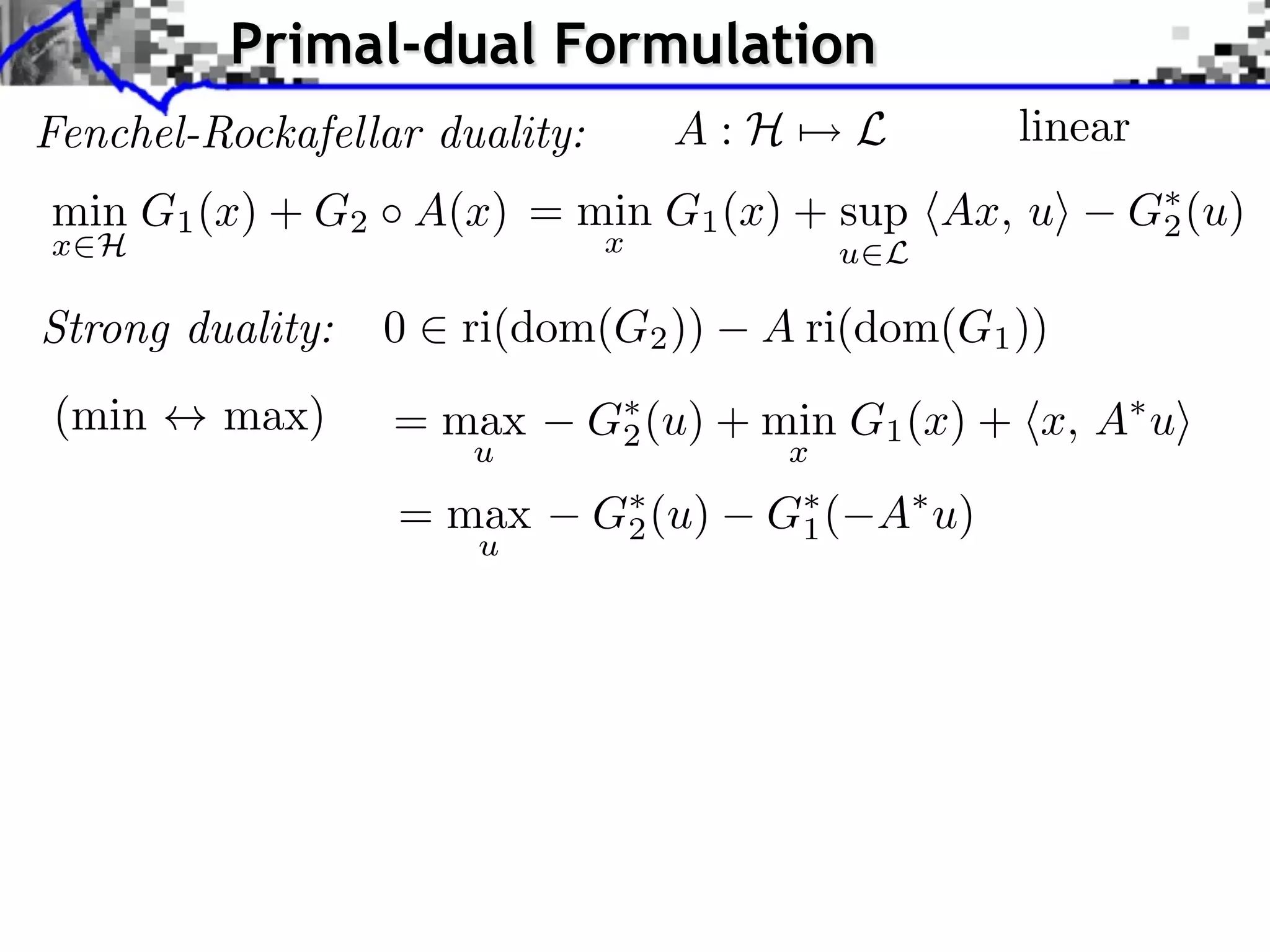
Primal-dual Formulation Fenchel-Rockafellar duality: A:H⇥ L linear min G1 (x) + G2 A(x) = min G1 (x) + sup hAx, ui G⇤ (u) 2 x2H x u2L Strong duality: 0 2 ri(dom(G2 )) A ri(dom(G1 )) (min $ max) = max G⇤ (u) + min G1 (x) + hx, A⇤ ui 2 u x = max G⇤ (u) 2 G⇤ ( 1 A⇤ u) u

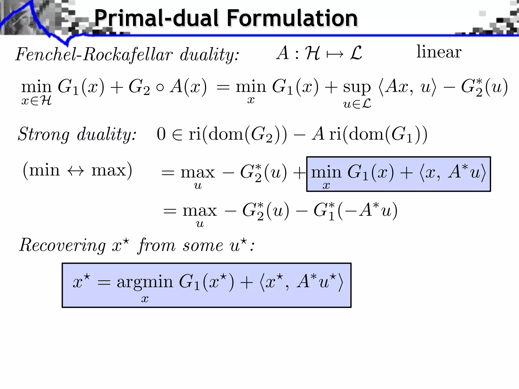
Primal-dual Formulation Fenchel-Rockafellar duality: A:H⇥ L linear min G1 (x) + G2 A(x) = min G1 (x) + sup hAx, ui G⇤ (u) 2 x2H x u2L Strong duality: 0 2 ri(dom(G2 )) A ri(dom(G1 )) (min $ max) = max G⇤ (u) + min G1 (x) + hx, A⇤ ui 2 u x = max G⇤ (u) 2 G⇤ ( 1 A⇤ u) u Recovering x? from some u? : x? = argmin G1 (x? ) + hx? , A⇤ u? i x

Primal-dual Formulation Fenchel-Rockafellar duality: A:H⇥ L linear min G1 (x) + G2 A(x) = min G1 (x) + sup hAx, ui G⇤ (u) 2 x2H x u2L Strong duality: 0 2 ri(dom(G2 )) A ri(dom(G1 )) (min $ max) = max G⇤ (u) + min G1 (x) + hx, A⇤ ui 2 u x = max G⇤ (u) 2 G⇤ ( 1 A⇤ u) u Recovering x? from some u? : x? = argmin G1 (x? ) + hx? , A⇤ u? i x () A⇤ u? 2 @G1 (x? ) () x? 2 (@G1 ) 1 ( A⇤ u? ) = @G⇤ ( A⇤ s? ) 1

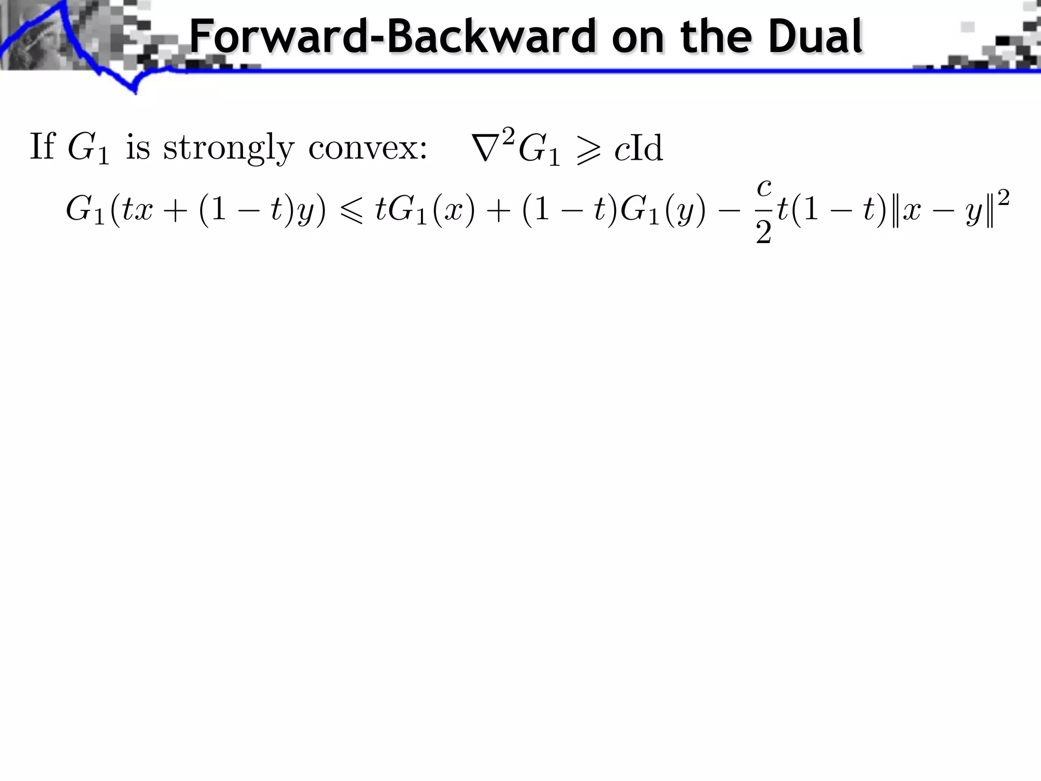
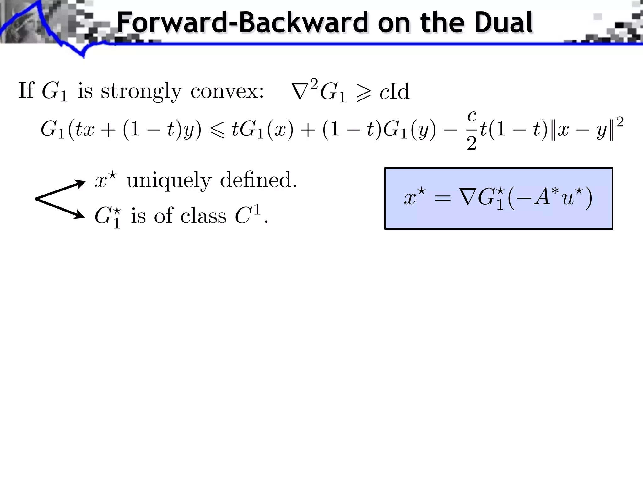
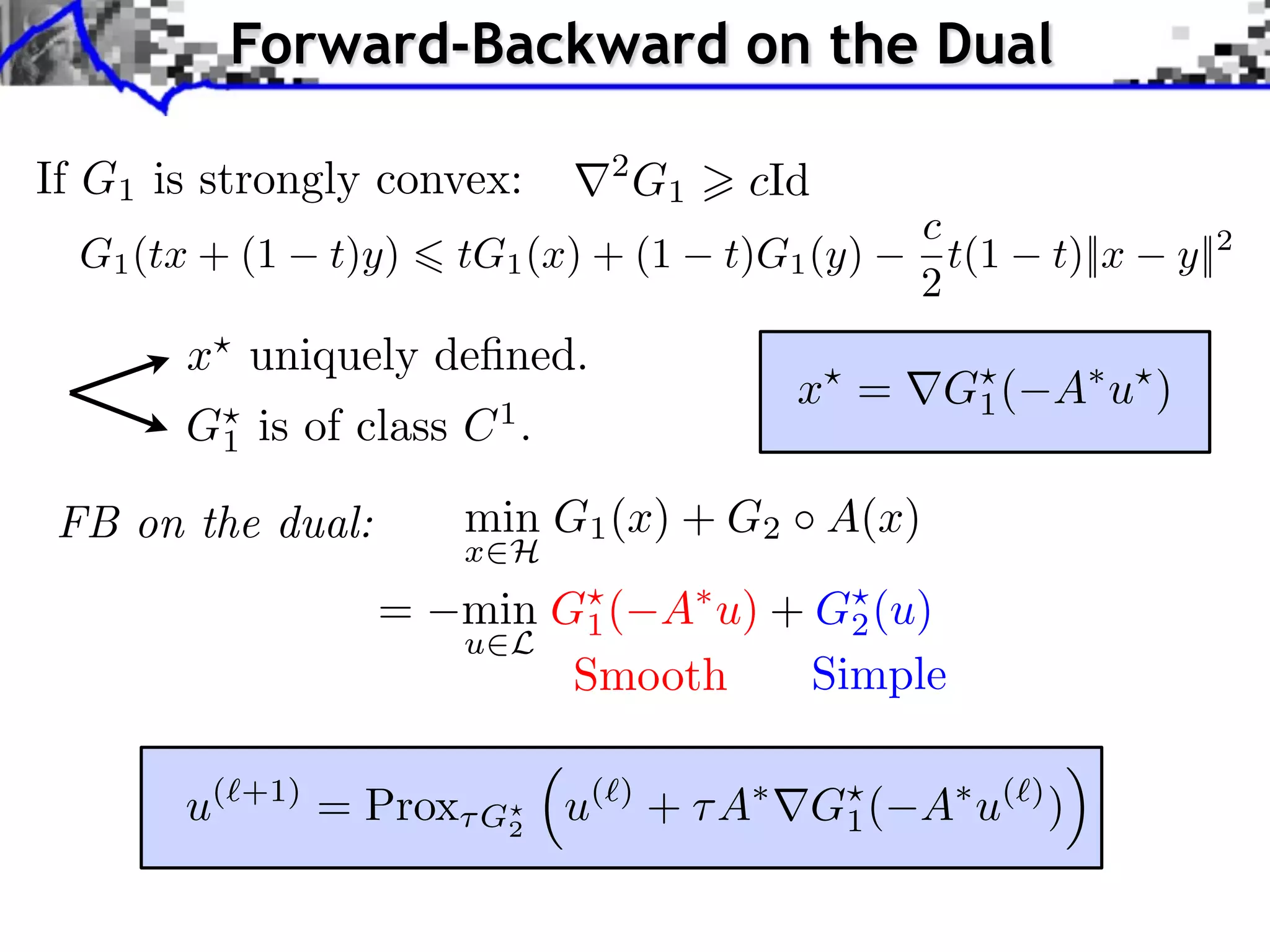
Forward-Backward on the Dual If G1 is strongly convex: r2 G1 > cId c G1 (tx + (1 t)y) 6 tG1 (x) + (1 t)G1 (y) t(1 t)||x y||2 2

Forward-Backward on the Dual If G1 is strongly convex: r2 G1 > cId c G1 (tx + (1 t)y) 6 tG1 (x) + (1 t)G1 (y) t(1 t)||x y||2 2 x? uniquely deﬁned. x? = rG? ( A⇤ u? ) 1 G? is of class C 1 . 1

Forward-Backward on the Dual If G1 is strongly convex: r2 G1 > cId c G1 (tx + (1 t)y) 6 tG1 (x) + (1 t)G1 (y) t(1 t)||x y||2 2 x? uniquely deﬁned. x? = rG? ( A⇤ u? ) 1 G? is of class C 1 . 1 FB on the dual: min G1 (x) + G2 A(x) x2H = min G? ( A⇤ u) + G? (u) 1 2 u2L Smooth Simple ⇣ ⌘ u(`+1) = Prox⌧ G? u(`) + ⌧ A⇤ rG? ( A⇤ u(`) ) 2 1

Example: TV Denoising 1 min ||f y||2 + ||⇥f ||1 min ||y + div(u)||2 f RN 2 ||u|| ||u||1 = ||ui || ||u|| = max ||ui || i i Dual solution u Primal solution f = y + div(u ) [Chambolle 2004]

Example: TV Denoising 1 min ||f y||2 + ||⇥f ||1 min ||y + div(u)||2 f RN 2 ||u|| ||u||1 = ||ui || ||u|| = max ||ui || i i Dual solution u Primal solution f = y + div(u ) FB (aka projected gradient descent): [Chambolle 2004] u( +1) = Proj||·|| u( ) + (y + div(u( ) )) ui v = Proj||·|| (u) vi = max(||ui ||/ , 1) 2 1 Convergence if < = ||div ⇥|| 4

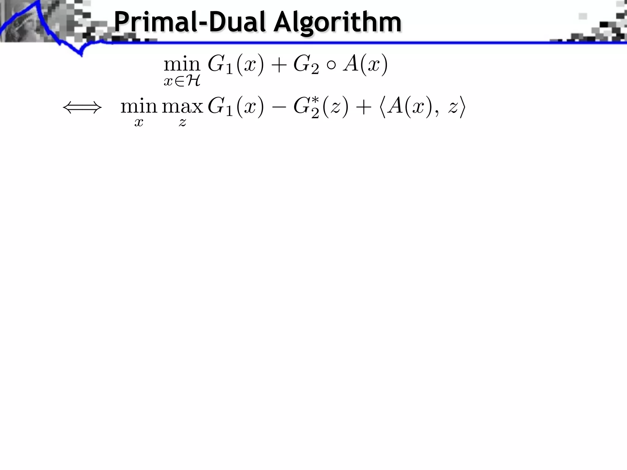
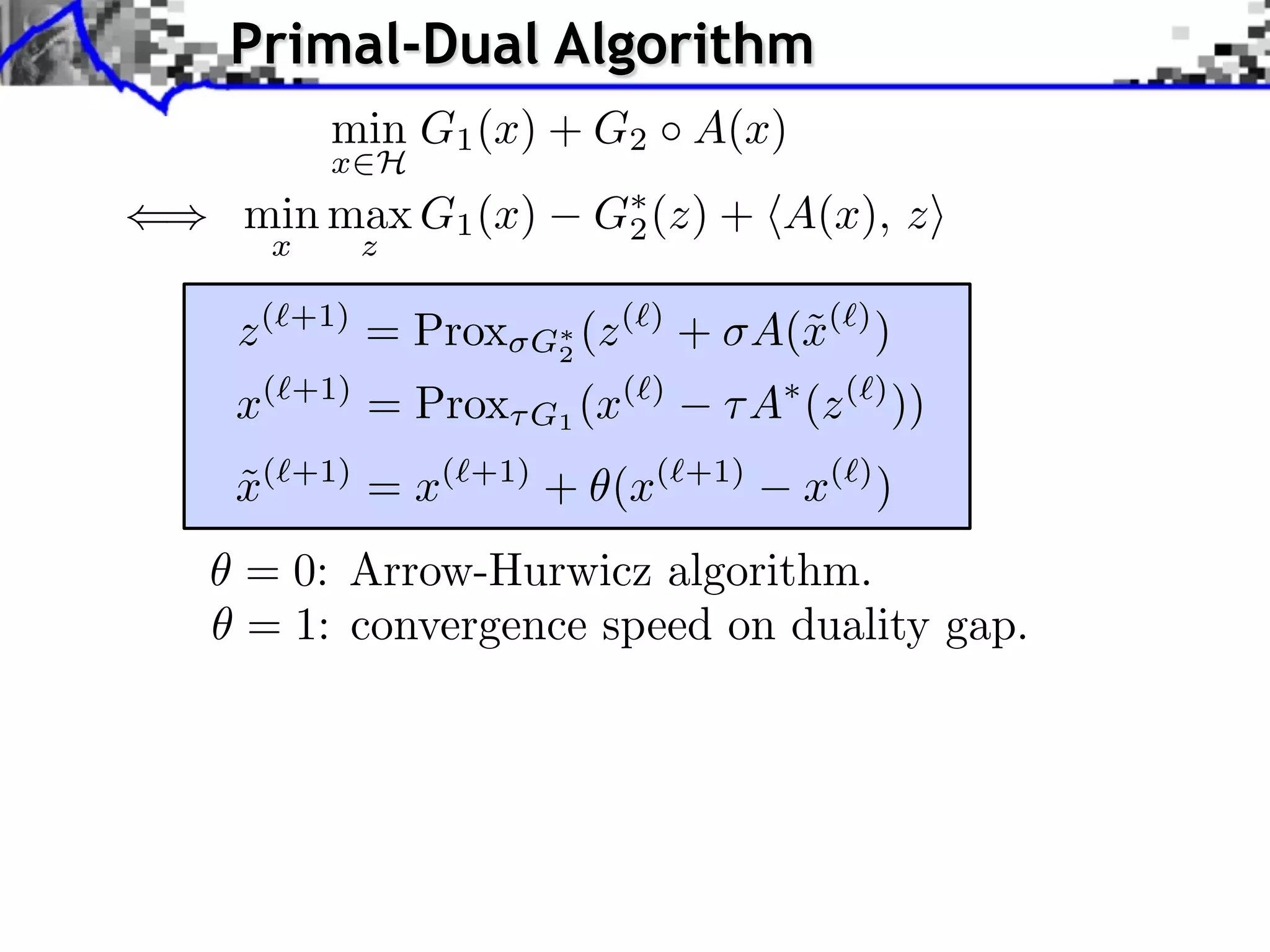
Primal-Dual Algorithm min G1 (x) + G2 A(x) x H () min max G1 (x) G⇤ (z) + hA(x), zi 2 x z

Primal-Dual Algorithm min G1 (x) + G2 A(x) x H () min max G1 (x) G⇤ (z) + hA(x), zi 2 x z z (`+1) = Prox G⇤ 2 (z (`) + A(˜(`) ) x x(⇥+1) = Prox G1 (x(⇥) A (z (⇥) )) ˜ x( +1) = x( +1) + (x( +1) x( ) ) = 0: Arrow-Hurwicz algorithm. = 1: convergence speed on duality gap.

Primal-Dual Algorithm min G1 (x) + G2 A(x) x H () min max G1 (x) G⇤ (z) + hA(x), zi 2 x z z (`+1) = Prox G⇤ 2 (z (`) + A(˜(`) ) x x(⇥+1) = Prox G1 (x(⇥) A (z (⇥) )) ˜ x( +1) = x( +1) + (x( +1) x( ) ) = 0: Arrow-Hurwicz algorithm. = 1: convergence speed on duality gap. Theorem: [Chambolle-Pock 2011] If 0 1 and ⇥⇤ ||A||2 < 1 then x( ) x minimizer of G1 + G2 A.

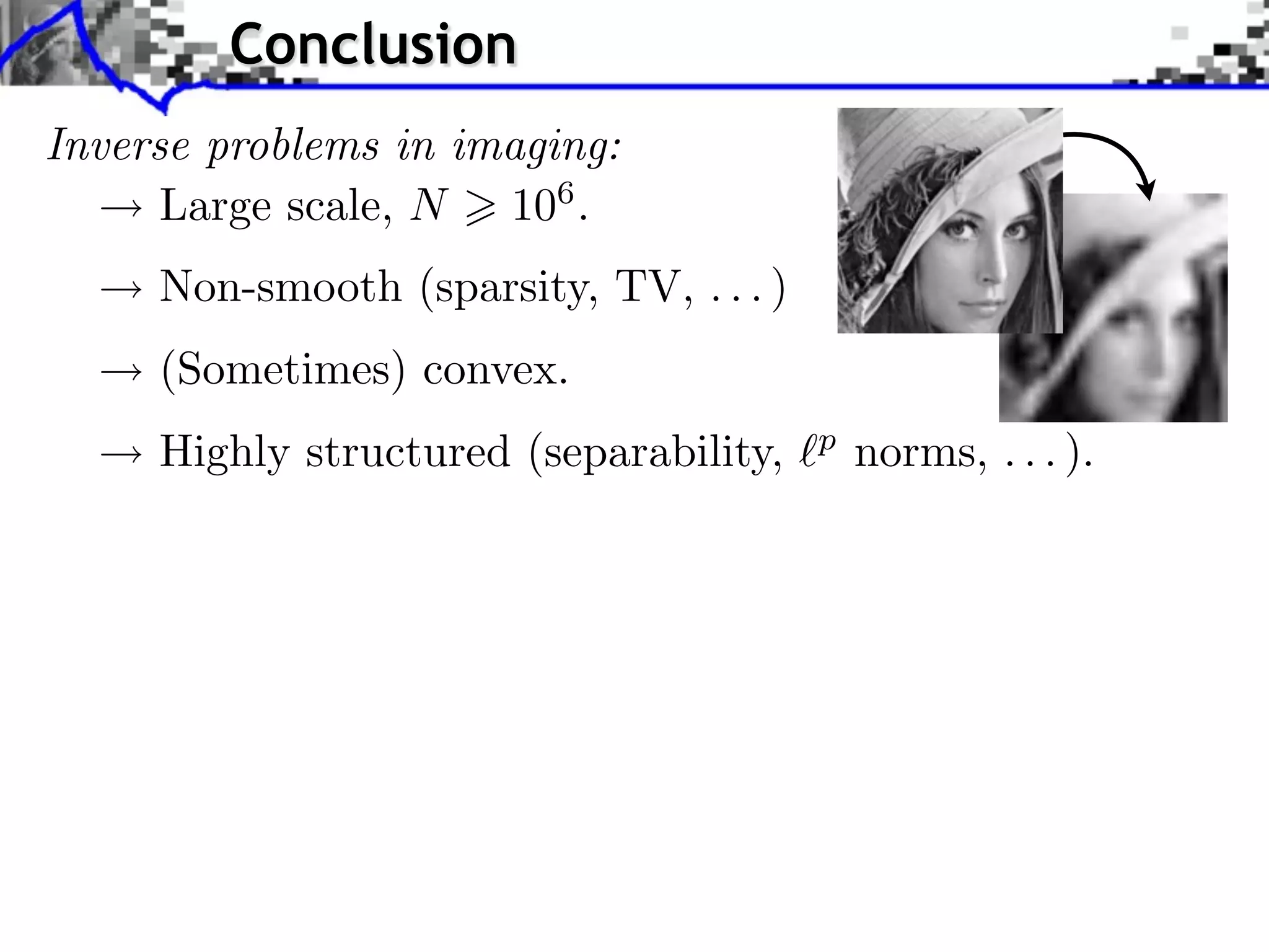
Conclusion Inverse problems in imaging: Large scale, N 106 . Non-smooth (sparsity, TV, . . . ) (Sometimes) convex. Highly structured (separability, p norms, . . . ).

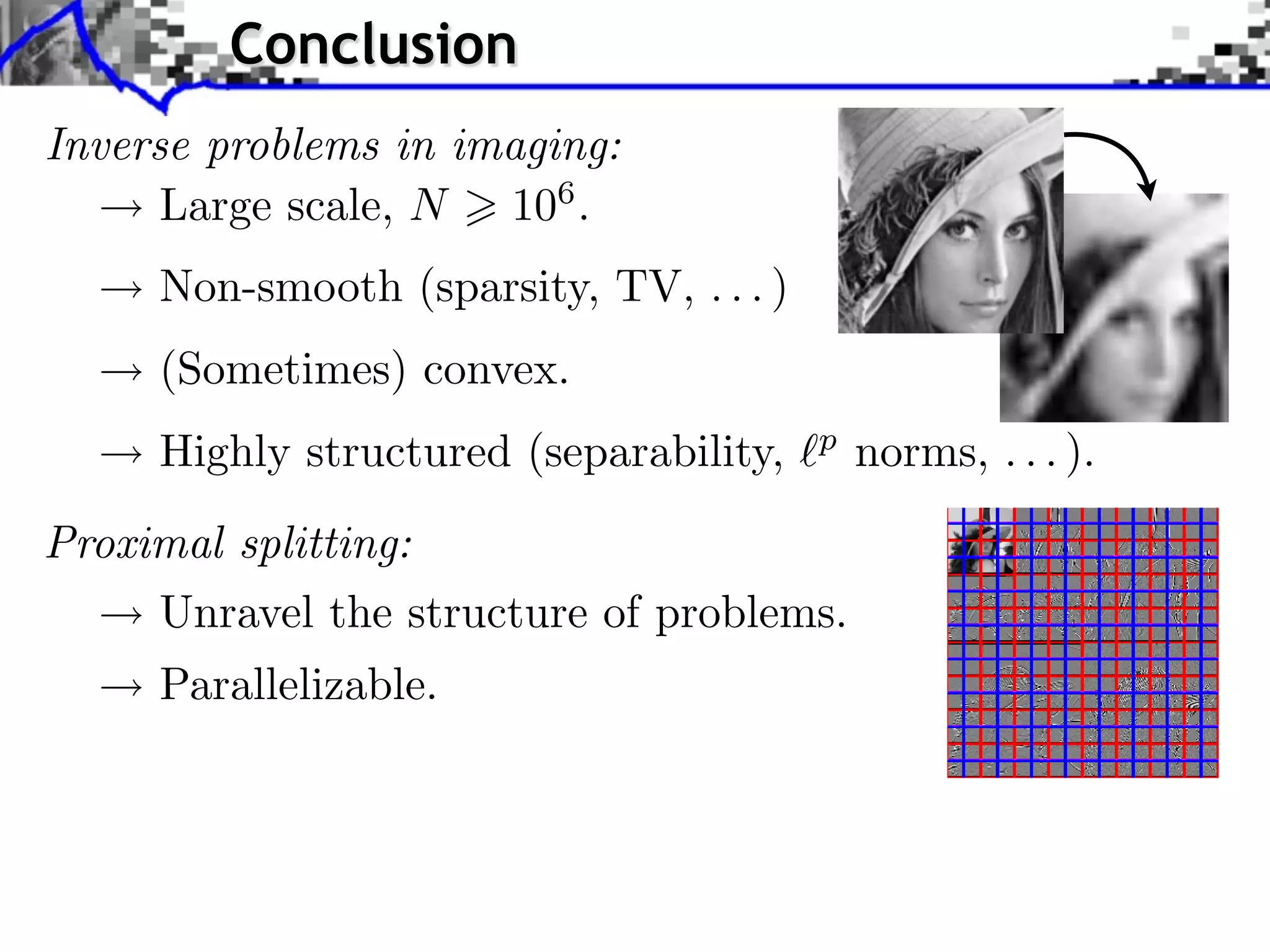
Conclusion Inverse problems in imaging: Large scale, N 106 . Towards More Complex Penalization Non-smooth (sparsity, TV, . . . ) (Sometimes) convex. b B1 i b xi 2 ⇥ x⇥⇥1 = i ⇥xi ⇥ b B 2 i p xi + Highly structured (separability, b norms, . . . ). b B2 i b xi2 Proximal splitting: Unravel the structure of problems. Parallelizable. Decomposition G = k Gk

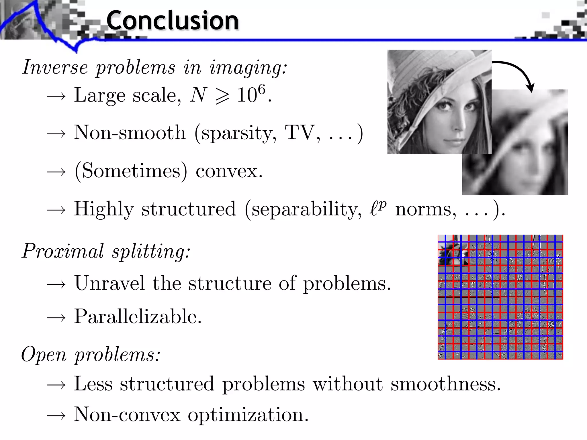
Conclusion Inverse problems in imaging: Large scale, N 106 . Towards More Complex Penalization Non-smooth (sparsity, TV, . . . ) (Sometimes) convex. b B1 i b xi 2 ⇥ x⇥⇥1 = i ⇥xi ⇥ b B 2 i p xi + Highly structured (separability, b norms, . . . ). b B2 i b xi2 Proximal splitting: Unravel the structure of problems. Parallelizable. Open problems: Decomposition G = k Gk Less structured problems without smoothness. Non-convex optimization.

Signal Processing Course : Convex Optimization

More Related Content

What's hot

Viewers also liked

Similar to Signal Processing Course : Convex Optimization

More from Gabriel Peyré

Signal Processing Course : Convex Optimization