Downloaded 21 times
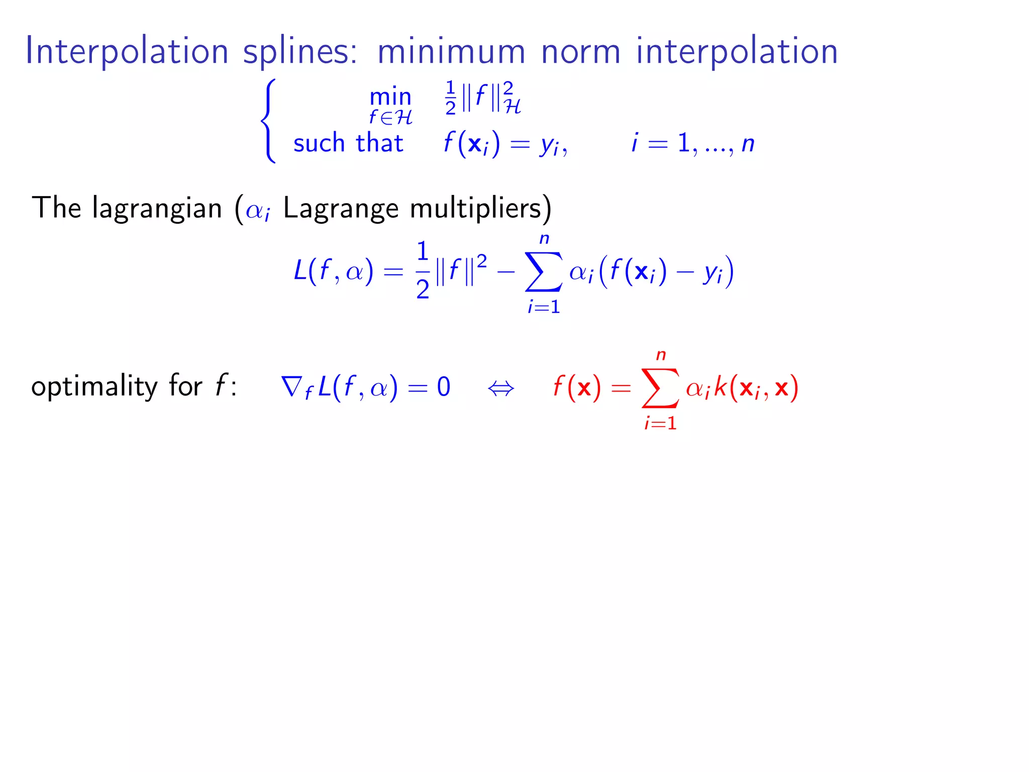
![Regularization path for SVM min f ∈H n i=1 max(1 − yi f (xi ), 0) + λo 2 f 2 H Iα is the set of support vectors s.t. yi f (xi ) = 1; ∂f J(f ) = i∈Iα γi yi K(xi , •) − i∈I1 yi K(xi , •) + λo f (•) with γi ∈ ∂H(1) =] − 1, 0[](https://image.slidesharecdn.com/lecture5kernelsvm-140315083037-phpapp01/75/Lecture5-kernel-svm-25-2048.jpg)
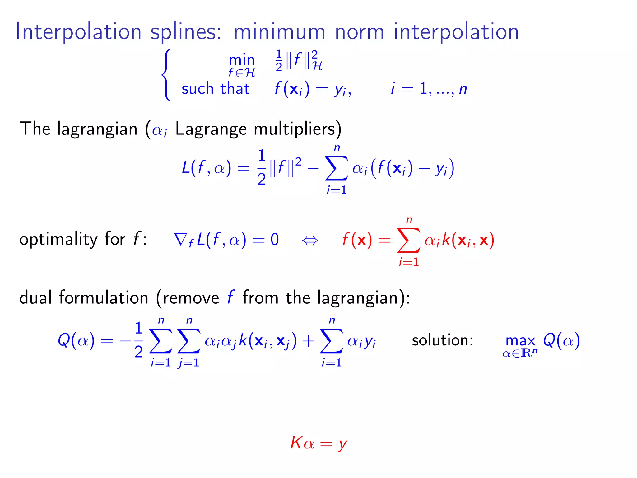
![Regularization path for SVM min f ∈H n i=1 max(1 − yi f (xi ), 0) + λo 2 f 2 H Iα is the set of support vectors s.t. yi f (xi ) = 1; ∂f J(f ) = i∈Iα γi yi K(xi , •) − i∈I1 yi K(xi , •) + λo f (•) with γi ∈ ∂H(1) =] − 1, 0[ Let λn a value close enough to λo to keep the sets I0, Iα and IC unchanged In particular at point xj ∈ Iα (fo(xj ) = fn(xj ) = yj ) : ∂f J(f )(xj ) = 0 i∈Iα γioyi K(xi , xj ) = i∈I1 yi K(xi , xj ) − λo yj i∈Iα γinyi K(xi , xj ) = i∈I1 yi K(xi , xj ) − λn yj G(γn − γo) = (λo − λn)y avec Gij = yi K(xi , xj ) γn = γo + (λo − λn)w w = (G)−1 y](https://image.slidesharecdn.com/lecture5kernelsvm-140315083037-phpapp01/75/Lecture5-kernel-svm-26-2048.jpg)
![Example of regularization path γi ∈] − 1, 0[ yi γi ∈] − 1, −1[ λ = 1 C γi = − 1 C αi ; performing together estimation and data selection](https://image.slidesharecdn.com/lecture5kernelsvm-140315083037-phpapp01/75/Lecture5-kernel-svm-27-2048.jpg)
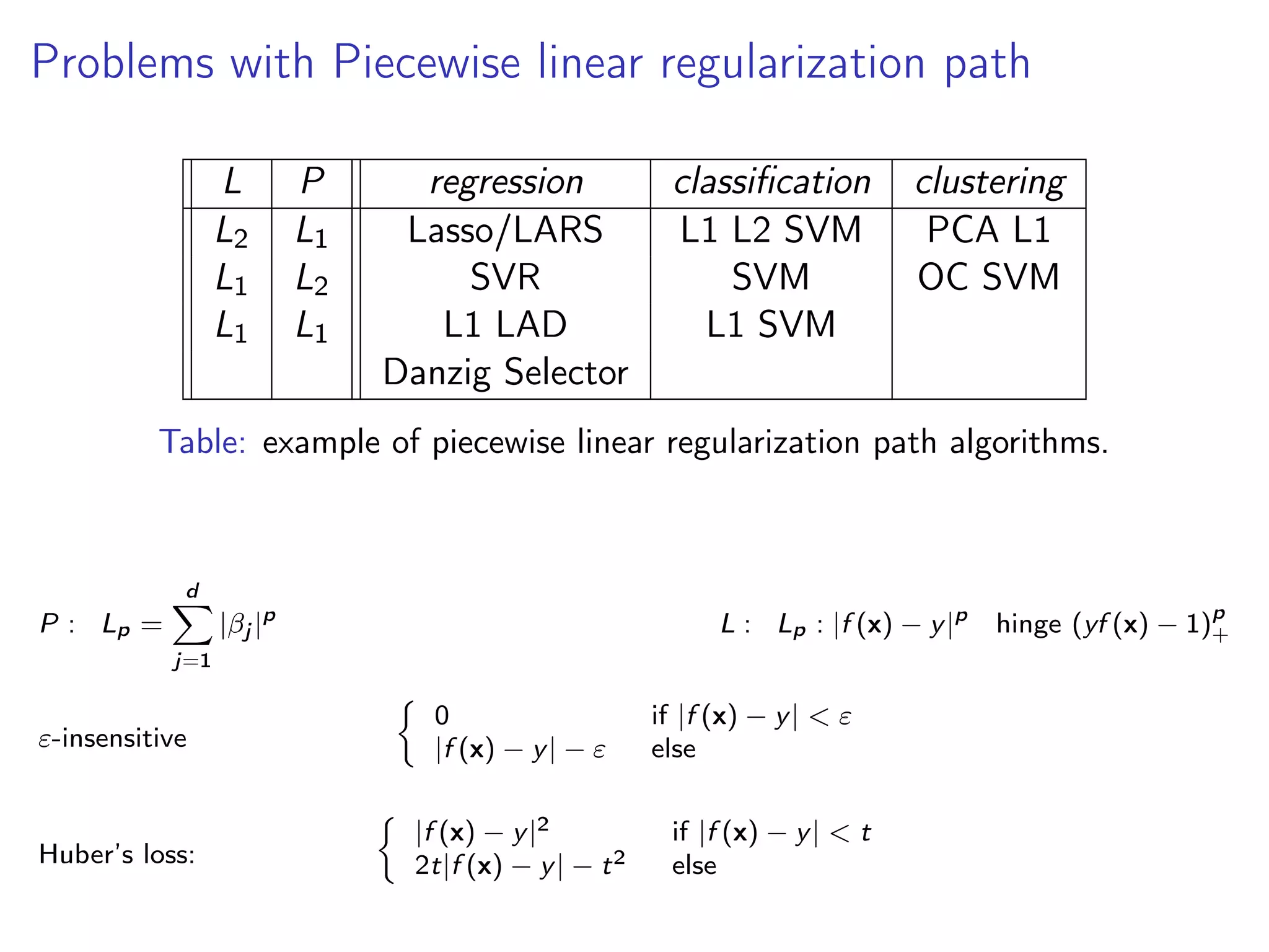
![How to choose and P to get linear regularization path? the path is piecewise linear ⇔ one is piecewise quadratic and the other is piecewise linear the convex case [Rosset & Zhu, 07] min β∈IRd (β) + λP(β) 1 piecewise linearity: lim ε→0 β(λ + ε) − β(λ) ε = constant 2 optimality (β(λ)) + λ P(β(λ)) = 0 (β(λ + ε)) + (λ + ε) P(β(λ + ε)) = 0 3 Taylor expension lim ε→0 β(λ + ε) − β(λ) ε = 2 (β(λ)) + λ 2 P(β(λ)) −1 P(β(λ)) 2 (β(λ)) = constant and 2 P(β(λ)) = 0](https://image.slidesharecdn.com/lecture5kernelsvm-140315083037-phpapp01/75/Lecture5-kernel-svm-28-2048.jpg)
![ν-SVM and other formulations... ν ∈ [0, 1] (ν) min f ,b,ξ,m 1 2 f 2 H + 1 np n i=1 ξp i − νm with yi f (xi ) + b ≥ m − ξi , i = 1, n, and m ≥ 0, ξi ≥ 0, i = 1, n, for p = 1 the dual formulation is: max α∈IRn −1 2 α Gα with α y = 0 et 0 ≤ αi ≤ 1 n i = 1, n and ν ≤ α 1I C = 1 m](https://image.slidesharecdn.com/lecture5kernelsvm-140315083037-phpapp01/75/Lecture5-kernel-svm-31-2048.jpg)

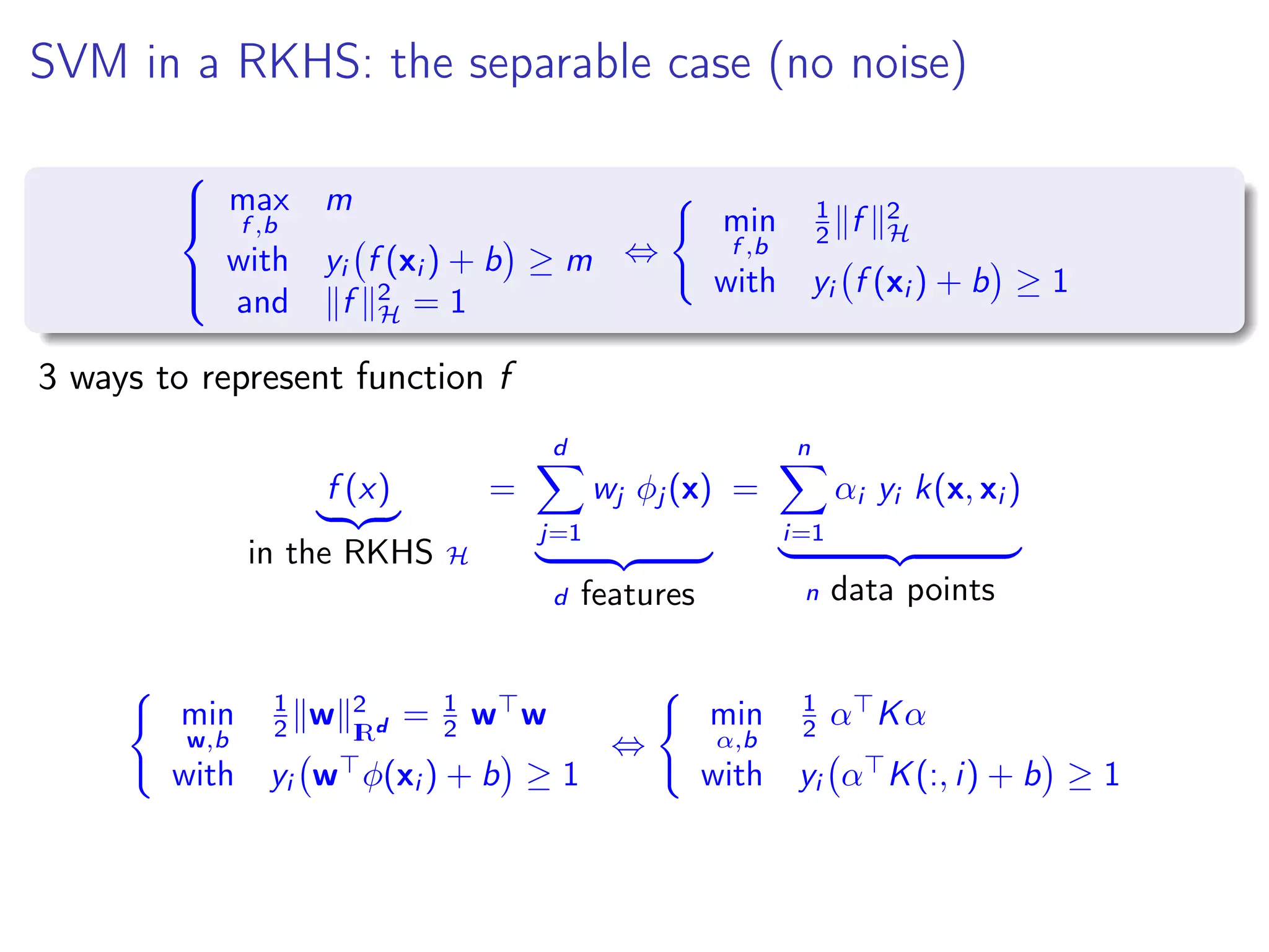
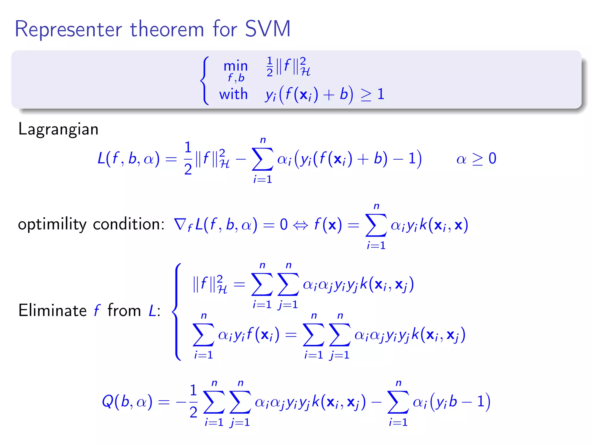
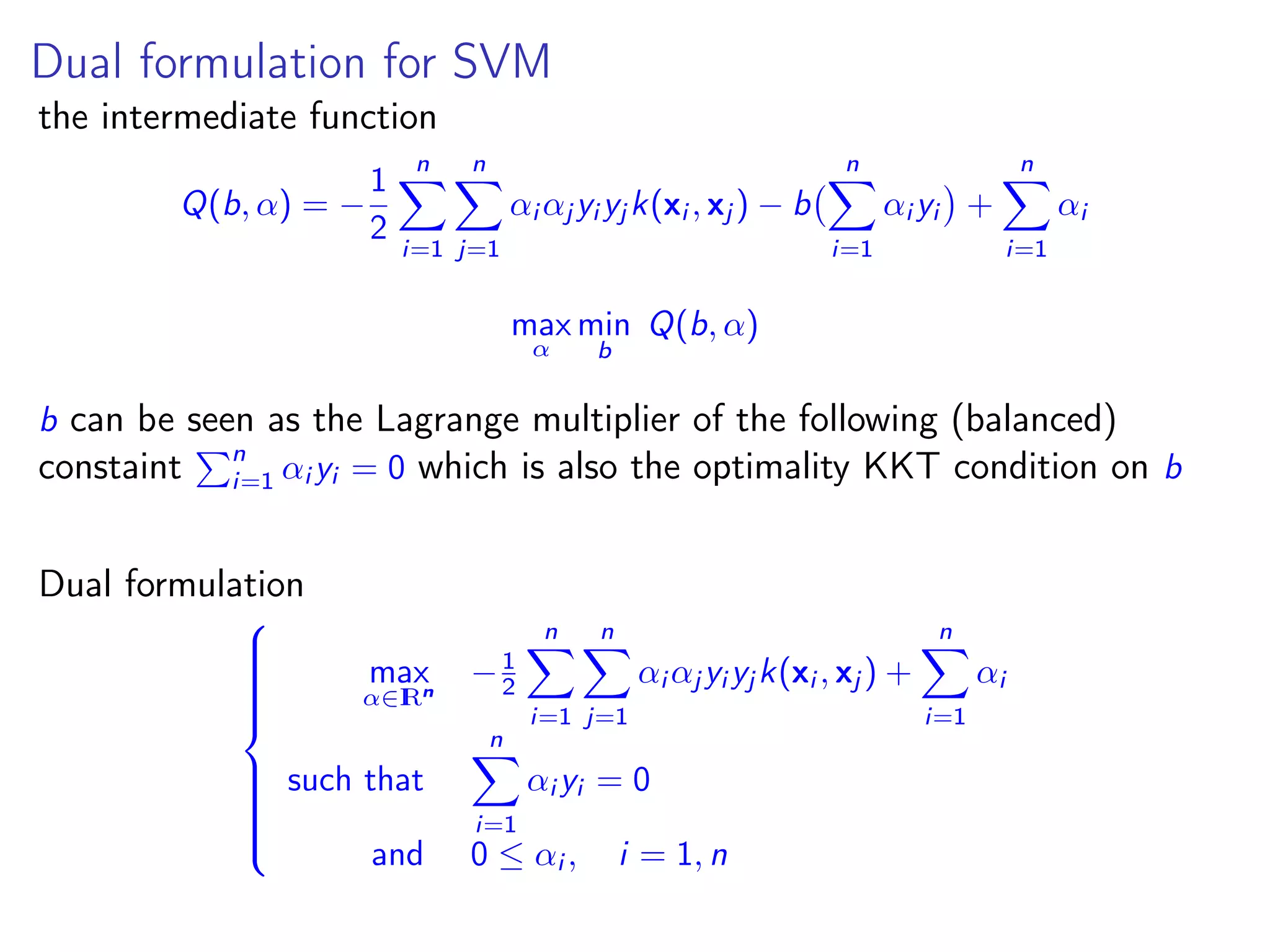
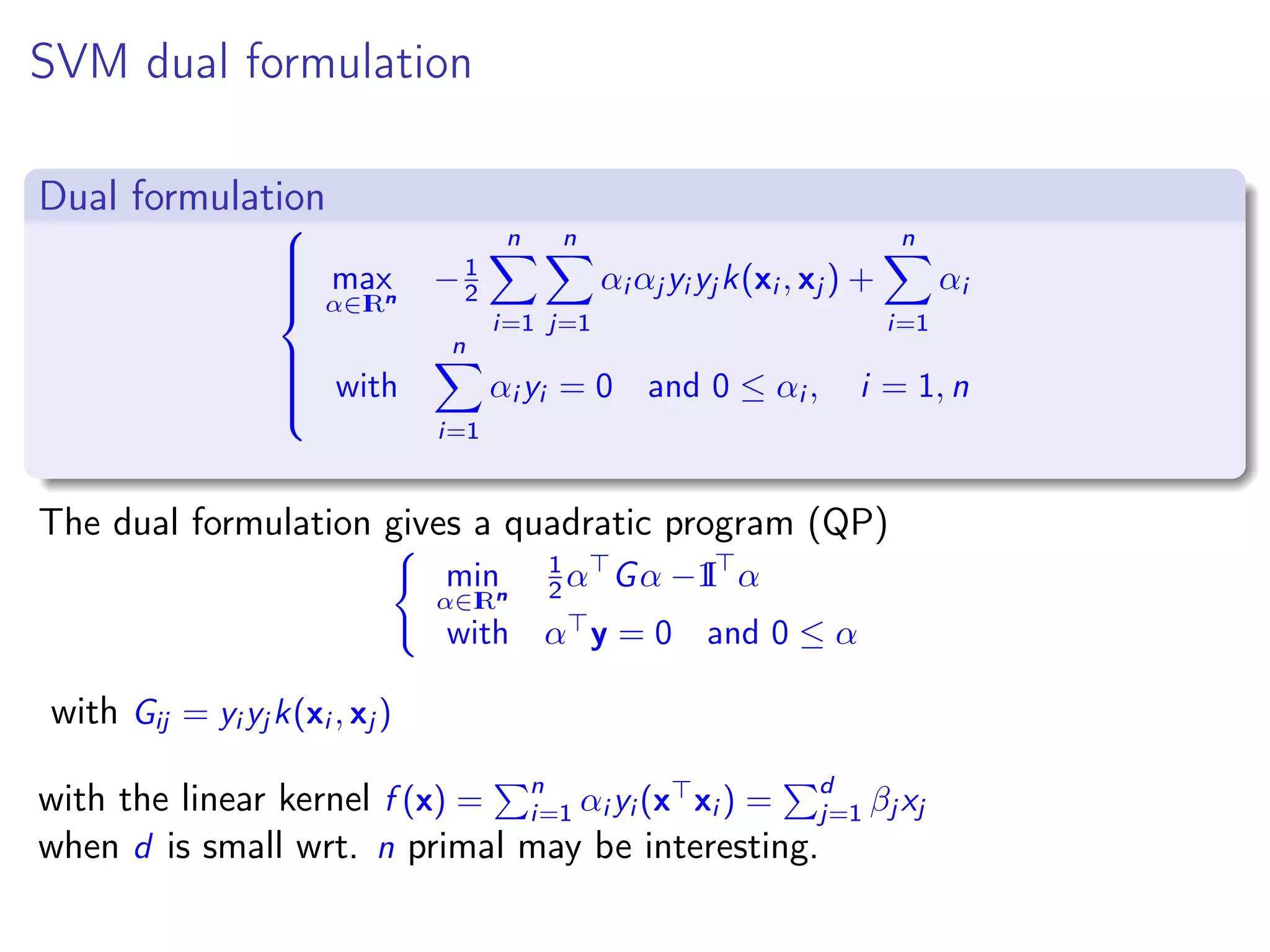
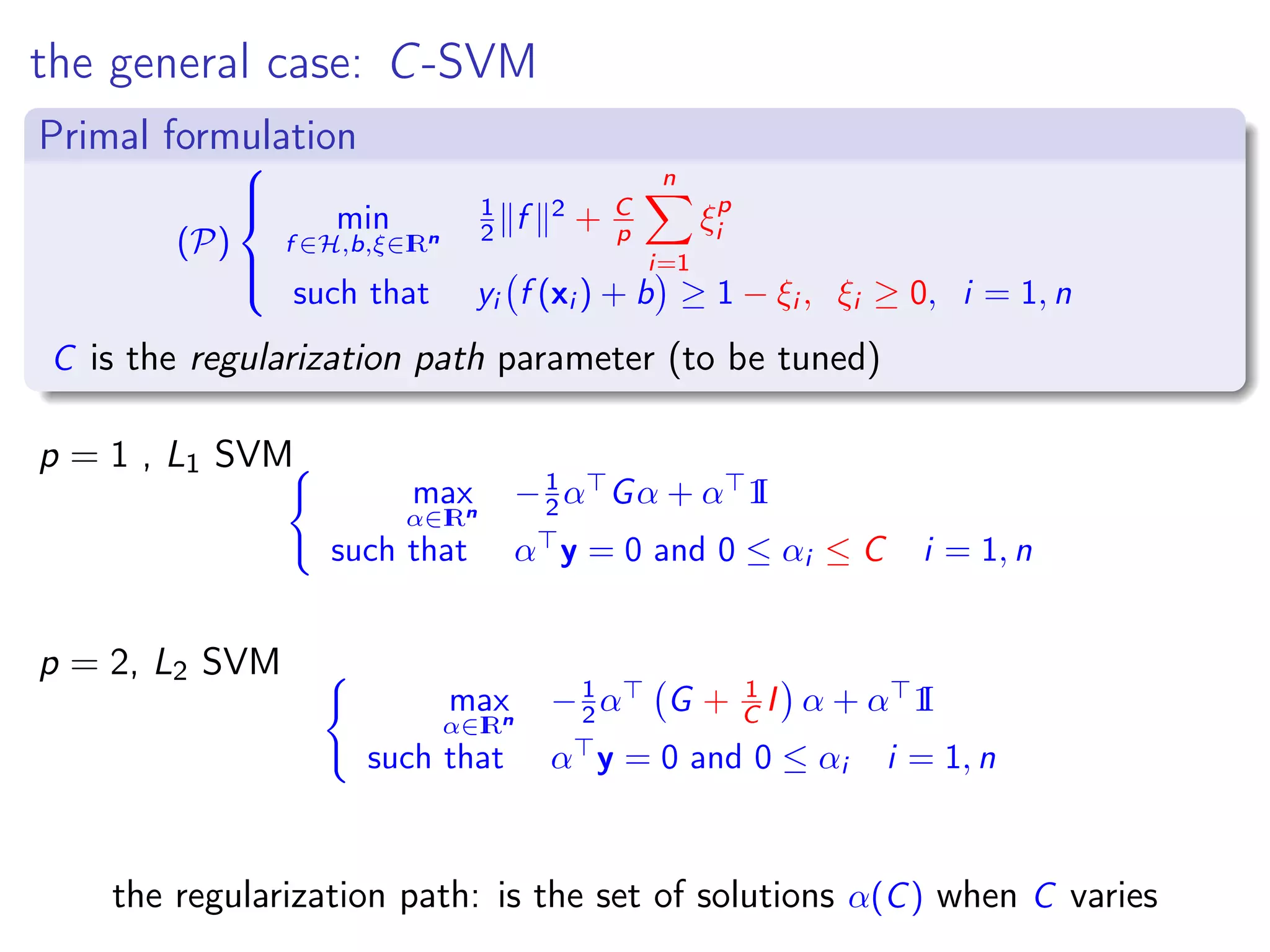
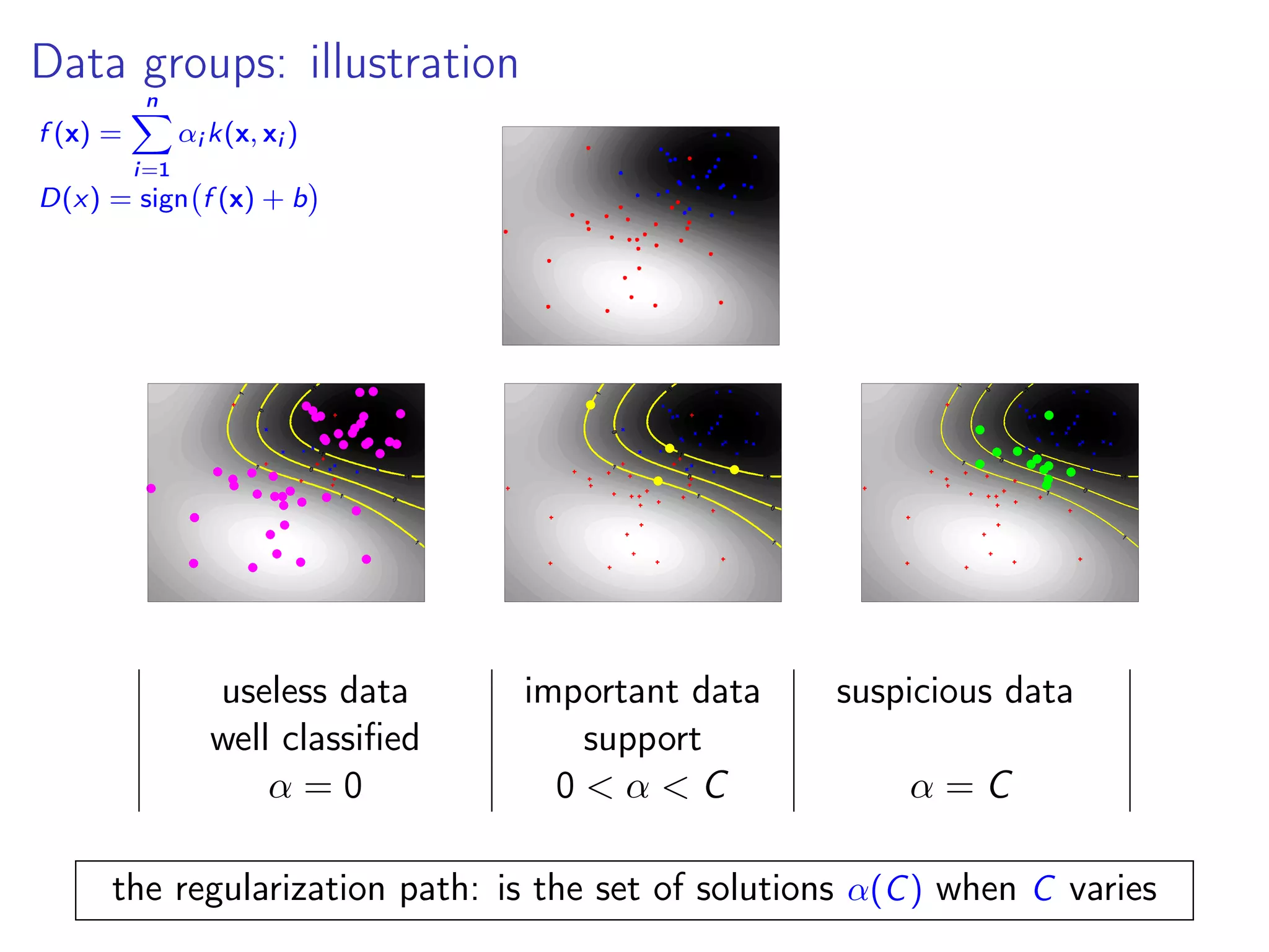
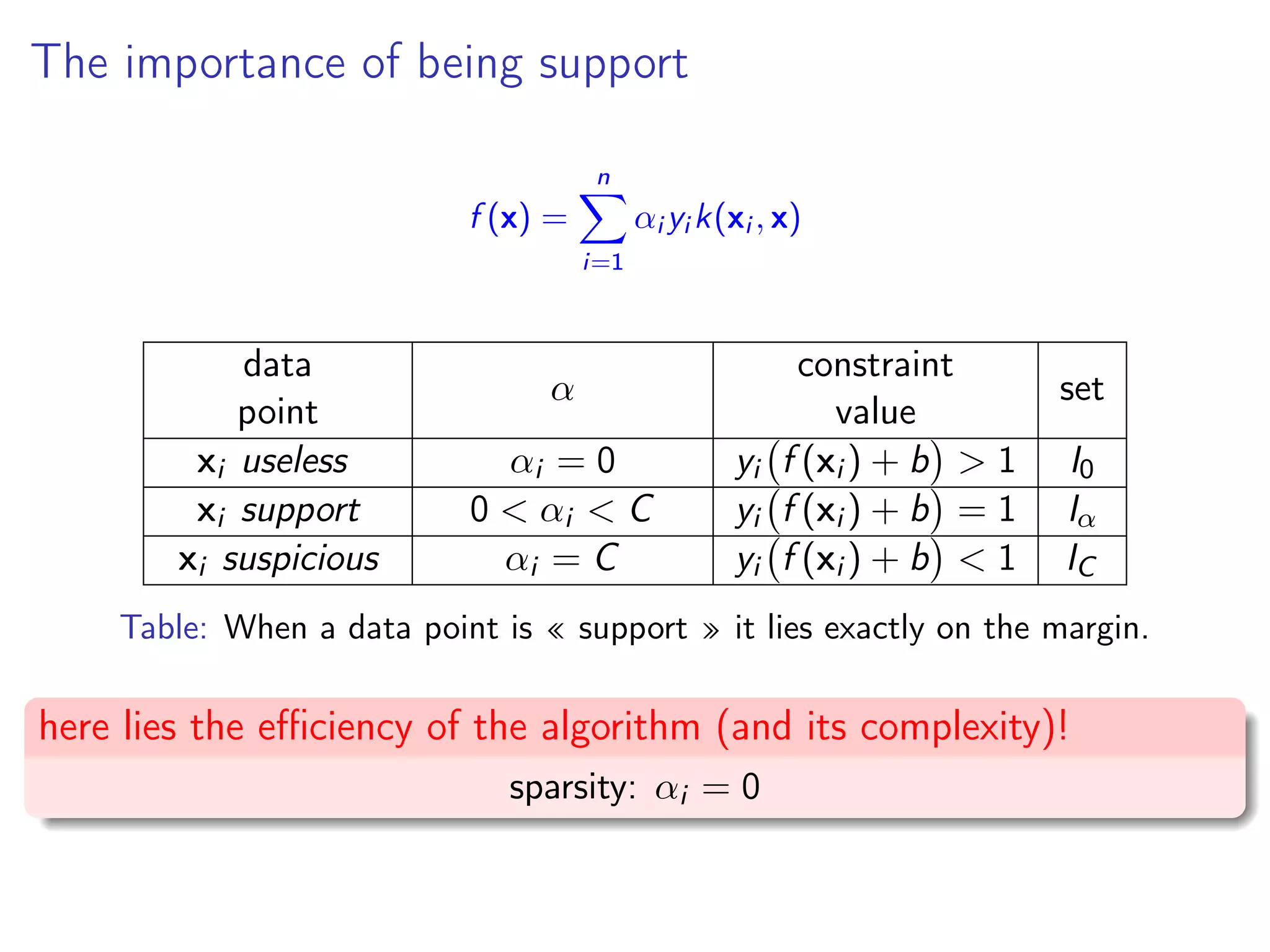
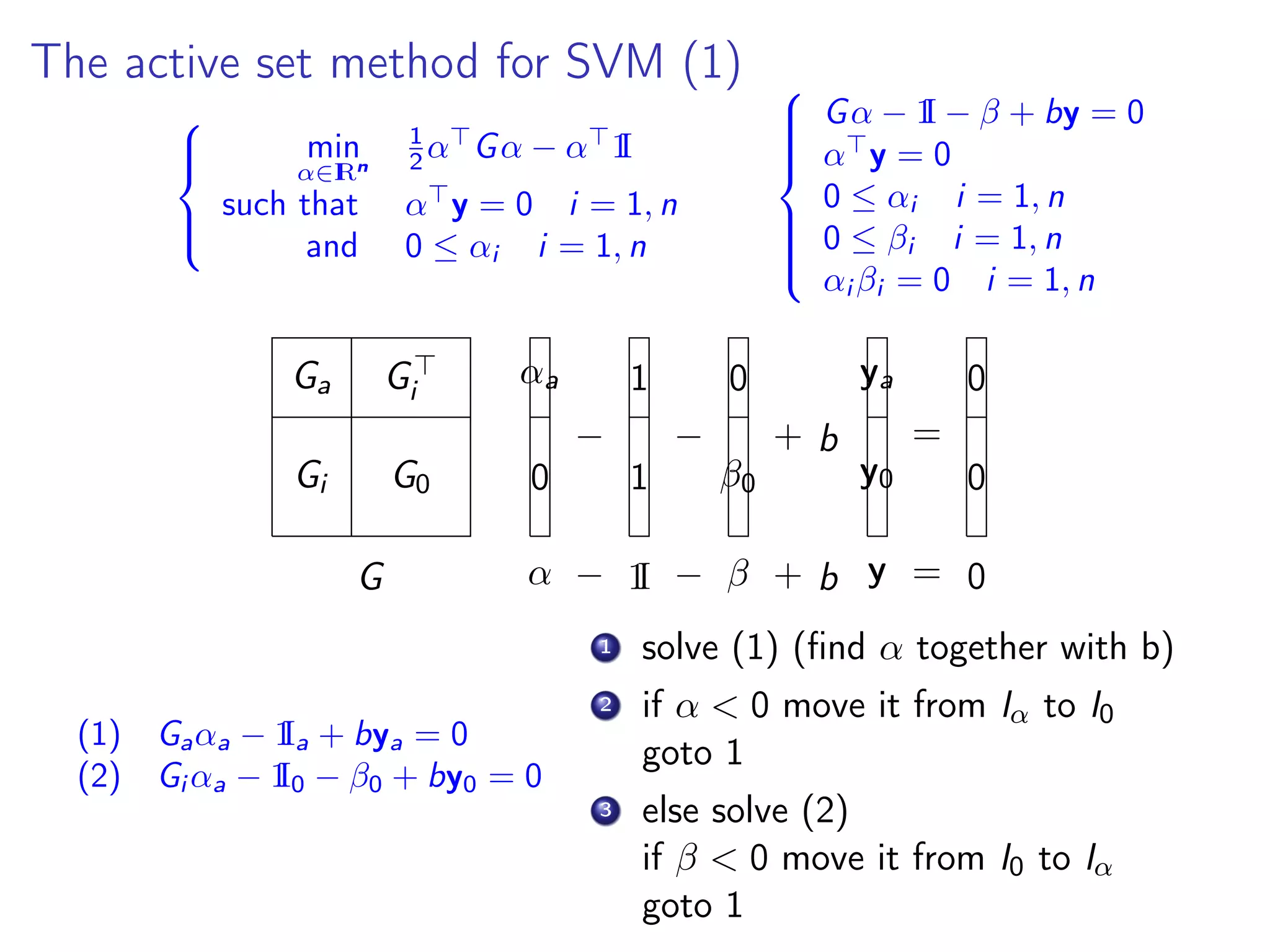
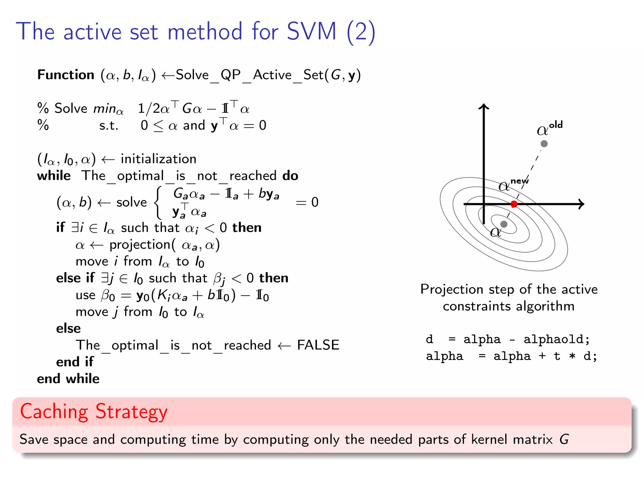
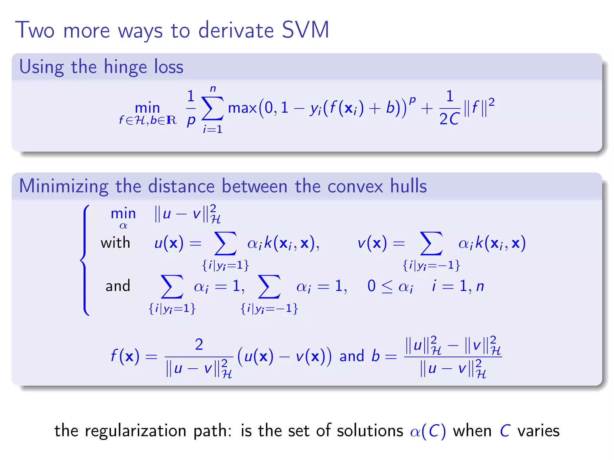
This document provides an overview of support vector machines (SVMs) as kernel machines. It discusses how SVMs can be formulated as optimization problems in reproducing kernel Hilbert spaces using kernels. Specifically, it covers: 1) How the SVM primal optimization problem can be solved using Lagrange multipliers and the representer theorem to obtain the dual quadratic program. 2) How the regularization parameter C in the C-SVM formulation allows data points to lie on or outside the margin. 3) The active set method for solving the SVM quadratic program, which iteratively optimizes over the sets of active and inactive constraints.