Download to read offline

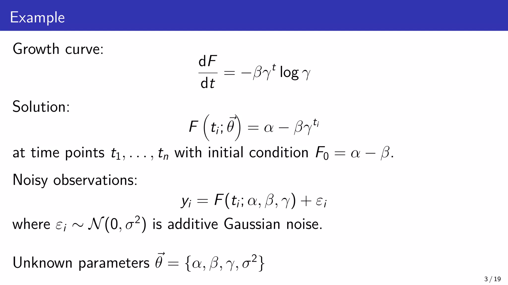


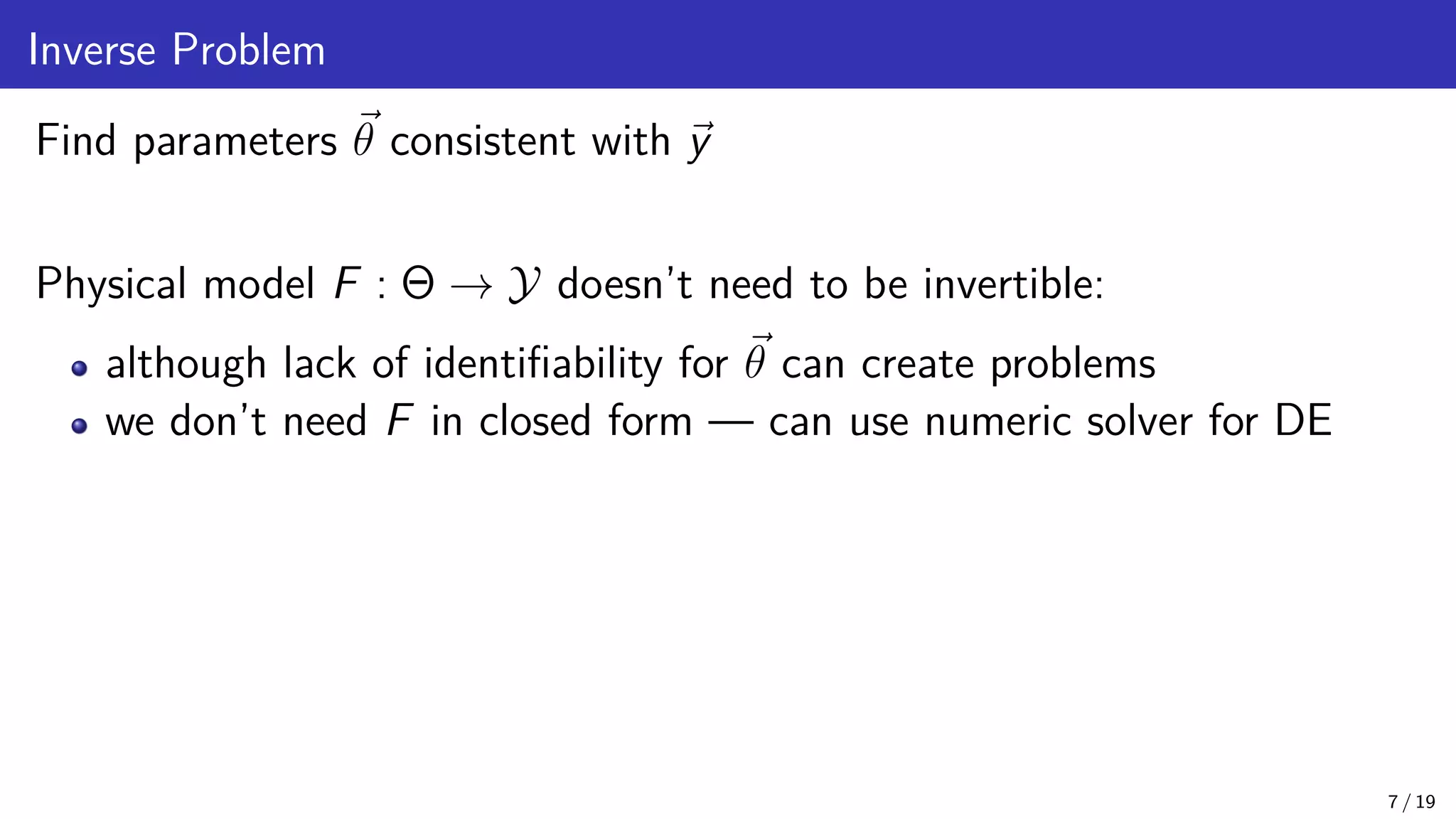
![Inverse Problem Find parameters ~ θ consistent with ~ y Physical model F : Θ → Y doesn’t need to be invertible: although lack of identifiability for ~ θ can create problems we don’t need F in closed form — can use numeric solver for DE Likelihood L(~ y | ~ θ) is based on E[Yi | ~ θ] = F ti; ~ θ as well as distribution of random noise (not necessarily Gaussian) 7 / 19](https://image.slidesharecdn.com/moorestide20211014-211014093220/75/Bayesian-Inference-and-Uncertainty-Quantification-for-Inverse-Problems-13-2048.jpg)

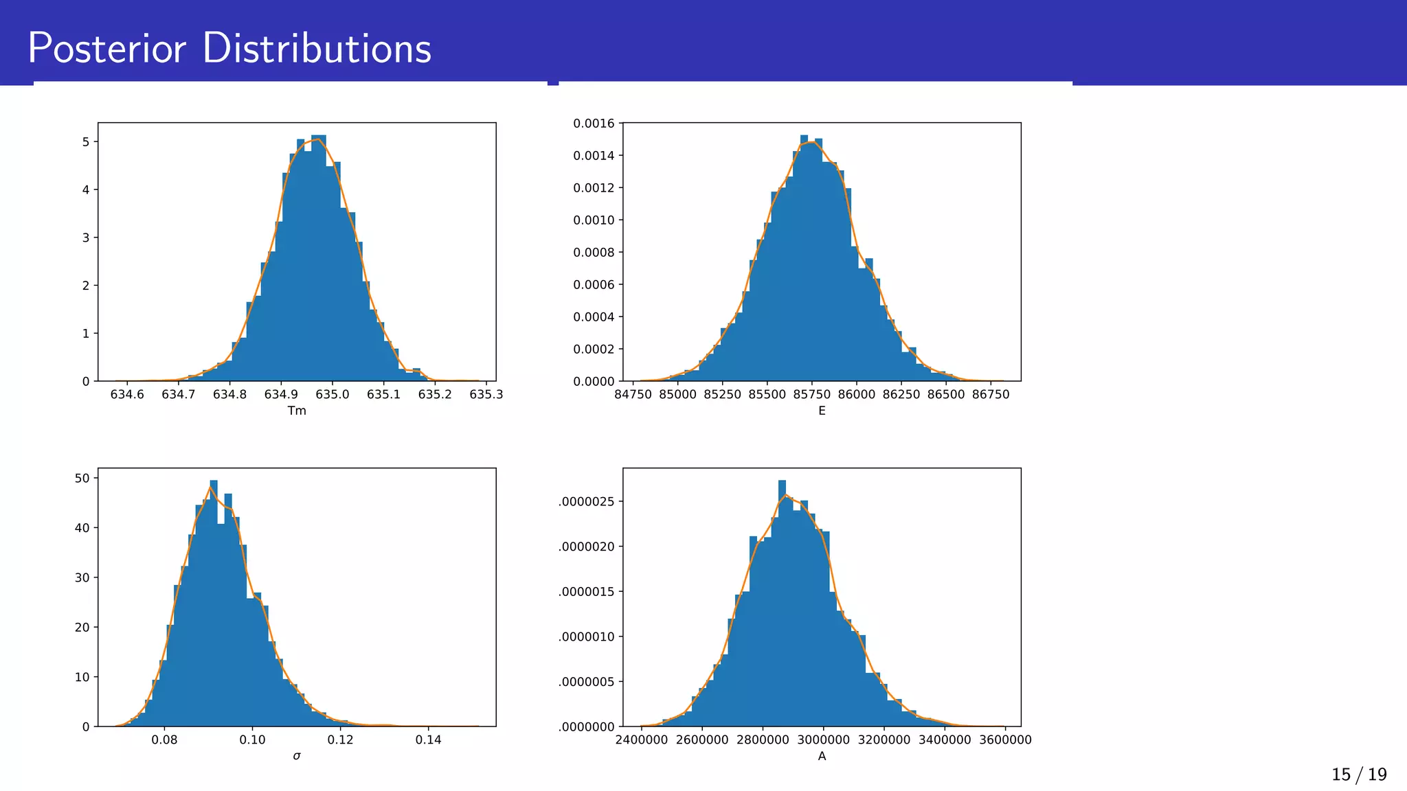
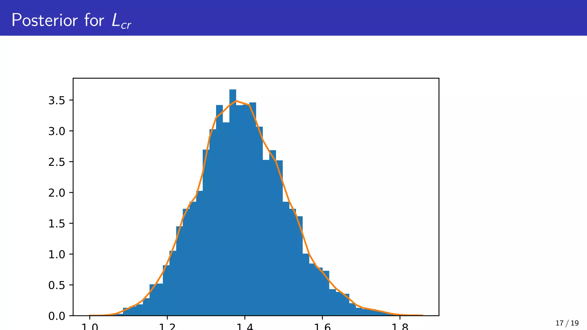
![Posterior for Functions of ~ θ A function of a random variable is also a random variable. Now that we have random samples from our posterior π(A, E, Tm, σ2 | ~ y), we can use our model to obtain predictions for any measurable function of the parameters, g(A, E, Tm). For example, the critical length of a stockpile: Lcr = g(A, E, Tm) = K v u u texp n E RT2 m o A RT2 m E E[g(A, E, Tm) | ~ y] = Z 1000 0 Z ∞ 0 Z ∞ 0 g(A, E, Tm) dπ(A, E, Tm | ~ y) ≈ J X j=1 g(Aj, Ej, Tj) where K is a constant and {Aj, Ej, Tj}J j=1 are the MCMC samples (after discarding burn-in). 16 / 19](https://image.slidesharecdn.com/moorestide20211014-211014093220/75/Bayesian-Inference-and-Uncertainty-Quantification-for-Inverse-Problems-25-2048.jpg)


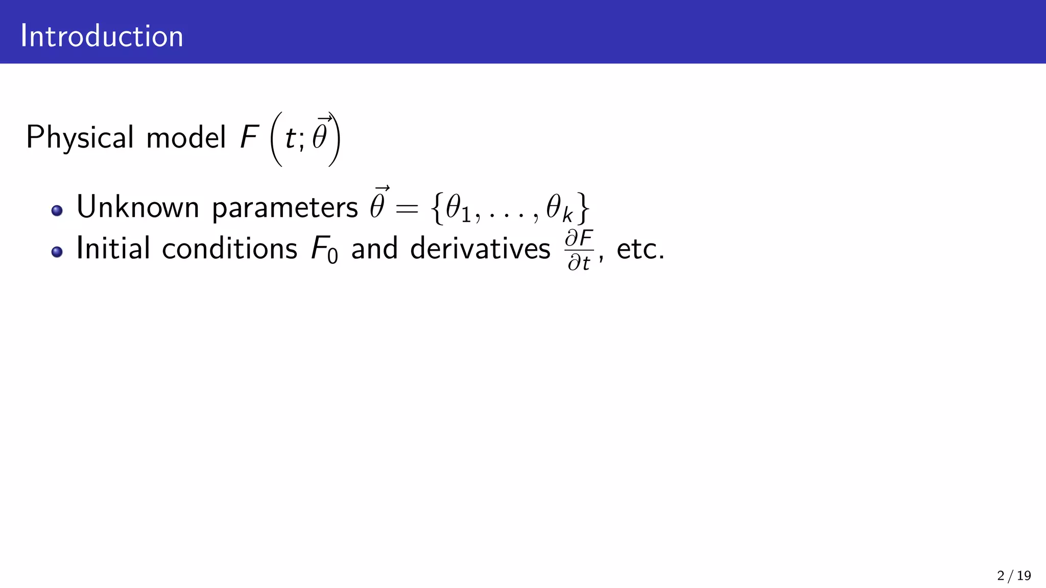
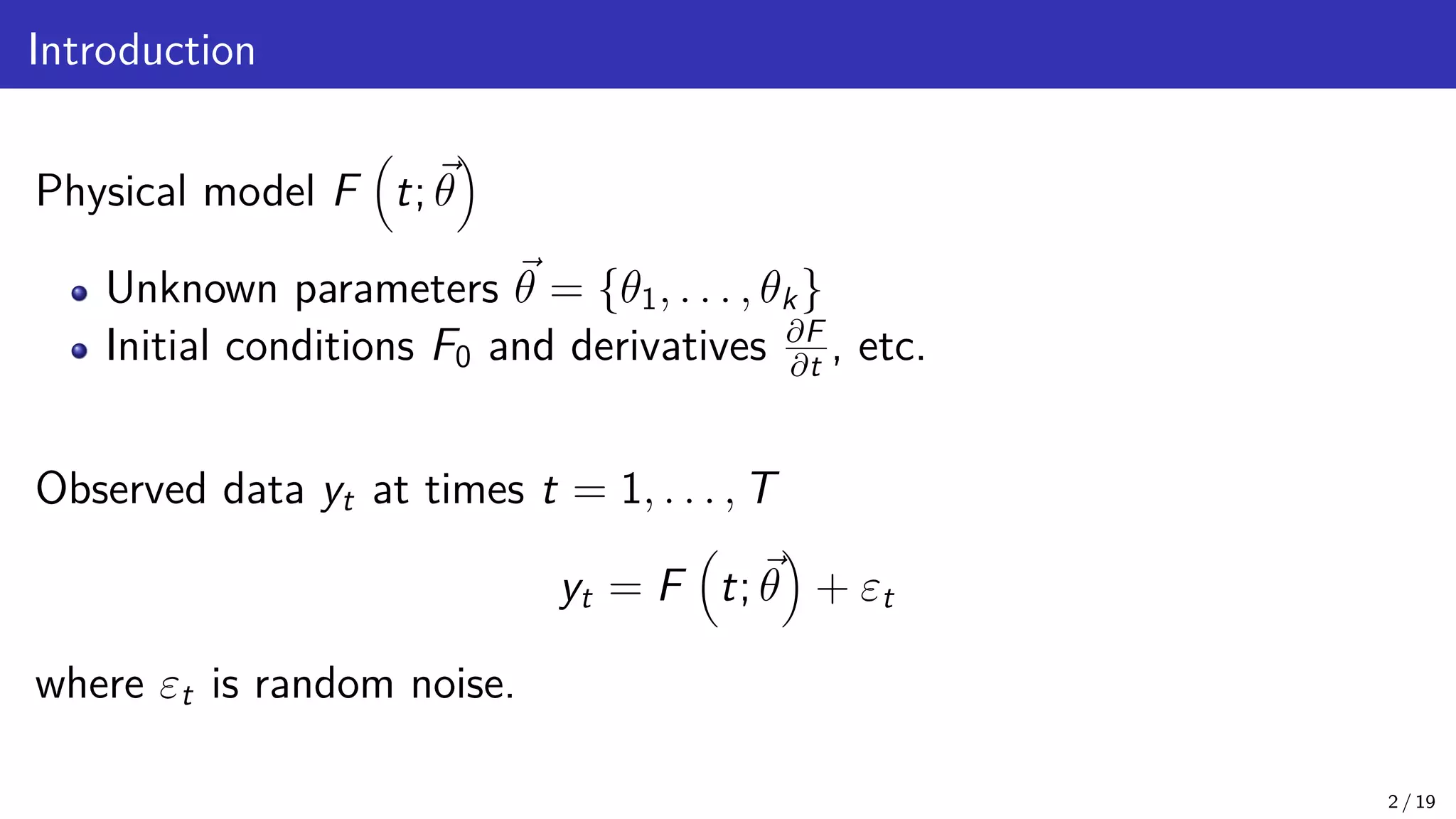
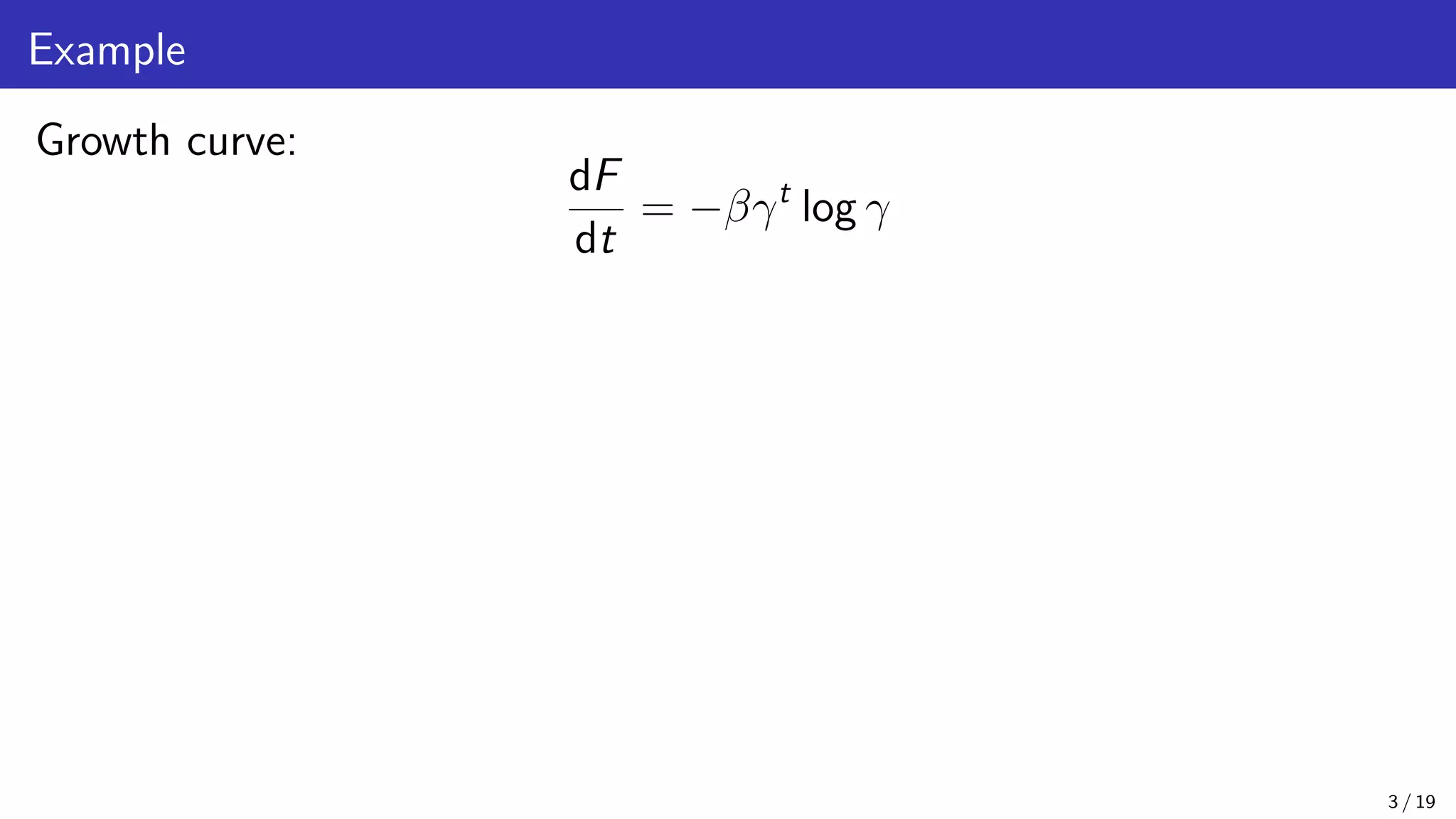
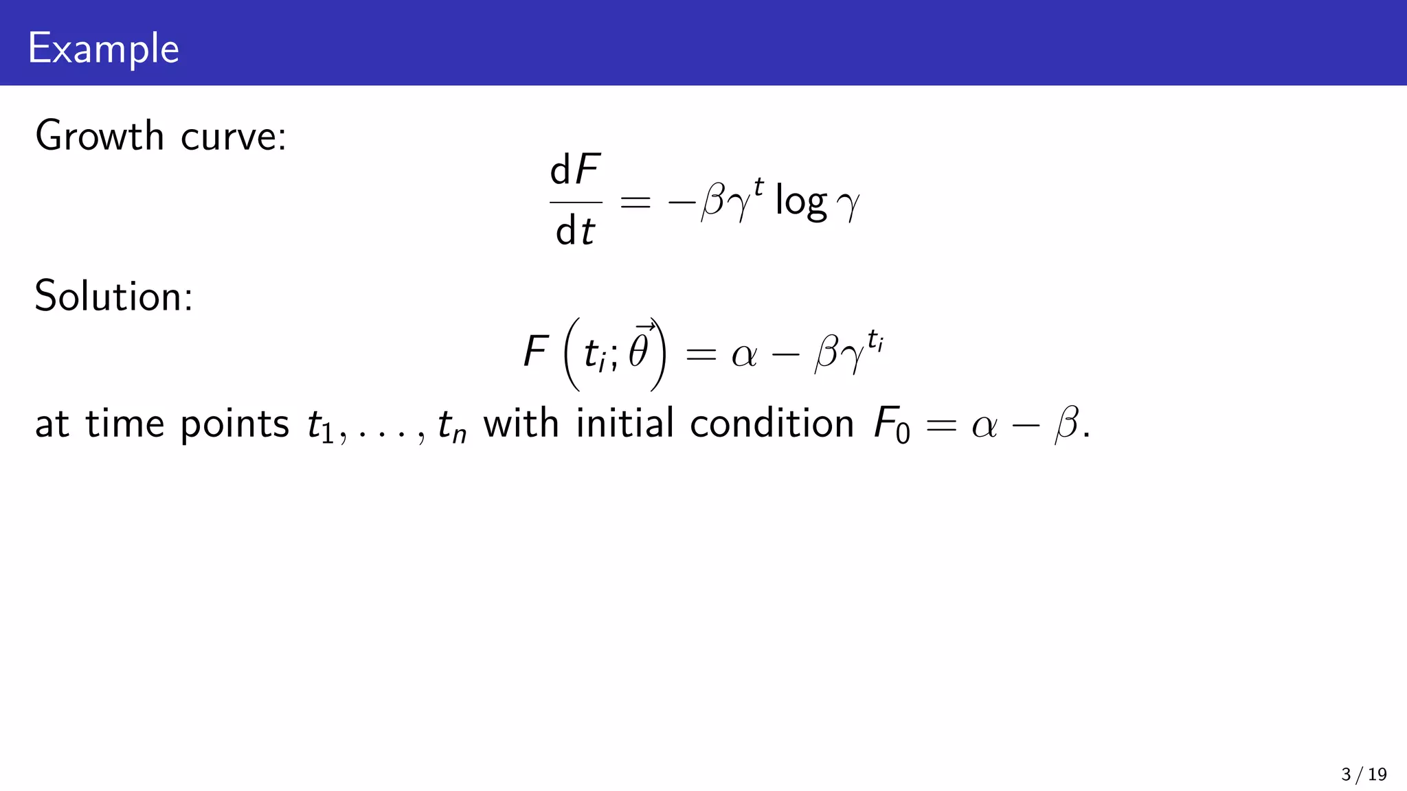
The document discusses Bayesian inference and uncertainty quantification applied to inverse problems, detailing the process of finding unknown parameters using observed data, models, and prior distributions. It highlights the use of Markov Chain Monte Carlo methods and offers examples, particularly in contexts like population growth curves and thermogravimetric analysis. Additionally, advanced methods for improving computational efficiency and addressing model complexities are mentioned.