Inference for stochastic differential equations via approximate Bayesian computation

Inference for SDE models via Approximate Bayesian Computation Umberto Picchini Centre for Mathematical Sciences, Lund University, Sweden www.maths.lth.se/matstat/staff/umberto/ Nordstat, Umeå 13 June 2012 1 / 21 Inference for SDE models via Approximate Bayesian Computation

Motivations The study of complex systems requires multidimensional models. These are often deﬁned on different scales, with several unknown parameters to be estimated from data. Systems are often “partially observed” → latent variables; Measurement error is typically a non-negligible source of variability; Dynamical systems might evolve randomly → stochastic differential equations (SDEs); Systems biology applications are examples of problems involving the “complications” above. 2 / 21 Inference for SDE models via Approximate Bayesian Computation

Goal of this talk Inference for stochastic systems modelled by SDEs observed at discrete time points is complicated and has generated a large amount of literature in the past 20 years. the exploitation of MCMC methodology produced in the ’90s has broken several barriers and allowed exploration of complex inferential problems like never before; the availability of more affordable computational resources has made the application of intense computational algorithms more viable. however MCMC methodology for Bayesian inference (e.g. Metropolis-Hastings) does not scale well for large systems, i.e. the resulting chain might have poor mixing, resulting in unacceptably long computational times. Goal is to consider Approximate Bayesian Computation to alleviate inferential problems in relatively “large”/complex SDE models. 3 / 21 Inference for SDE models via Approximate Bayesian Computation

We are interested in estimating parameters from observation {yi}i=1,...,n generated from the following state-space model: dXt = µ(Xt, t, ψ)dt + σ(Xt, t, ψ)dWt Yti = f(Xti , εti ), εti ∼ N(0, σ2 εId), i = 1, .., n Xti may be multidimensional ∈ Rd and partially observed; the εi are to be interpreted as i.i.d measurement error terms independent of Wt. And w.l.g we assume: Yi = Xti + εti , i = 1, ..., n Our goal is to estimate θ = (ψ, σε) conditionally on observations y = {y0, y1, ..., yn} using Bayesian methodology. 4 / 21 Inference for SDE models via Approximate Bayesian Computation

Bayesian inference about θ is based on the (marginal) posterior density π(θ | y) ∝ l(θ; y)π(θ) We assume that the likelihood function l(θ; y) may be unavailable for mathematical reasons (not available in closed from) or for computational reasons (too expensive to calculate). In our case data: y = (y0, y1, ..., yn) obtained at times {t0, ..., tn} i.e. yi ≡ yti and x = (x0, x1, ..., xn) is the SDE solution at time-points {t0, ..., tn}. l(θ; y) = π(y | θ) = π(y | x; θ)π(x | θ)dx → “data augmentation” from θ to (x, θ) use MCMC to deal with the multiple integration problem. Because of increased dimension (from θ to (θ, x)) convergence properties of MCMC algorithms are too poor for the algorithm to be considered. [Marin, Pudlo, Robert and Ryder 2011] 5 / 21 Inference for SDE models via Approximate Bayesian Computation

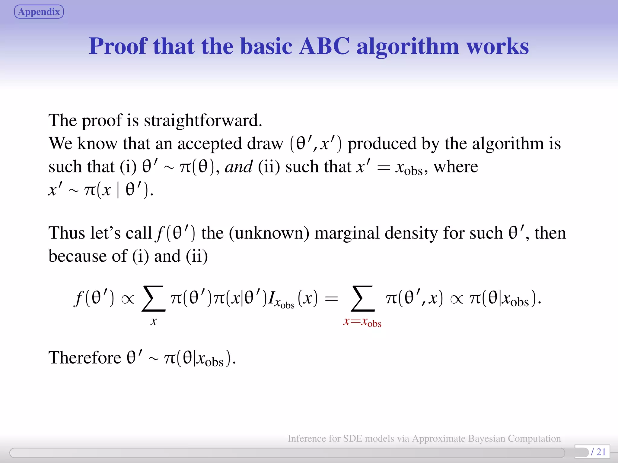
Approximate Bayesian Computation (ABC, ﬁrst proposed in Tavaré et al., 1997) bypass the computation of the likelihood function. Basic ABC idea (for sake of simplicity: no measurement error here): for an observation xobs ∼ π(x | θ), under the prior π(θ), keep jointly simulating θ ∼ π(θ), x ∼ π(x | θ ) until the simulated variable x is equal to the observed one, x = xobs. Then a θ satisfying such condition is such that θ ∼ π(θ | xobs). [Tavaré et al., 1997]. proof The equality x = xobs can’t usually be expected for large discrete systems, and holds with zero probability for vectors x = (xt0 , ..., xtn ) resulting from a diffusion process. Choose instead an accuracy threshold δ; substitute “accept if x = xobs” with “accept if ρ(S(x ), S(xobs)) < δ” for some measure ρ(·) and statistic S(·). 6 / 21 Inference for SDE models via Approximate Bayesian Computation

Acceptance probability in Metropolis-Hastings Suppose at a given iteration of Metropolis-Hastings that the (augmented)-state is (θ#, x#) and wonder whether to move (or not) to a new state (θ , x ). The move is generated via a proposal distribution “q((θ#, x#) → (x , θ ))”. e.g. “q((θ#, x#) → (x , θ ))” = u(θ |θ#)v(x | θ ); move “(θ# , x# ) → (θ , x )” accepted with probability α(θ#,x#)→(x ,θ ) = min 1, π(θ )π(x |θ )π(y|x , θ )q((θ , x ) → (θ#, x#)) π(θ#)π(x#|θ#)π(y|x#, θ#)q((θ#, x#) → (θ , x )) = min 1, π(θ )π(x |θ )π(y|x , θ )u(θ#|θ )v(x# | θ#) π(θ#)π(x#|θ#)π(y|x#, θ#)u(θ |θ#)v(x | θ ) now choose v(x | θ) ≡ π(x | θ) = min 1, π(θ )π(x |θ )π(y|x , θ )u(θ#|θ ) π(x# | θ#) π(θ#)π(x#|θ#)π(y|x#, θ#)u(θ |θ#) π(x | θ ) This is likelihood–free! And we only need to know how to generate x (not a problem...) 7 / 21 Inference for SDE models via Approximate Bayesian Computation

As from the previous slide, for dynamical problems we only need to know how to generate a proposal x = (x0, ..., xn) ⇒ for SDEs: use Euler-Maruyama, Milstein, Stochastic RK discretizations etc. The simplest approximation scheme to the SDE solution (Euler–Maruyama): given an SDE: dXt = µ(Xt, ψ)dt + σ(Xt, ψ)dWt approximate with Xt = Xt−h + µ(Xt−h, ψ)h + σ(Xt−h, ψ)(Wt − Wt−h) [approximation converge to the exact solution for h → 0] and we can interpolate on such approximation at discrete times {t0, t1, ..., tn} to obtain the corresponding “latent states” x = {x0, x1, ..., xn}. 8 / 21 Inference for SDE models via Approximate Bayesian Computation

We now plug the previous ideas in a MCMC ABC algorithm [Sisson-Fan, 2011] 1. Choose or simulate θstart ∼ π(θ) and xstart ∼ usually unknown! π(x|θstart) . Fix δ 0 and r = 0. Put θr = θstart and (supposedly known!) statistics S(xr) ≡ S(xstart). At (r + 1)th MCMC iteration: 2. generate θ ∼ u(θ |θr) from its proposal distribution; 3. generate x ∼ π(x |θ ) and calculate S(x ); 4. with probability min 1, π(θ )πδ(y|x ,θ ))u(θr|θ ) π(θr)πδ(y|xr,θr)u(θ |θr) set (θr+1, S(xr+1)) = (θ , S(x )) otherwise set (θr+1, S(xr+1)) = (θr, S(xr)); 5. increment r to r + 1 and go to step 2. with e.g. πδ(y | x, θ) = 1 δK |S(x)−S(y)| δ [Bloom 2010]. 9 / 21 Inference for SDE models via Approximate Bayesian Computation

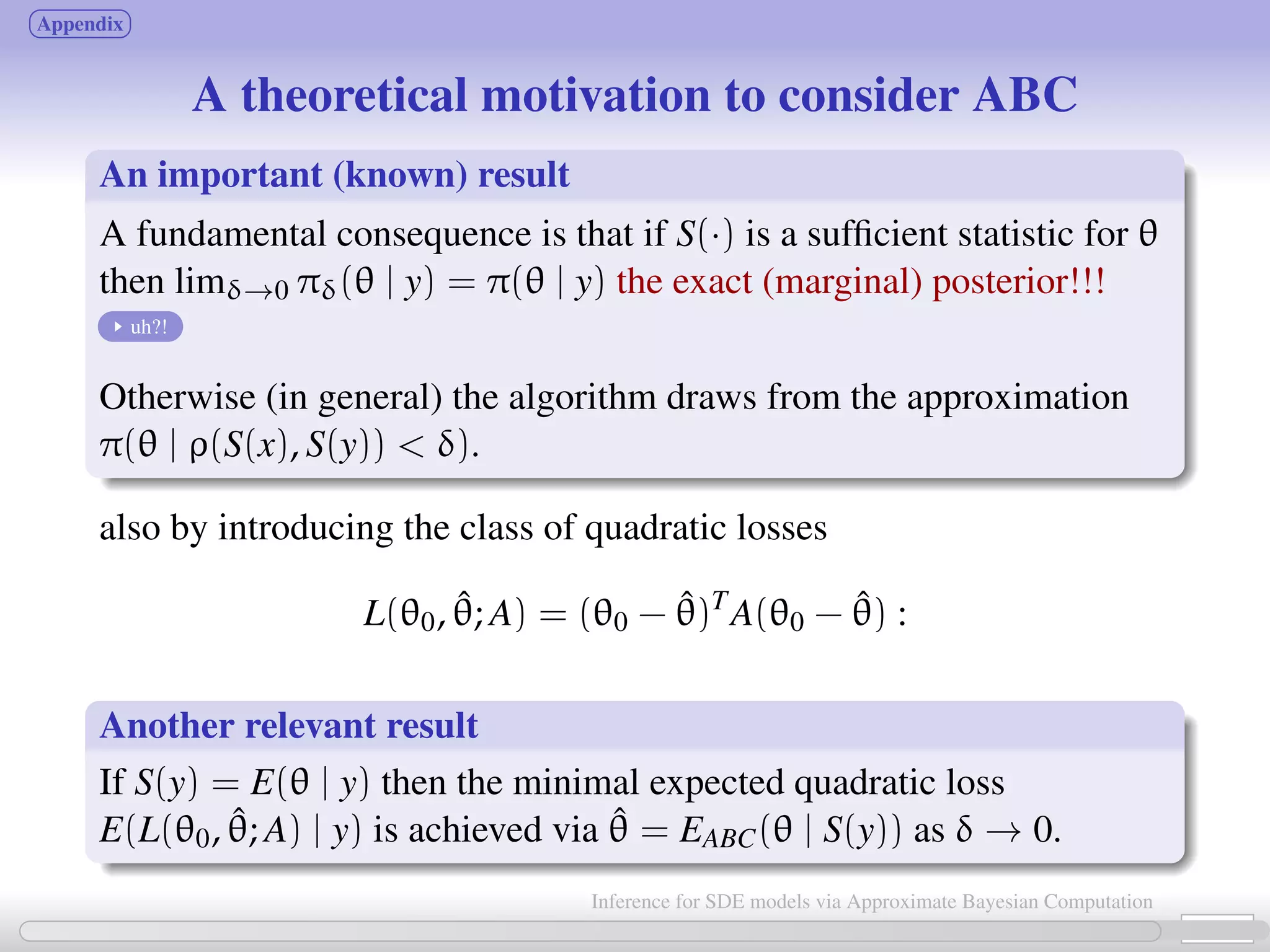
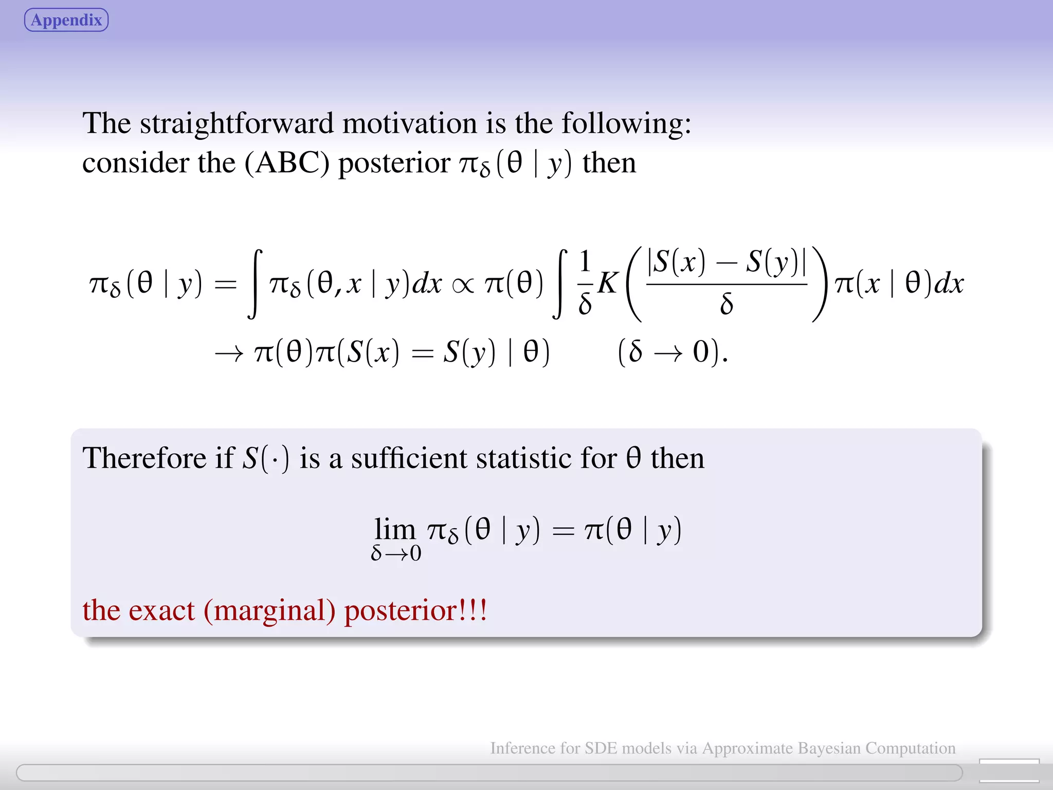
The previous algorithm generates a sequence {θr, xr} from the (ABC) posterior πδ(θ, xr | y). We only retain the {θr} which are thus from πδ(θ | y), the (marginal) ABC posterior of θ. In order to apply ABC methodology we are required to specify the statistic S(·) for θ. [Fearnhead Prangle 2012] (Classic result of Bayesian stats: for quadratic losses) the “optimal” choice of S(y) is given by S(y) = E(θ | y), the (unknown) posterior of θ. So Fearnhead Prangle propose a regression-based approach to determine S(·) (prior to MCMC start): for the jth parameter in θ fit the following linear regression models Sj(y) = Ê(θj|y) = ˆβ (j) 0 + ˆβ(j) η(y), j = 1, 2, ..., dim(θ) [e.g. Sj(y) = ˆβ (j) 0 + ˆβ(j) η(y) = ˆβ (j) 0 + ˆβ (j) 1 y0 + · · · + ˆβ (j) n yn] repeat the fitting separately for each θj. hopefully Sj(y) = ˆβ (j) 0 + ˆβ(j) η(y) will be “informative” for θj. 10 / 21 Inference for SDE models via Approximate Bayesian Computation

An example (run prior to MCMC ABC): 1. simulate from the prior θ ∼ π(θ) (not very efﬁcient...) 2. generate xsim ∼ π(x | θ ), then put ysim = xsim + ε repeat (1)-(2) many times to get the following matrices:     θ (1) 1 θ (1) 2 · · · θ (1) p θ (2) 1 θ (2) 2 · · · θ (2) p ...     ,     y (1) sim,t0 y (1) sim,t1 · · · y (1) sim,tn y (2) sim,t0 y (2) sim,t1 · · · y (2) sim,tn ... ... · · · ...     and for each column of the left matrix do a multivariate linear regression (or Lasso, or MARS,...)     θ (1) j θ (2) j ...     =     1 y (1) sim,t0 y (1) sim,t1 · · · y (1) sim,tn 1 y (2) sim,t0 y (2) sim,t1 · · · y (2) sim,tn ... ... · · · ...     × βj (j = 1, ..., p), and obtain an (hopefully almost sufﬁcient!) statistic for θj Sj(y) = ˆβ (j) 0 + ˆβ(j) η(y) = ˆβ (j) 0 + ˆβ (j) 1 y0+· · ·+ ˆβ(j) n yn ⇒ plug this into MCMC alg. 11 / 21 Inference for SDE models via Approximate Bayesian Computation

In some cases we have obtained better results (than with linear regression) using statistics based on: regression via MARS (multivariate adaptive regression splines [Friedman 1991]); Lasso-like estimation via glmnet [Friedman, Hastie, Tibshirani 2001]: estimates are found via ˆβ = argminβ 1 2 n i=0 (yi − p j=1 ηijβj)2 + γ p j=1 | βj | and the penality γ selected via cross validation methods (the one giving the smallest mean prediction error is selected). 12 / 21 Inference for SDE models via Approximate Bayesian Computation

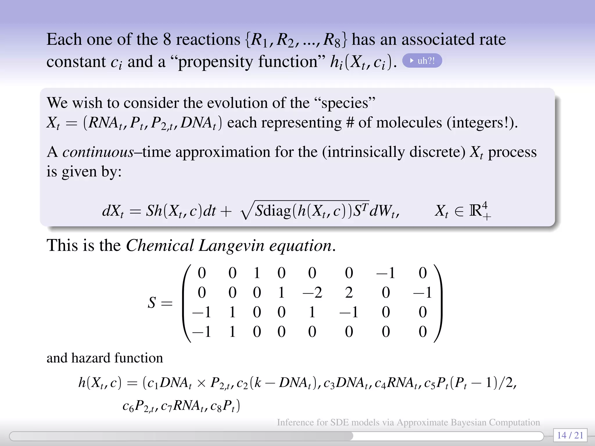
An application: Stochastic kinetic networks [also in Golightly-Wilkinson, 2010] Consider a set of reactions {R1, R2, ..., R8}: R1 : DNA + P2 → DNA · P2 R2 : DNA · P2 → DNA + P2 R3 : DNA → DNA + RNA R4 : RNA → RNA + P R5 : 2P → P2 (dimerization) R6 : P2 → 2P (dimerization) R7 : RNA → ∅ (degradation) R8 : P → ∅ (degradation) These reactions represent a simpliﬁed model for prokaryotic auto-regulation. “Reactants” are on the left side of →; “Products” are on the right side of →; There are several ways to simulate biochemical networks, e.g. the “exact” Gillespie algorithm (computationally intense for inferential purposes). Or by using a diffusion approximation ⇒ SDE. 13 / 21 Inference for SDE models via Approximate Bayesian Computation

Each one of the 8 reactions {R1, R2, ..., R8} has an associated rate constant ci and a “propensity function” hi(Xt, ci). uh?! We wish to consider the evolution of the “species” Xt = (RNAt, Pt, P2,t, DNAt) each representing # of molecules (integers!). A continuous–time approximation for the (intrinsically discrete) Xt process is given by: dXt = Sh(Xt, c)dt + Sdiag(h(Xt, c))STdWt, Xt ∈ R4 + This is the Chemical Langevin equation. S =     0 0 1 0 0 0 −1 0 0 0 0 1 −2 2 0 −1 −1 1 0 0 1 −1 0 0 −1 1 0 0 0 0 0 0     and hazard function h(Xt, c) = (c1DNAt × P2,t, c2(k − DNAt), c3DNAt, c4RNAt, c5Pt(Pt − 1)/2, c6P2,t, c7RNAt, c8Pt) 14 / 21 Inference for SDE models via Approximate Bayesian Computation

Simulation Study data D1 fully observed without error – all coordinates of {Xt} ∈ R4 + are observed; – yti ≡ Xti . – 50 measurements for each coordinate, n = 200 total observations. – we want to estimate θ = (c1, c2, ..., c8). data D2 fully observed with known error – all coordinates of {Xt} ∈ R4 + are observed; – yti = Xti + εti , εti ∼ N(0, σ2 εI); – we want to estimate θ = (c1, c2, ..., c8) (notice σε is known). D3 partially observed with unknown error - the DNAt coordinate is not observed ⇒ yti ∈ R3 + – want to estimate θ = (DNA0, c1, c2, ..., c8, σε). 15 / 21 Inference for SDE models via Approximate Bayesian Computation

0 5 10 15 20 25 30 35 40 45 50 0 2 4 6 8 10 12 14 16 time Xt Figure: Data D1 connected with lines. RNA (◦), P (∗), P2 ( ), DNA (+). 16 / 21 Inference for SDE models via Approximate Bayesian Computation

In all 3 cases a chain having 3,000,000 elements is generated (∼15 hrs with Matlab). Priors: log cj ∼ U(−3, 0) and log DNA0 ∼ U(0, 2.3) (when needed). True values D1 D2 D3 DNA0 5 — — 3.110 [1.441, 6.526] c1 0.1 0.074 0.074 0.074 [0.057, 0.097] [0.055, 0.099] [0.056, 0.097] c2 0.7 0.521 0.552 0.536 [0.282, 0.970] [0.294, 1.029] [0.345, 0.832] c1/c2 0.143 0.142 0.135 0.138 c3 0.35 0.216 0.214 0.244 [0.114, 0.4081] [0.109, 0.417] [0.121, 0.492] c4 0.2 0.164 0.168 0.174 [0.088, 0.308] [0.088, 0.312] [0.089, 0.331] c5 0.1 0.088 0.088 0.087 [0.070, 0.112] [0.069, 0.114] [0.063, 0.120] c6 0.9 0.352 0.355 0.379 [0.139, 0.851] [0.136, 0.880] [0.147, 0.937] c5/c6 0.111 0.250 0.248 0.228 c7 0.3 0.158 0.158 0.157 [0.113, 0.221] [0.108, 0.229] [0.103, 0.240] c8 0.1 0.160 0.169 0.165 [0.098, 0.266] [0.097, 0.286] [0.091, 0.297] σε 1.414 — — 0.652 [0.385, 1.106] 17 / 21 Inference for SDE models via Approximate Bayesian Computation

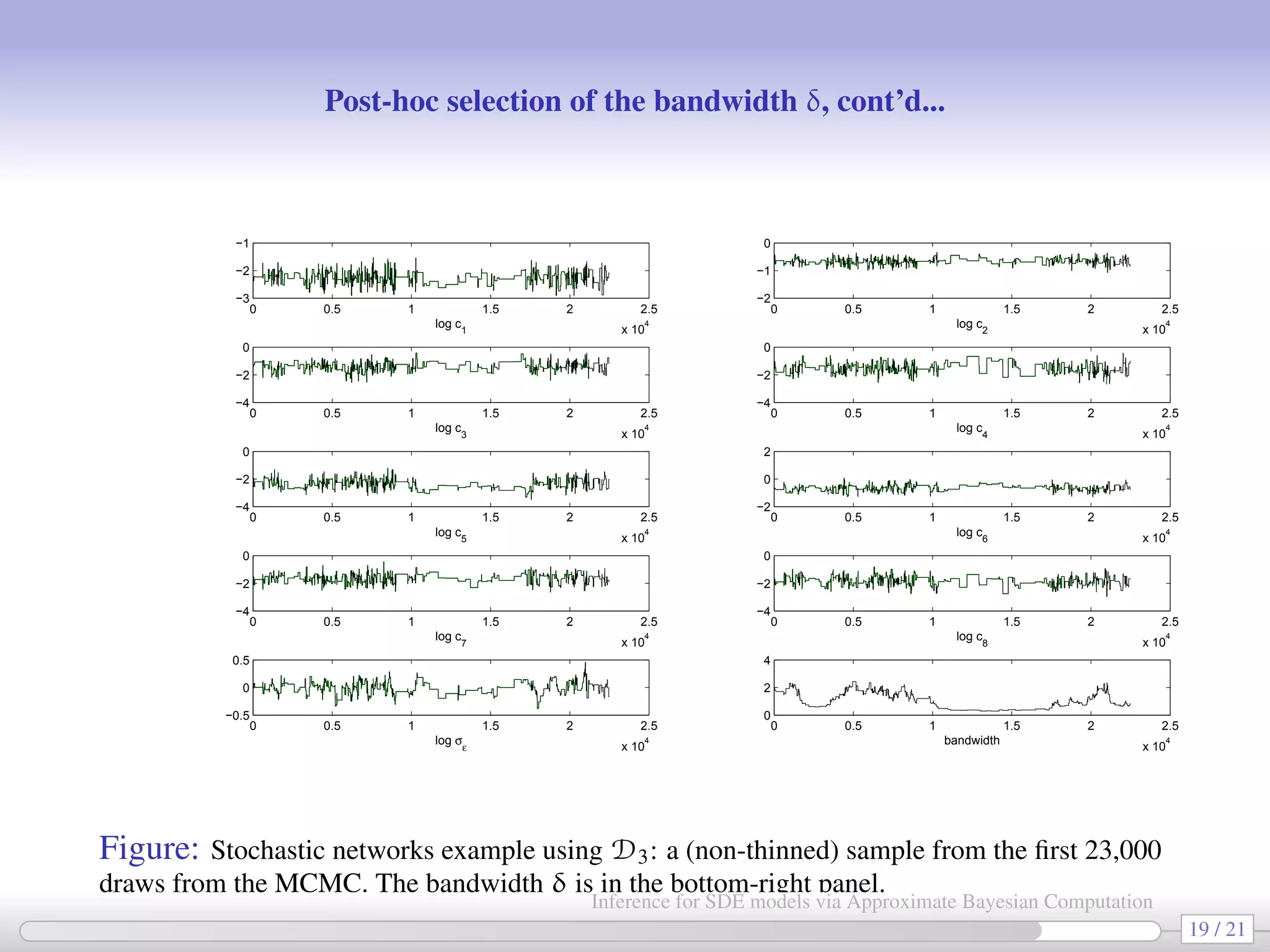
HOWTO: post-hoc selection of δ (the “precision” parameter) [Bortot et al. 2007] As previously explained, during the MCMC we let δ vary (according to a MRW): at rth iteration δr = δr−1 + ∆, with ∆ ∼ N(0, ν2 ). After the end of the MCMC we have a sequence {θr, δr}r=0,1,2... and for each parameter {θj,r}r=0,1,2... we produce a plot like the following (e.g. log c3 vs δ): 0 0.5 1 1.5 2 2.5 3 3.5 4 −2.5 −2 −1.5 −1 −0.5 0 bandwidth 18 / 21 Inference for SDE models via Approximate Bayesian Computation

Post-hoc selection of the bandwidth δ, cont’d... 0 0.5 1 1.5 2 2.5 x 10 4 −3 −2 −1 log c1 0 0.5 1 1.5 2 2.5 x 10 4 −2 −1 0 log c2 0 0.5 1 1.5 2 2.5 x 10 4 −4 −2 0 log c3 0 0.5 1 1.5 2 2.5 x 10 4 −4 −2 0 log c4 0 0.5 1 1.5 2 2.5 x 10 4 −4 −2 0 log c5 0 0.5 1 1.5 2 2.5 x 10 4 −2 0 2 log c6 0 0.5 1 1.5 2 2.5 x 10 4 −4 −2 0 log c7 0 0.5 1 1.5 2 2.5 x 10 4 −4 −2 0 log c8 0 0.5 1 1.5 2 2.5 x 10 4 −0.5 0 0.5 log σε 0 0.5 1 1.5 2 2.5 x 10 4 0 2 4 bandwidth Figure: Stochastic networks example using D3: a (non-thinned) sample from the ﬁrst 23,000 draws from the MCMC. The bandwidth δ is in the bottom-right panel. 19 / 21 Inference for SDE models via Approximate Bayesian Computation

Post-hoc selection of the bandwidth δ, cont’d... Therefore in practice: we ﬁlter out of the analyses those draws {θr}r=0,1,2,... corresponding to “large” δ, for statistical precision; we retain only those {θr}r=0,1,2,... corresponding to a low δ (but not too low, because of previous considerations). in the example we retain {θr; δr 1.5}. PRO: this is useful as it allows an ex-post selection of δ, i.e. we do not need to know in advance a suitable value for δ. CON: by ﬁltering out some of the draws, a disadvantage of the approach is the need to run very long MCMC simulations in order to have enough “material” on which to base our posterior inference. PRO: also notice that by letting δ vary we are effectively considering a global optimization method (similar to simulated tempering tempered transitions). 20 / 21 Inference for SDE models via Approximate Bayesian Computation

Conclusions Approximate Bayesian Computation allows inference from a wide class of models which would otherwise be unavailable. ..but it’s not a silver bullet! construct the statistics S(·) by simulating parameters from the prior is highly inefﬁcient; long simulations are needed as a price to be paid in any algorithm that avoids likelihood calculations (∼ millions of MCMC iterations, but this is not necessarily very time consuming as we avoid the most computationally intense part, that is likelihood calculation!); Paper: P. (2013) http://arxiv.org/abs/1204.5459 a general MATLAB implementation for fully and partially observed SDEs is available at https://sourceforge.net/projects/abc-sde/. Thank you! 21 / 21 Inference for SDE models via Approximate Bayesian Computation

Appendix Proof that the basic ABC algorithm works The proof is straightforward. We know that an accepted draw (θ , x ) produced by the algorithm is such that (i) θ ∼ π(θ), and (ii) such that x = xobs, where x ∼ π(x | θ ). Thus let’s call f(θ ) the (unknown) marginal density for such θ , then because of (i) and (ii) f(θ ) ∝ x π(θ )π(x|θ )Ixobs (x) = x=xobs π(θ , x) ∝ π(θ|xobs). Therefore θ ∼ π(θ|xobs). 22 / 21 Inference for SDE models via Approximate Bayesian Computation

Appendix A theoretical motivation to consider ABC An important (known) result A fundamental consequence is that if S(·) is a sufﬁcient statistic for θ then limδ→0 πδ(θ | y) = π(θ | y) the exact (marginal) posterior!!! uh?! Otherwise (in general) the algorithm draws from the approximation π(θ | ρ(S(x), S(y)) δ). also by introducing the class of quadratic losses L(θ0, ˆθ; A) = (θ0 − ˆθ)T A(θ0 − ˆθ) : Another relevant result If S(y) = E(θ | y) then the minimal expected quadratic loss E(L(θ0, ˆθ; A) | y) is achieved via ˆθ = EABC(θ | S(y)) as δ → 0. 23 / 21 Inference for SDE models via Approximate Bayesian Computation

Appendix Some remarks on SysBio concepts a “propensity function” hi(Xt, ci) gives the overall hazard of a type i reaction occurring, that is the probability of a type i reaction occurring in the time interval (t, t + dt] is hi(Xt, ci)dt. a “conservation law” (from redundant rows in S): DNA · P2 + DNA = k. In a stoichiometry matrix S reactants appear as negative values and products appear as positive values. 25 / 21 Inference for SDE models via Approximate Bayesian Computation

Appendix Choice of kernel function We follow Fearnhead-Prangle(2012): we consider bounded kernels K(·) 1; specifically we use the uniform kernel K(z) returning 1 when zT Az c and 0 otherwise. In our case z = (S(ysim) − S(y))/δ and A is chosen to be a p × p diagonal matrix defining the relative weighting of the parameters in the loss function. The uniform kernel is defined on a region zT Az bounded by a volume c, with c = Vp|A|1/p , where Vp = π−1 [Γ(p/2)p/2]2/p and p = dim(θ); such c is the unique value producing a valid probability density function K i.e. such that the volume of the region zT Az c equals 1. 26 / 21 Inference for SDE models via Approximate Bayesian Computation

Inference for stochastic differential equations via approximate Bayesian computation

More Related Content

What's hot

Viewers also liked

Similar to Inference for stochastic differential equations via approximate Bayesian computation

More from Umberto Picchini

Recently uploaded

Inference for stochastic differential equations via approximate Bayesian computation