Download as PDF, PPTX

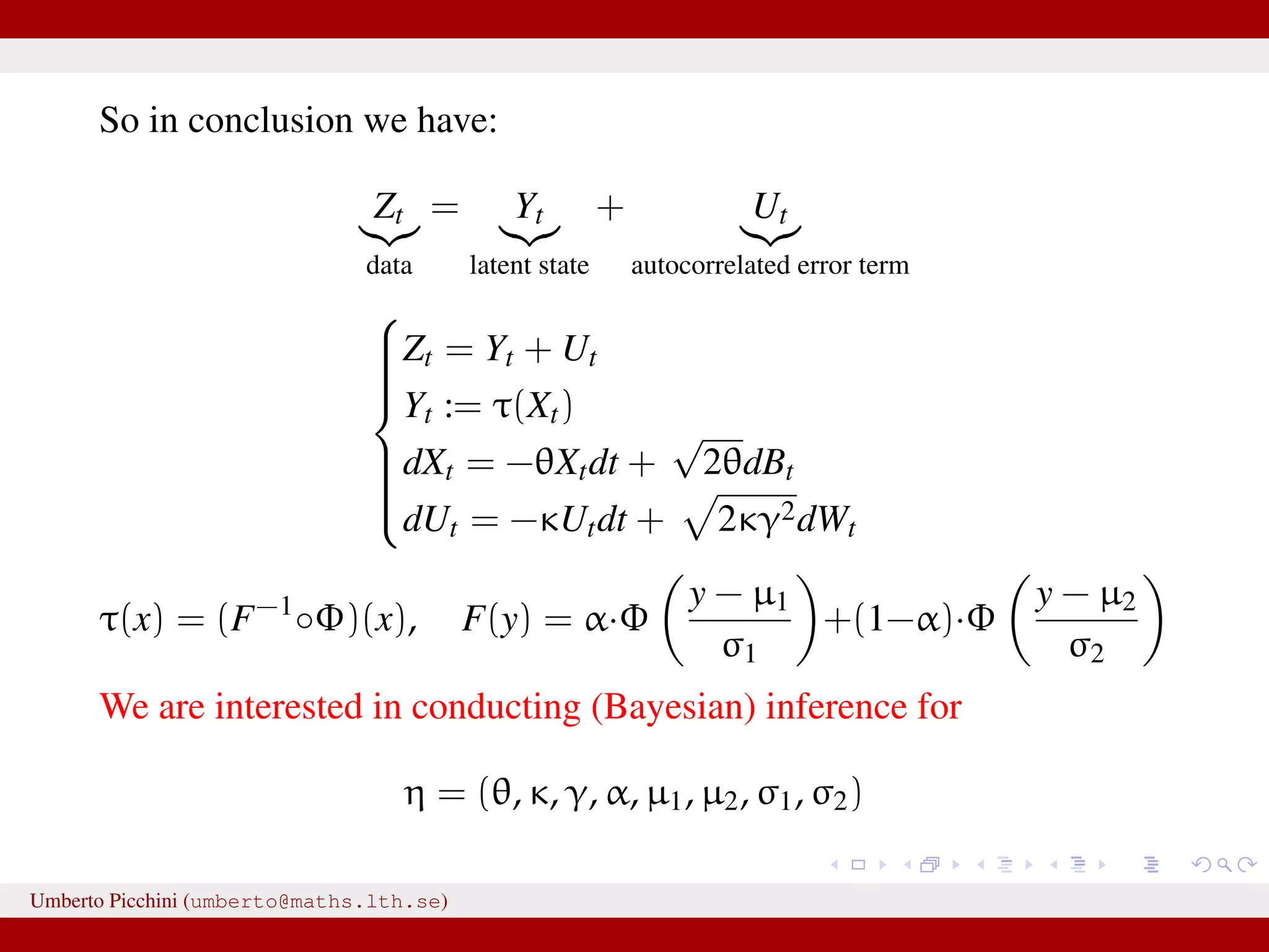
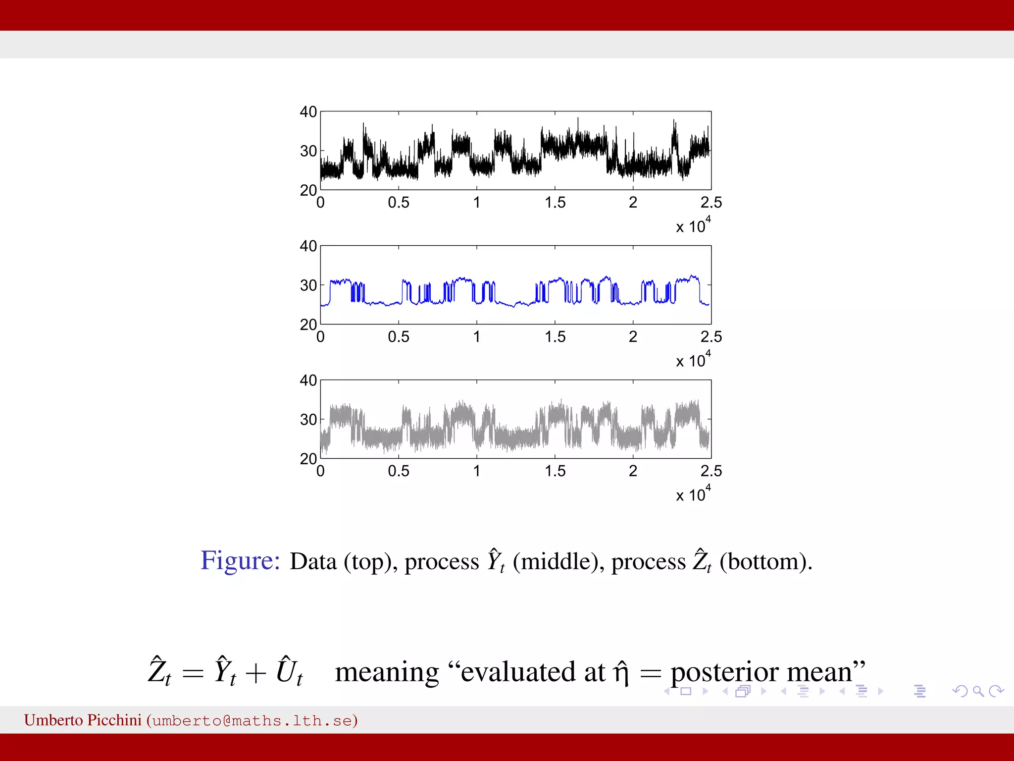
![Forman and Sørensen [2013] proposed to consider sums of diffusions:1 Zt observable process = Yt latent state + Ut autocorrelated error term they considered diffusion processes to modelize both Yt and Ut they found i.i.d. errors where not really giving satisfactory results. So let’s introduce some autocorrelation: dUt = −κUtdt + 2κγ2dWt, U0 = 0 a zero mean Ornstein-Uhlenbeck process with stationary variance γ2 and autocorrelation ρU(t) = e−κt. Here dWt ∼ N(0, dt). 1 Forman and Sørensen, A transformation approach to modelling multi-modal diffusions. J. Statistical Planning and Inference. 2014. Umberto Picchini (umberto@maths.lth.se)](https://image.slidesharecdn.com/abcprotein-160217214818/75/Accelerated-approximate-Bayesian-computation-with-applications-to-protein-folding-data-8-2048.jpg)

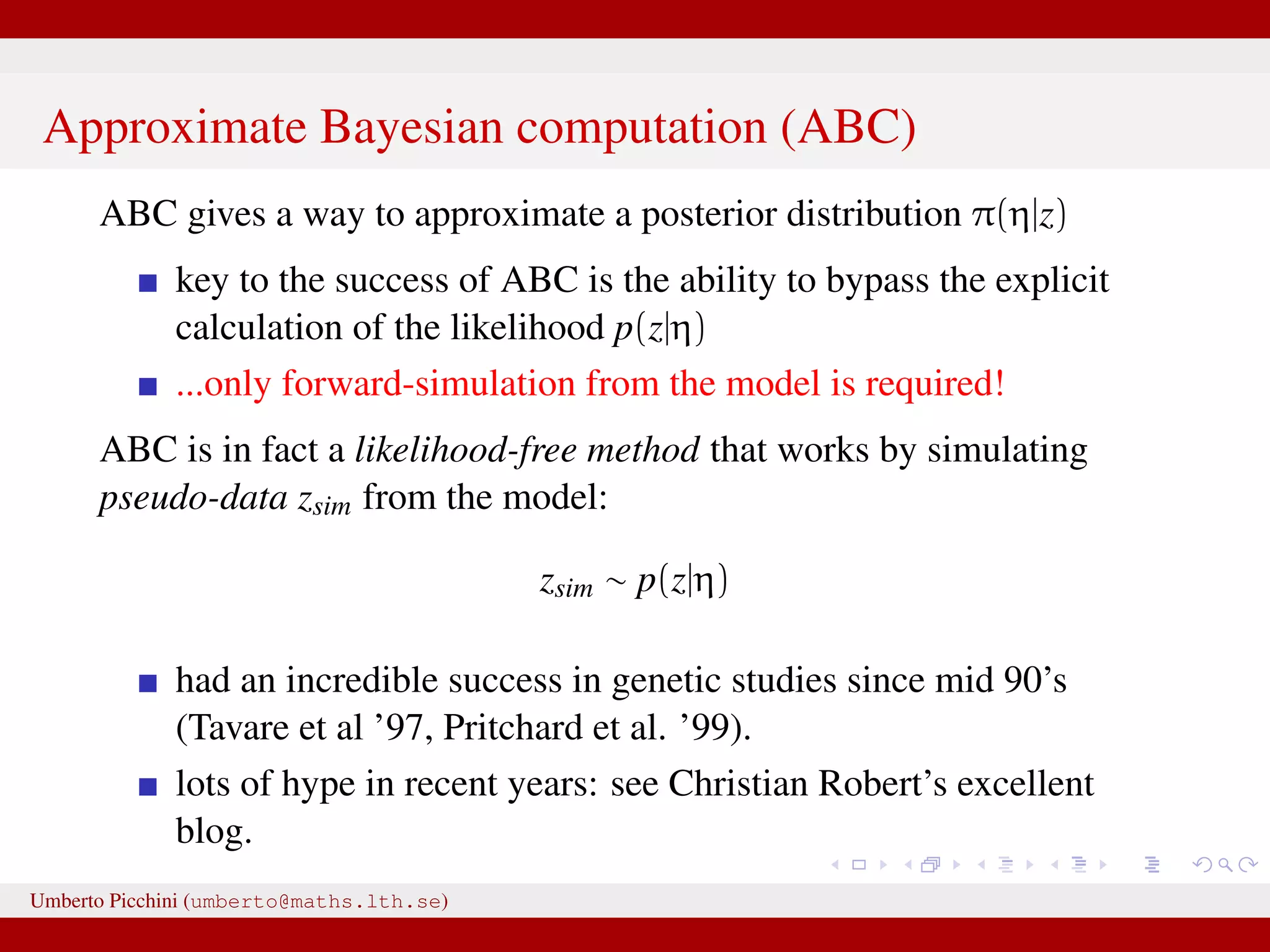
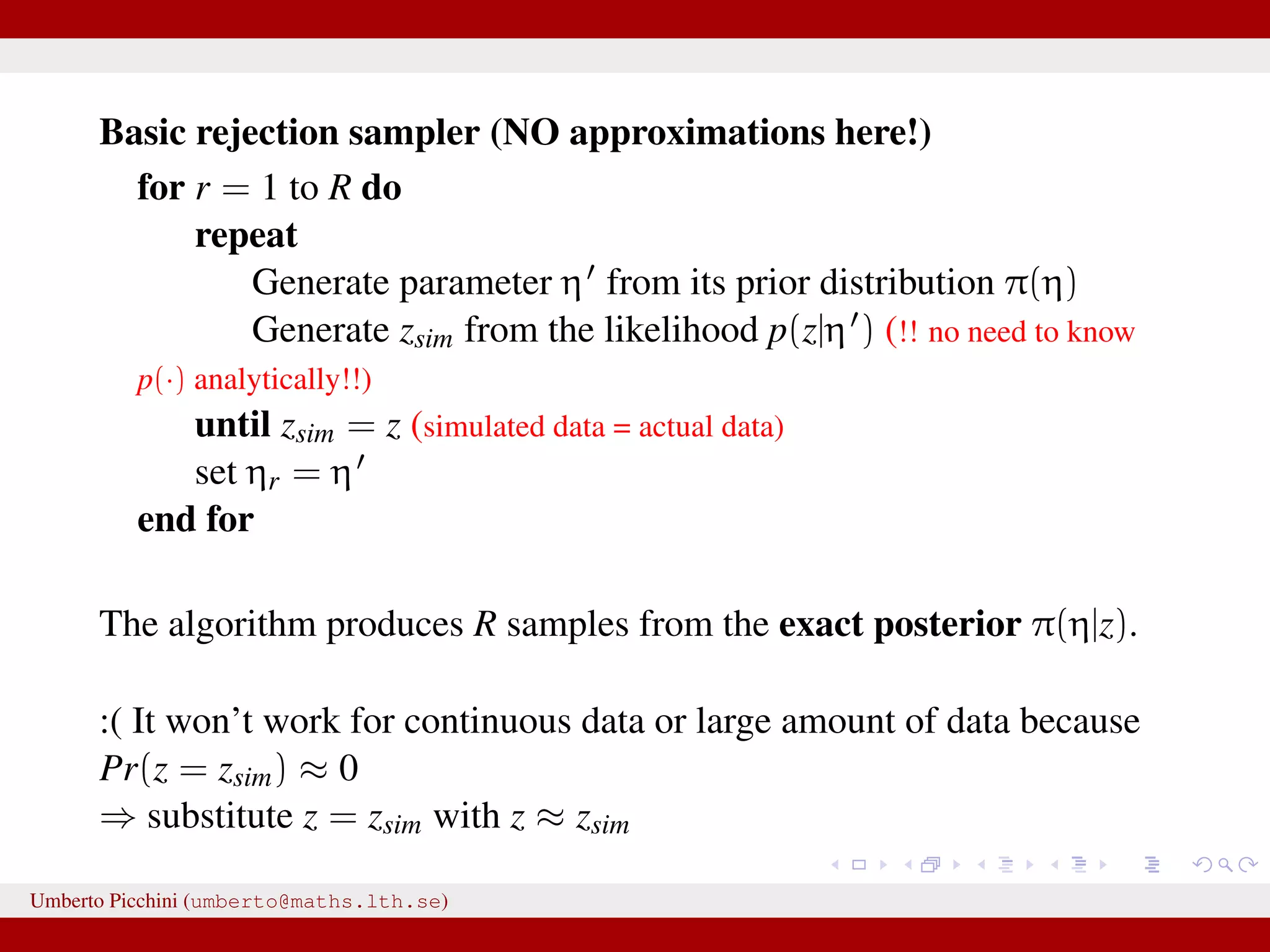
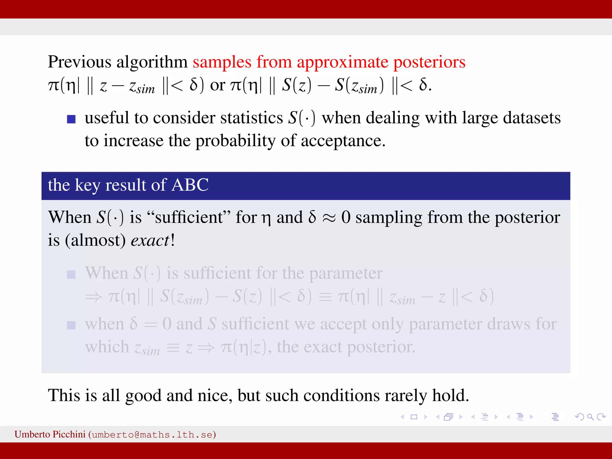
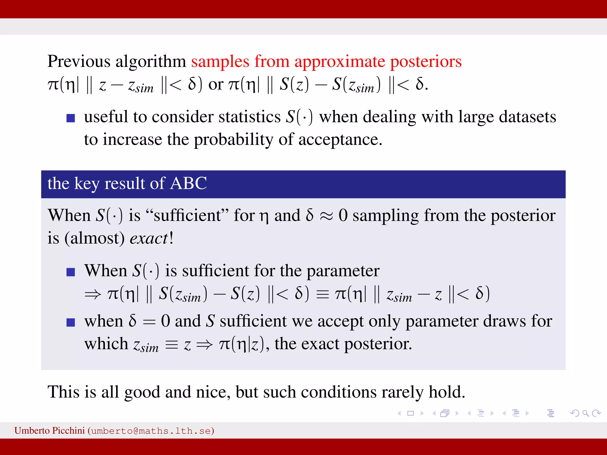
![...⇒ substitute z = zsim with z ≈ zsim Introduce some distance z − zsim to measure proximity of zsim and data z [Pritchard et al. 1999]. Introduce a tolerance value δ > 0. An ABC rejection sampler: for r = 1 to R do repeat Generate parameter η from its prior distribution π(η) Generate zsim from the likelihood p(z|η ) until z − zsim < δ [or alternatively S(z) − S(zsim) < δ] set ηr = η end for for some “summary statistics” S(·). Umberto Picchini (umberto@maths.lth.se)](https://image.slidesharecdn.com/abcprotein-160217214818/75/Accelerated-approximate-Bayesian-computation-with-applications-to-protein-folding-data-17-2048.jpg)
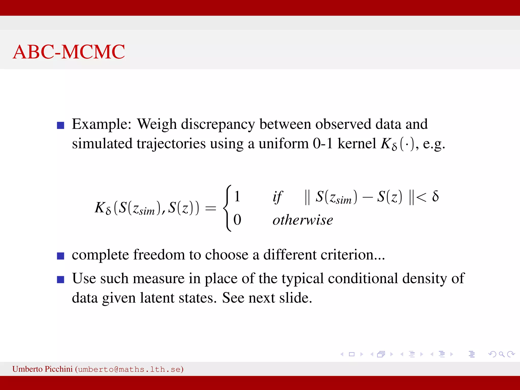
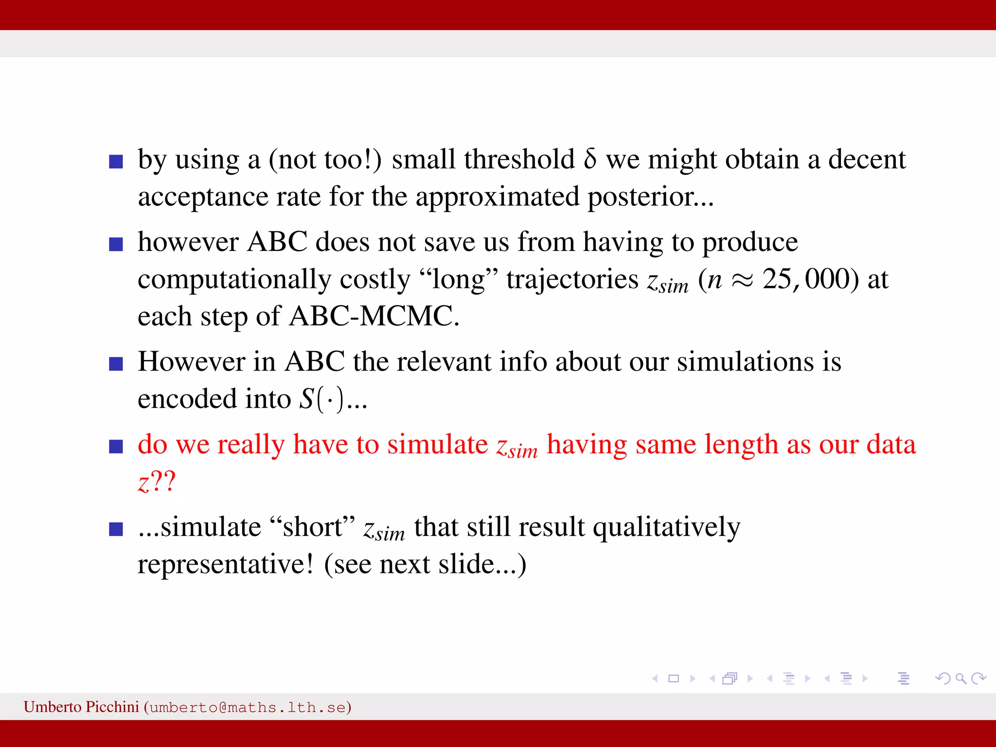
![a central problem is how to choose the statistics S(·): outside the exponential family we typically cannot derive sufficient statistics. [A key work to obtain “semi-automatically” statistics is Fearnhead-Prangle ’12 (discussion paper on JRSS-B. Very much recommended.)] substitute with the loose concept of informative (enough) statistic then choose a small (enough) threshold δ. We now go back to our model and (large) data. We propose some trick to accelerate the inference. We will use an ABC within MCMC approach (ABC-MCMC). Umberto Picchini (umberto@maths.lth.se)](https://image.slidesharecdn.com/abcprotein-160217214818/75/Accelerated-approximate-Bayesian-computation-with-applications-to-protein-folding-data-20-2048.jpg)
![a central problem is how to choose the statistics S(·): outside the exponential family we typically cannot derive sufficient statistics. [A key work to obtain “semi-automatically” statistics is Fearnhead-Prangle ’12 (discussion paper on JRSS-B. Very much recommended.)] substitute with the loose concept of informative (enough) statistic then choose a small (enough) threshold δ. We now go back to our model and (large) data. We propose some trick to accelerate the inference. We will use an ABC within MCMC approach (ABC-MCMC). Umberto Picchini (umberto@maths.lth.se)](https://image.slidesharecdn.com/abcprotein-160217214818/75/Accelerated-approximate-Bayesian-computation-with-applications-to-protein-folding-data-21-2048.jpg)


![Results after 2 millions ABC-MCMC iterations. Acceptance rate of 1% and 6 hrs computation with MATLAB on a common pc desktop. Table: Protein folding data experiment: posterior means from the ABC-MCMC output and 95% posterior intervals. ABC posterior means log θ –6.454 [–6.898,-5.909] log κ –0.651 [–1.424,0.246] log γ 0.071 [–0.313,0.378] log µ1 3.24 [3.22,3.26] log µ2 3.43 [3.39,3.45] log σ1 –0.959 [–2.45,0.38] log σ2 –0.424 [–2.26,0.76] log α –0.663 [–1.035,–0.383] Umberto Picchini (umberto@maths.lth.se)](https://image.slidesharecdn.com/abcprotein-160217214818/75/Accelerated-approximate-Bayesian-computation-with-applications-to-protein-folding-data-34-2048.jpg)

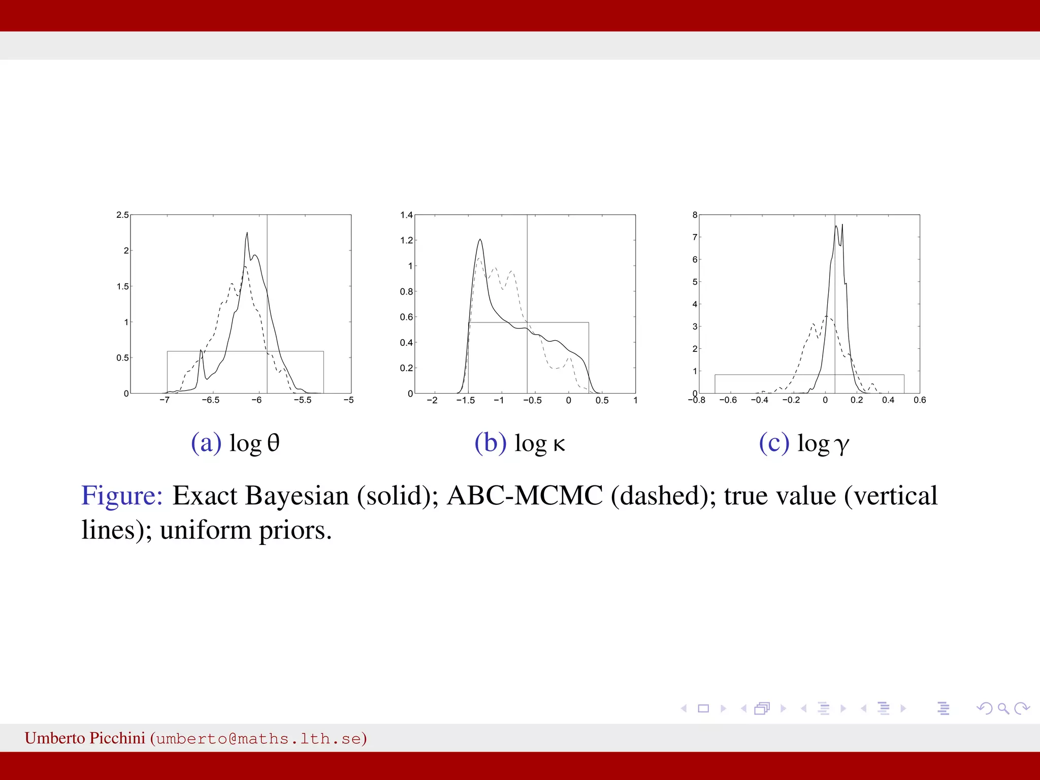
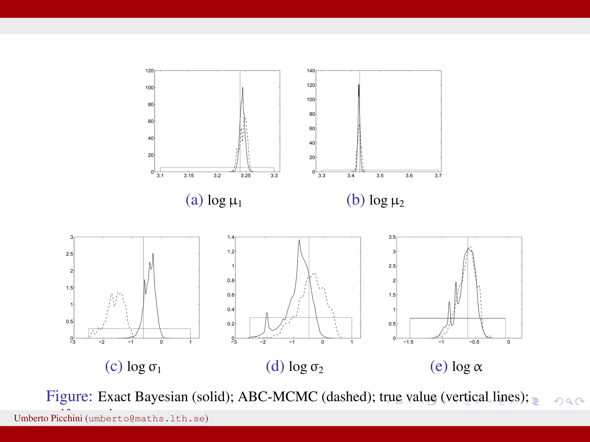
![Comparison ABC-MCMC (*) vs exact Bayes (pMCMC) True value θ 0.0027 0.0023 [0.0013,0.0041] 0.0024∗ [0.0013,0.0039] κ 0.538 0.444 [0.349,0.558] 0.553∗ [0.386,0.843] γ 1.063 1.040 [0.943,1.158] 0.982∗ [0.701,1.209] µ1 25.52 25.68 [25.08,26.61] 25.72∗ [25.10,26.71] µ2 30.92 32.12 [29.15,35.42] 32.17∗ [29.46,34.96] σ1 0.540 0.421 [0.203,0.844] 0.523∗ [0.248,0.972] σ2 0.624 0.502 [0.232,1.086] 0.511∗ [0.249,1.041] α 0.537 0.510 [0.345,0.755] 0.508∗ [0.346,0.721] Umberto Picchini (umberto@maths.lth.se)](https://image.slidesharecdn.com/abcprotein-160217214818/75/Accelerated-approximate-Bayesian-computation-with-applications-to-protein-folding-data-37-2048.jpg)


![Generation of δ’s 0 0.5 1 1.5 2 2.5 x 10 5 0 0.2 0.4 0.6 0.8 Here we generate a chain for log δ using a (truncated) Gaussian random walk with support (−∞, log δmax]. We let log δmax decrease during the simulation. Umberto Picchini (umberto@maths.lth.se)](https://image.slidesharecdn.com/abcprotein-160217214818/75/Accelerated-approximate-Bayesian-computation-with-applications-to-protein-folding-data-49-2048.jpg)
![HOWTO: post-hoc selection of δ (the “precision” parameter) [Bortot et al. 2007] During ABC-MCMC we let δ vary (according to a MRW): at rth iteration δr = δr−1 + ∆, with ∆ ∼ N(0, ν2 ). After the end of the MCMC we have a sequence {θr, δr}r=0,1,2... and for each parameter {θj,r}r=0,1,2... we produce a plot of the parameter chain vs δ: 0 0.5 1 1.5 2 2.5 3 3.5 4 −2.5 −2 −1.5 −1 −0.5 0 bandwidth Umberto Picchini (umberto@maths.lth.se)](https://image.slidesharecdn.com/abcprotein-160217214818/75/Accelerated-approximate-Bayesian-computation-with-applications-to-protein-folding-data-50-2048.jpg)

This document discusses the application of Approximate Bayesian Computation (ABC) methods to accelerate inference for protein folding models, highlighting the challenges faced in traditional Bayesian inference due to large datasets. It introduces models based on stochastic processes and emphasizes the use of summary statistics to improve computational efficiency. The document also details a proposed ABC-MCMC approach that combines these techniques to handle complex stochastic models effectively.