Downloaded 28 times

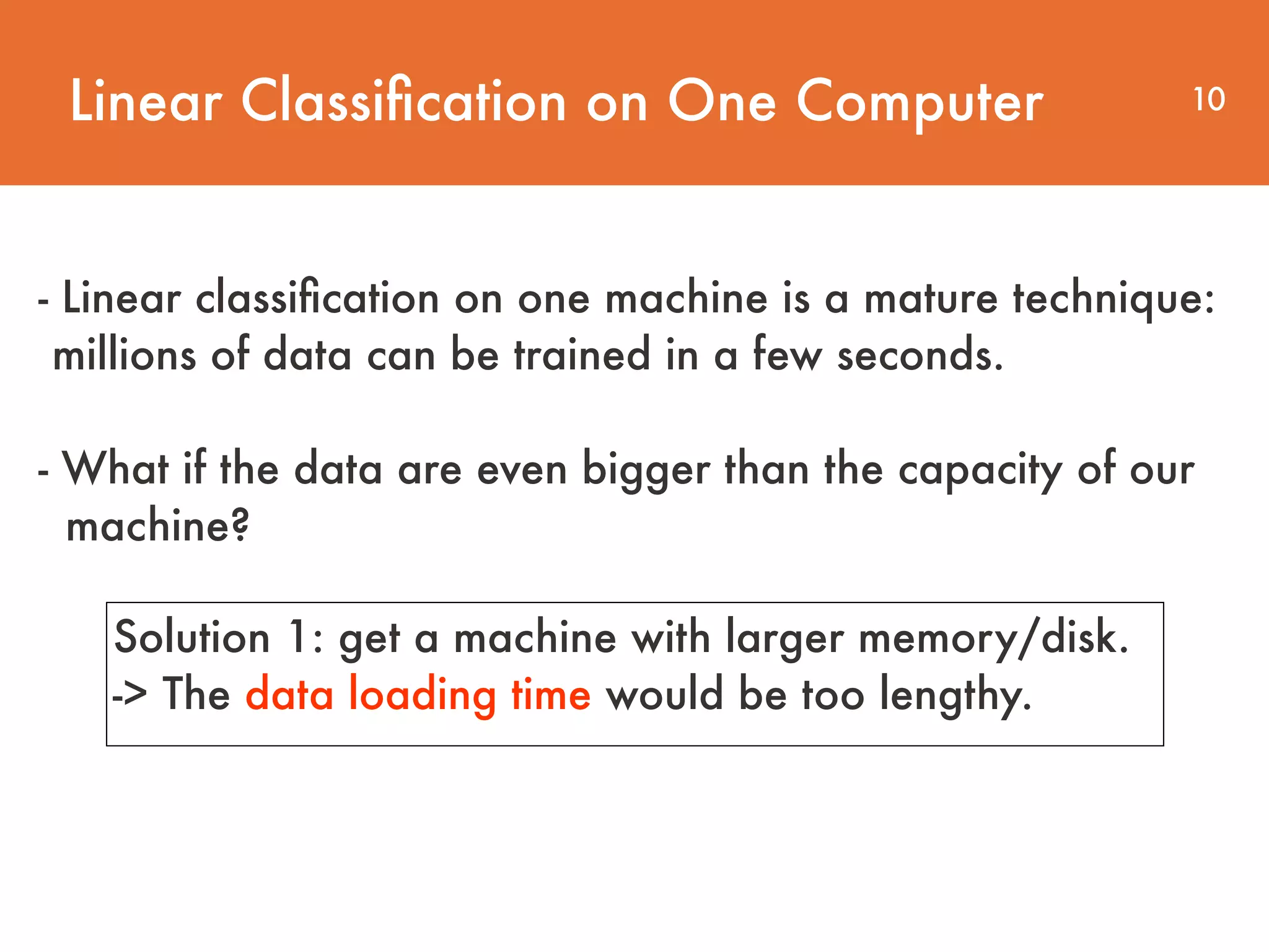
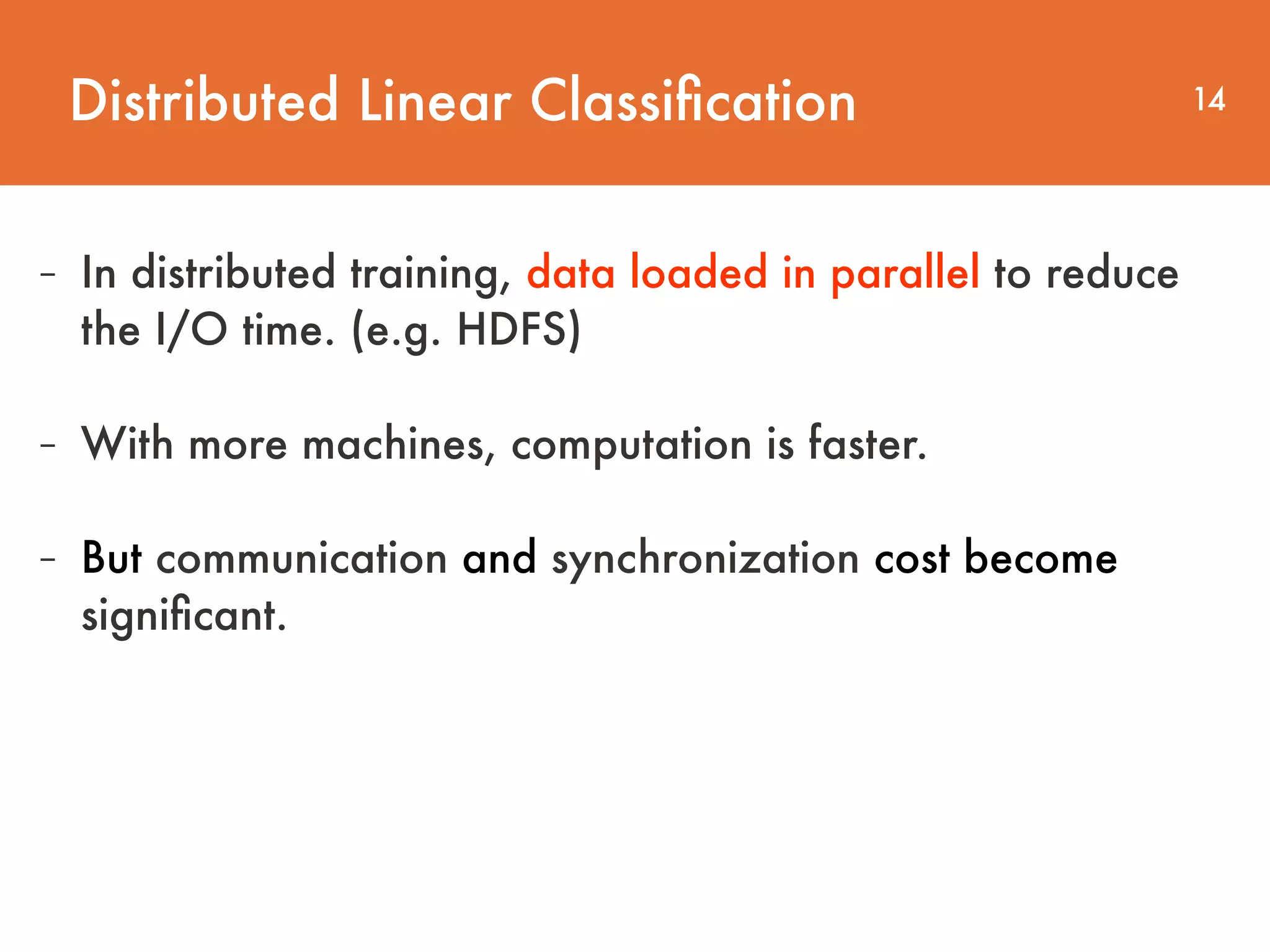
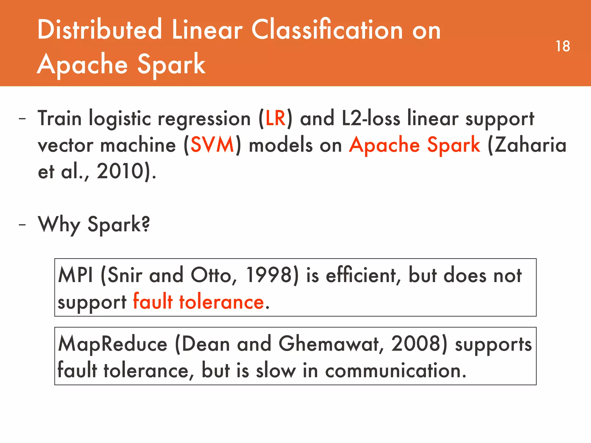
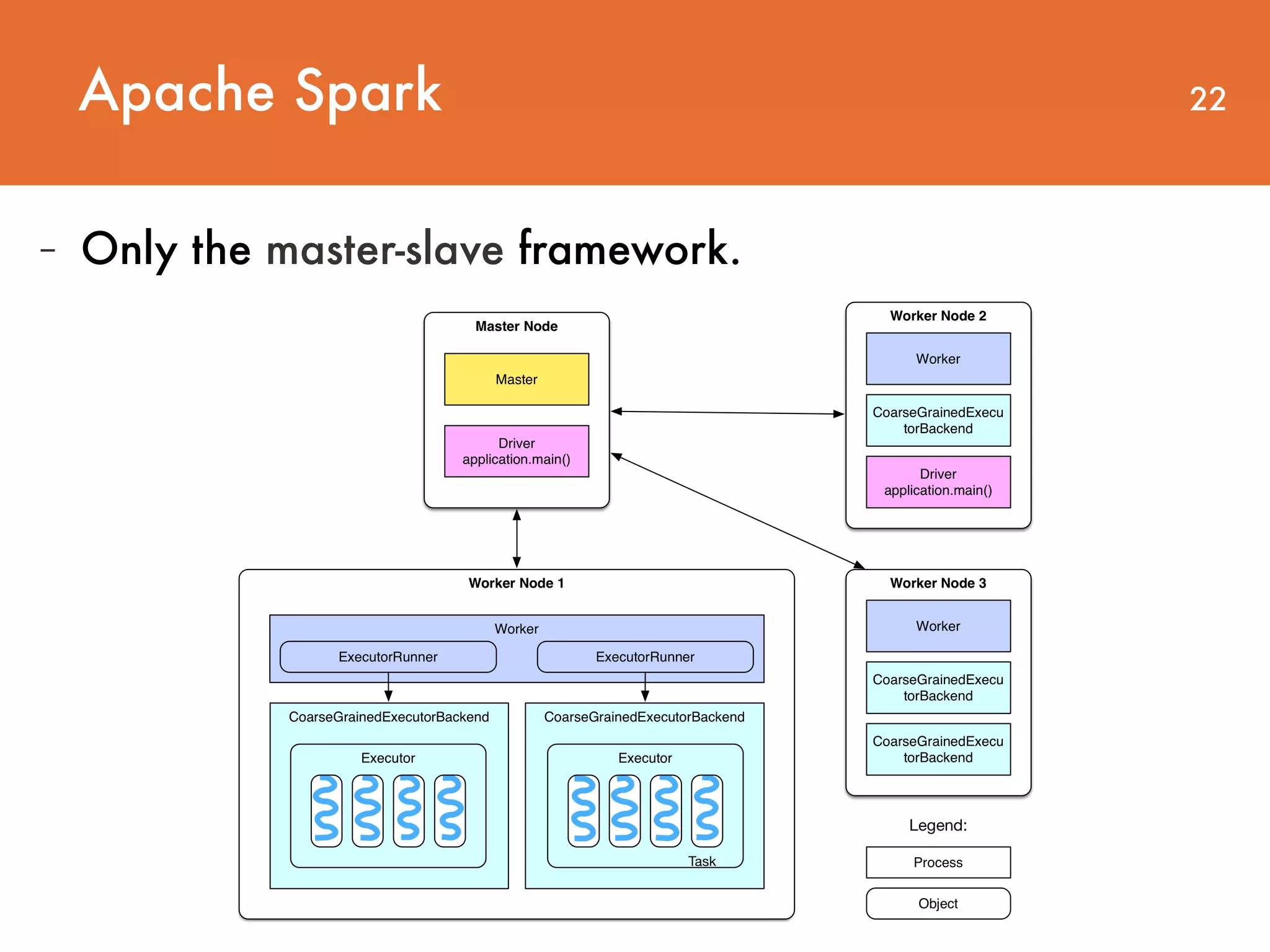
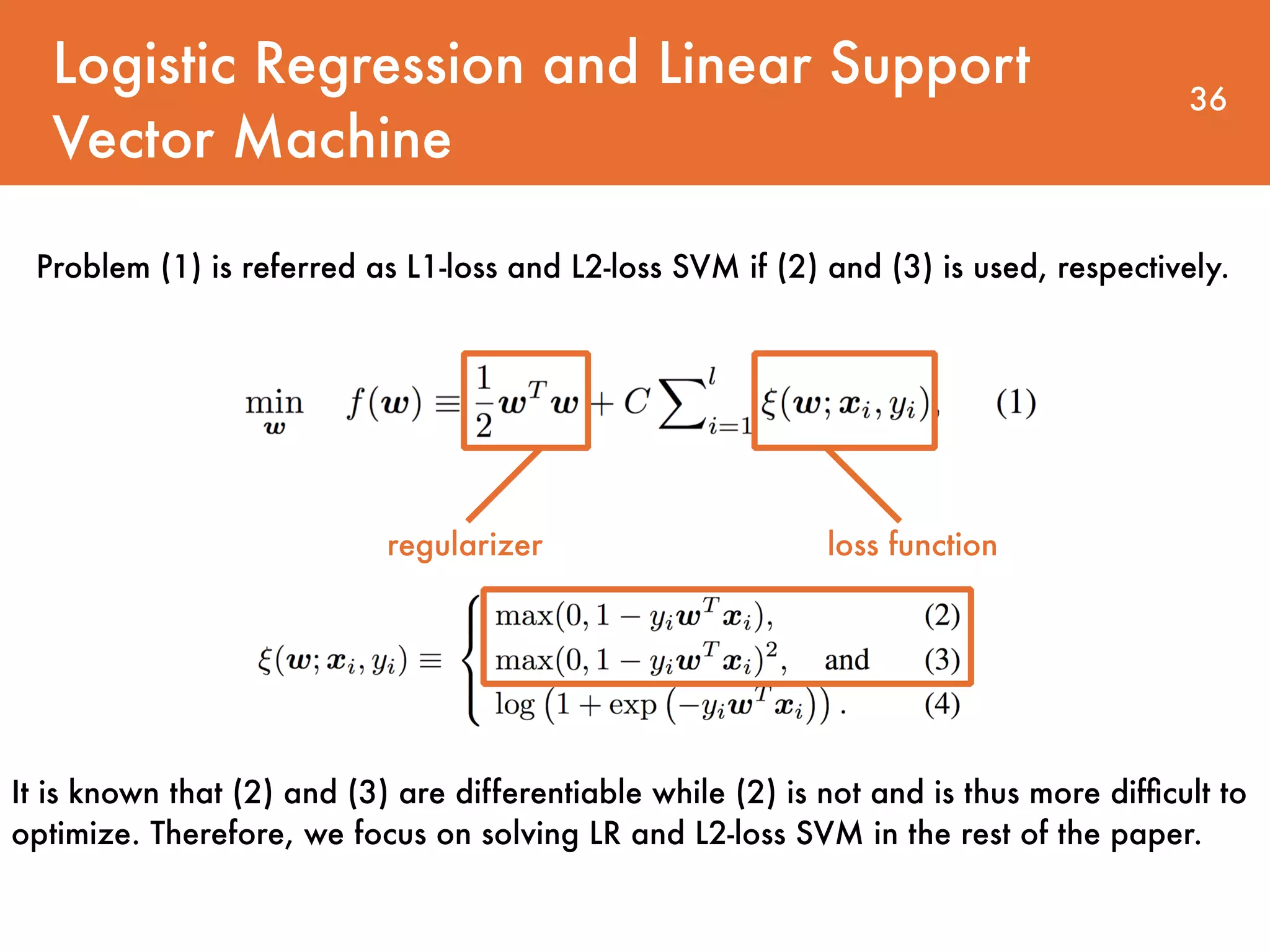
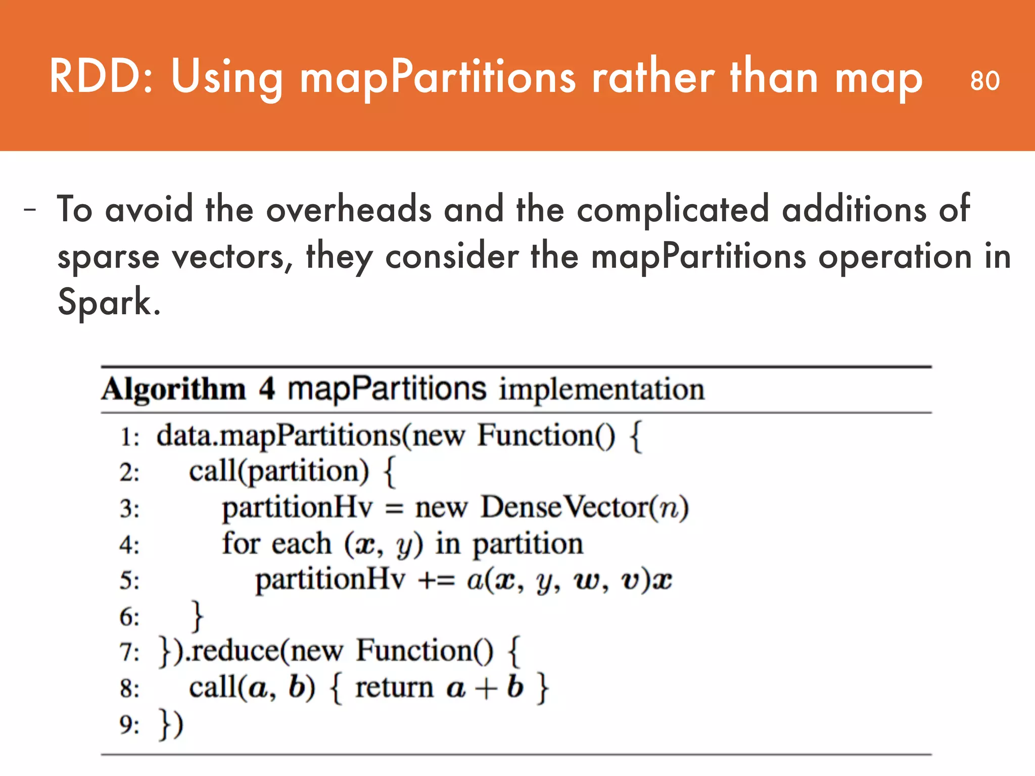
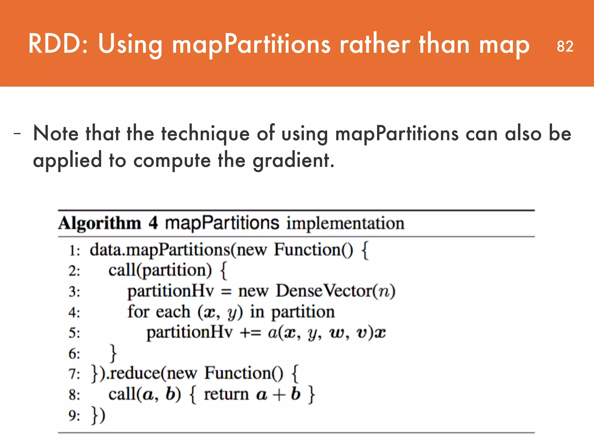
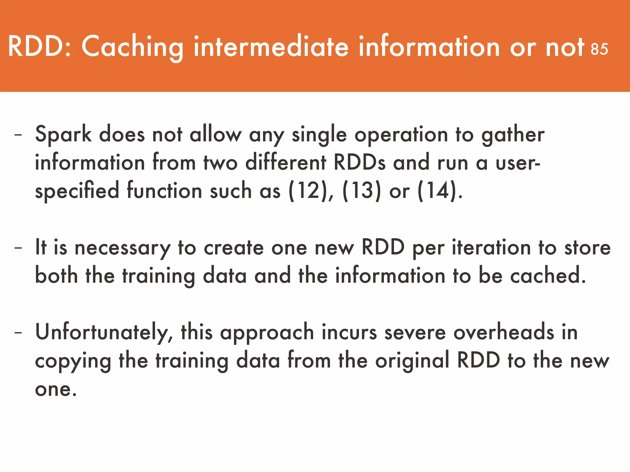
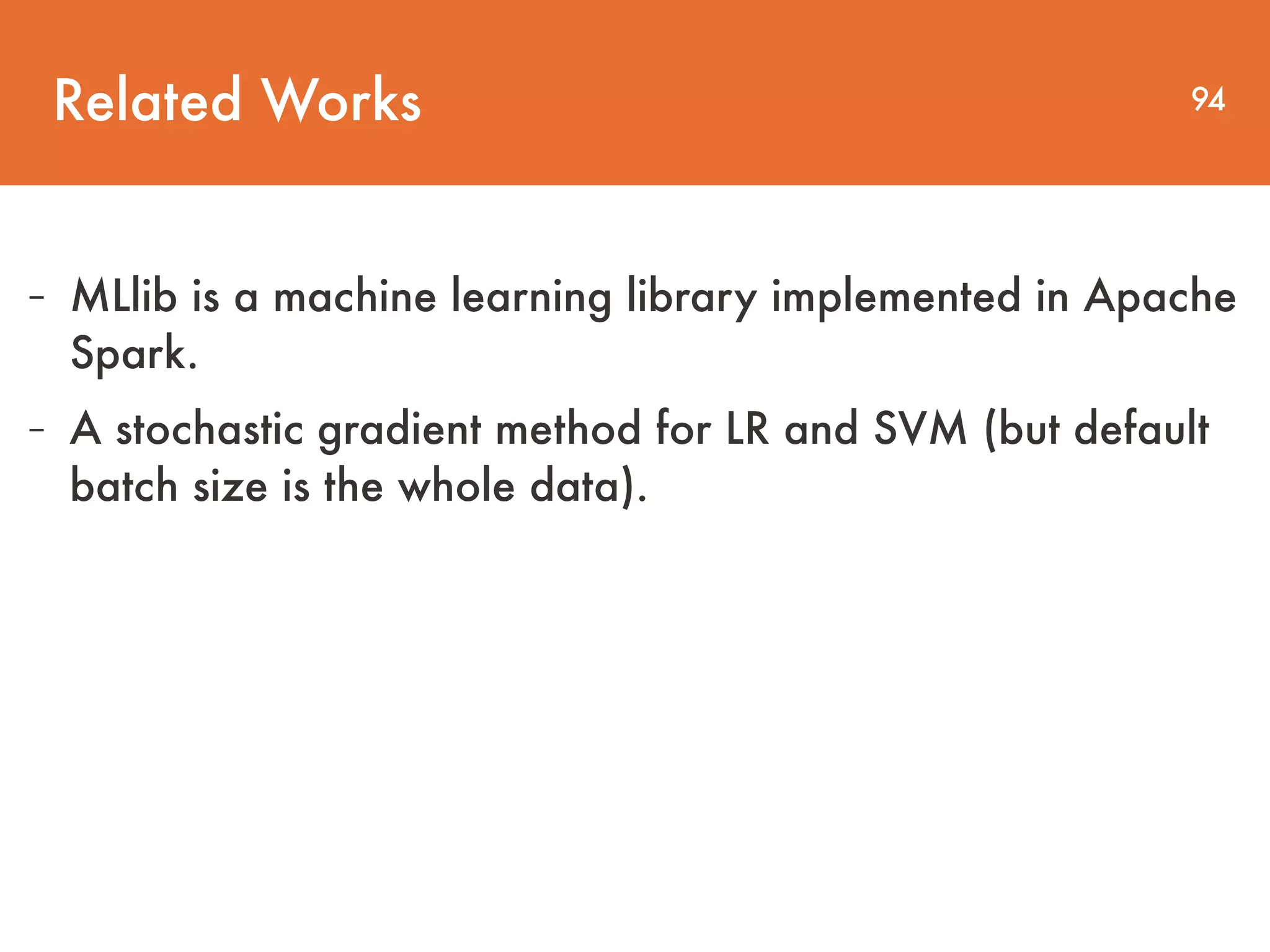
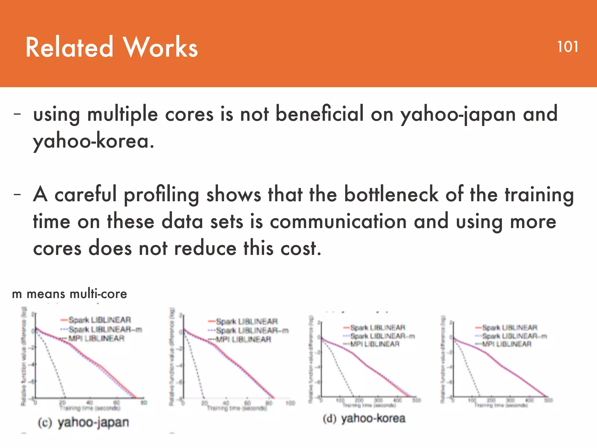
![Apache Spark (skip) 29 package org.apache.spark.examples import java.util.Random import org.apache.spark.{SparkConf, SparkContext} import org.apache.spark.SparkContext._ /** * Usage: GroupByTest [numMappers] [numKVPairs] [valSize] [numReducers] */ object GroupByTest { def main(args: Array[String]) { val sparkConf = new SparkConf().setAppName("GroupBy Test") var numMappers = 100 var numKVPairs = 10000 var valSize = 1000 var numReducers = 36 val sc = new SparkContext(sparkConf) val pairs1 = sc.parallelize(0 until numMappers, numMappers).flatMap { p => val ranGen = new Random var arr1 = new Array[(Int, Array[Byte])] (numKVPairs) for (i <- 0 until numKVPairs) { val byteArr = new Array[Byte](valSize) ranGen.nextBytes(byteArr) arr1(i) = (ranGen.nextInt(Int.MaxValue), byteArr) } arr1 }.cache // Enforce that everything has been calculated and in cache pairs1.count println(pairs1.groupByKey(numReducers).count) sc.stop() } } GroupByTest.scala- Lineage (Zaharia et al., 2012). spark code example](https://image.slidesharecdn.com/large-scalelogisticregressionandlinearsupportvectormachinesusingspark-161108042002/75/Large-scale-logistic-regression-and-linear-support-vector-machines-using-spark-29-2048.jpg)
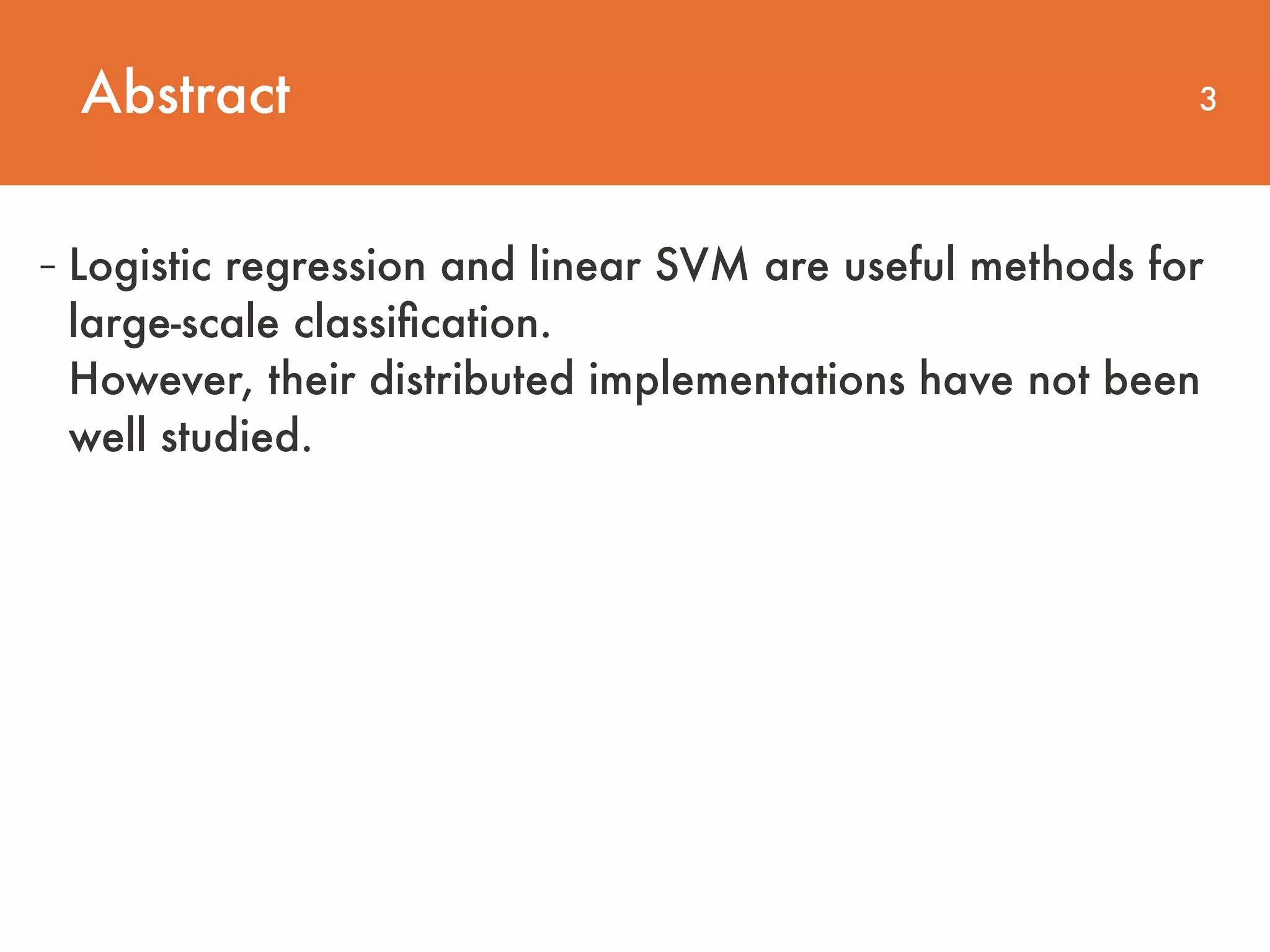
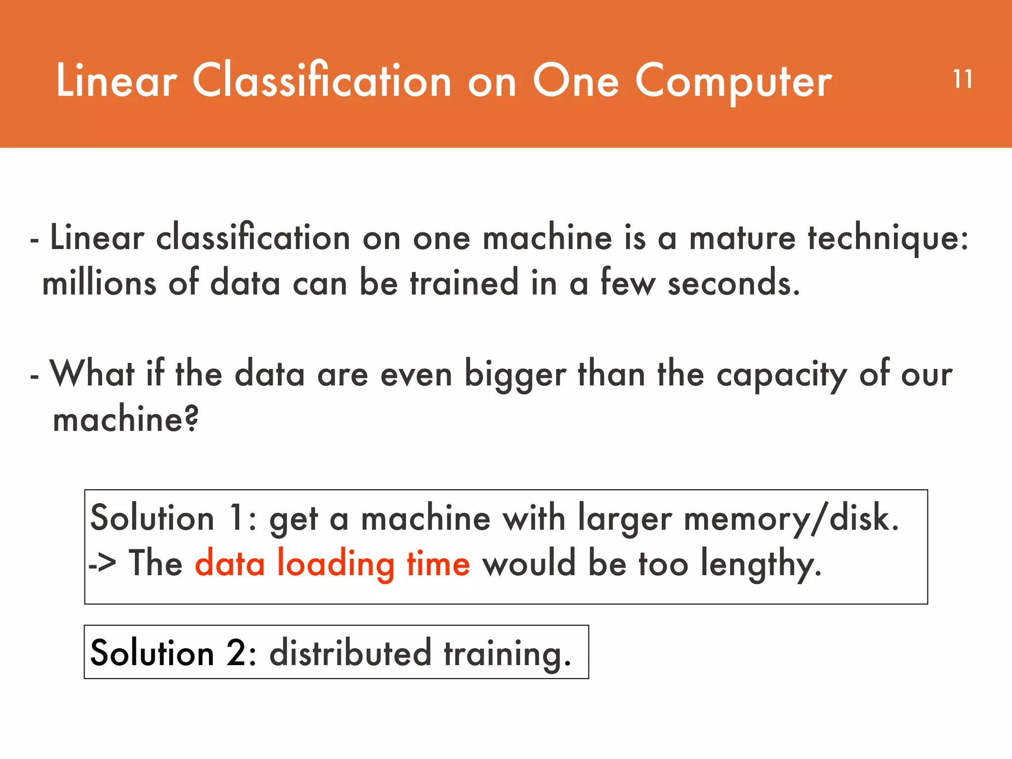
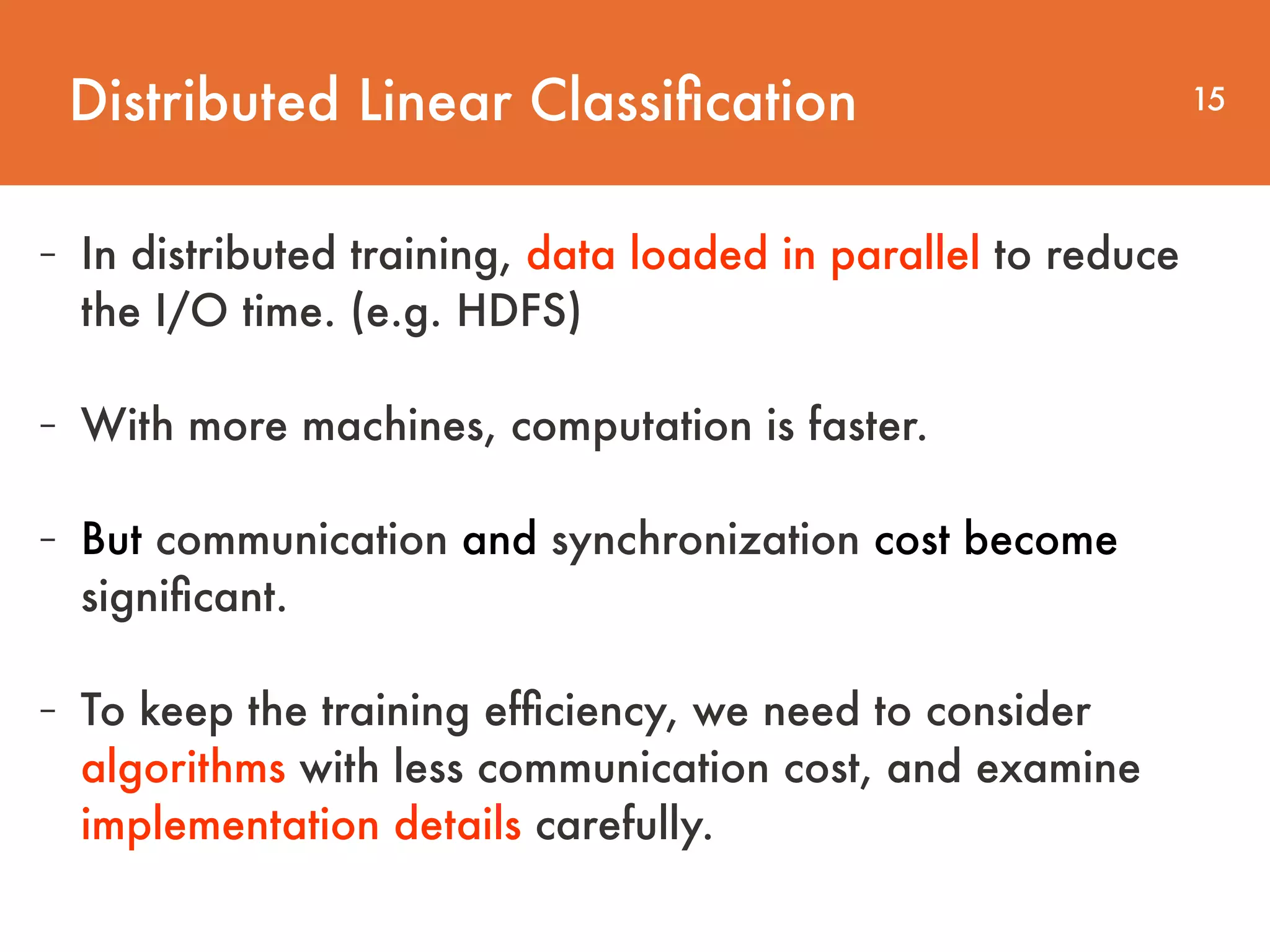
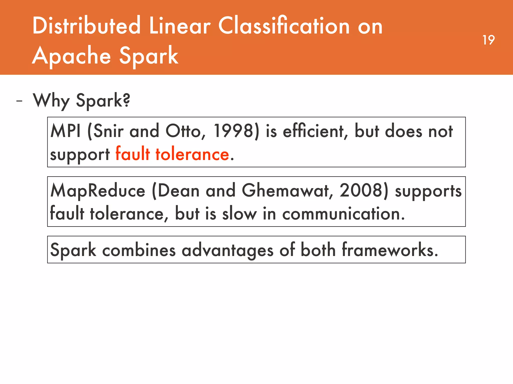
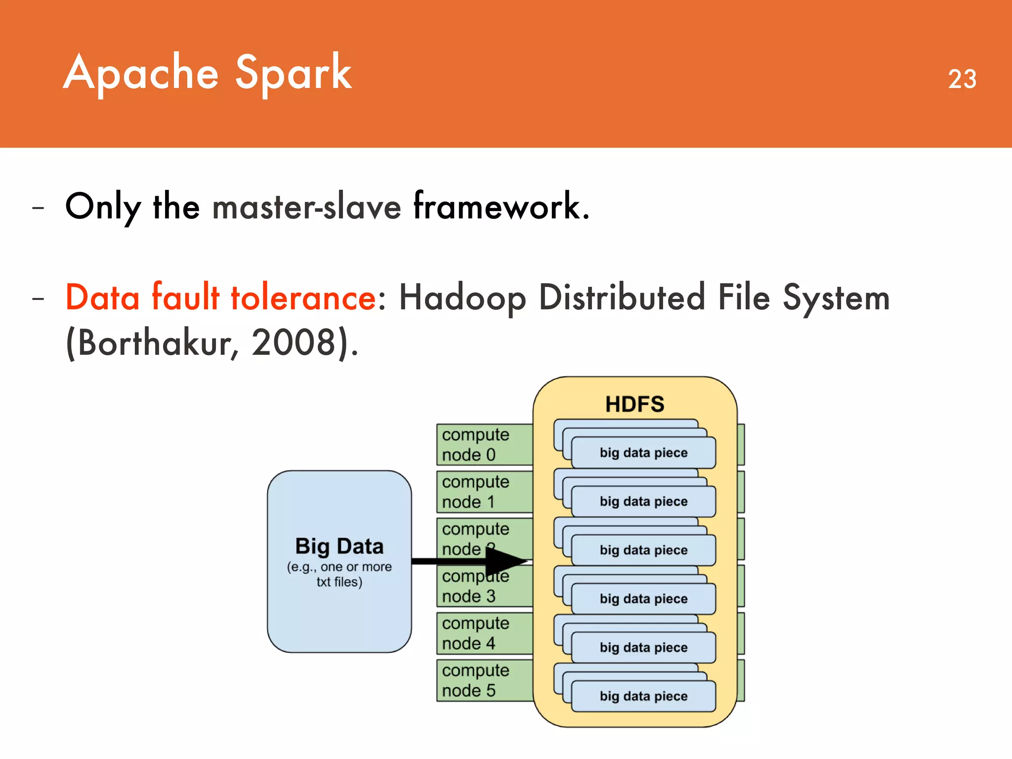
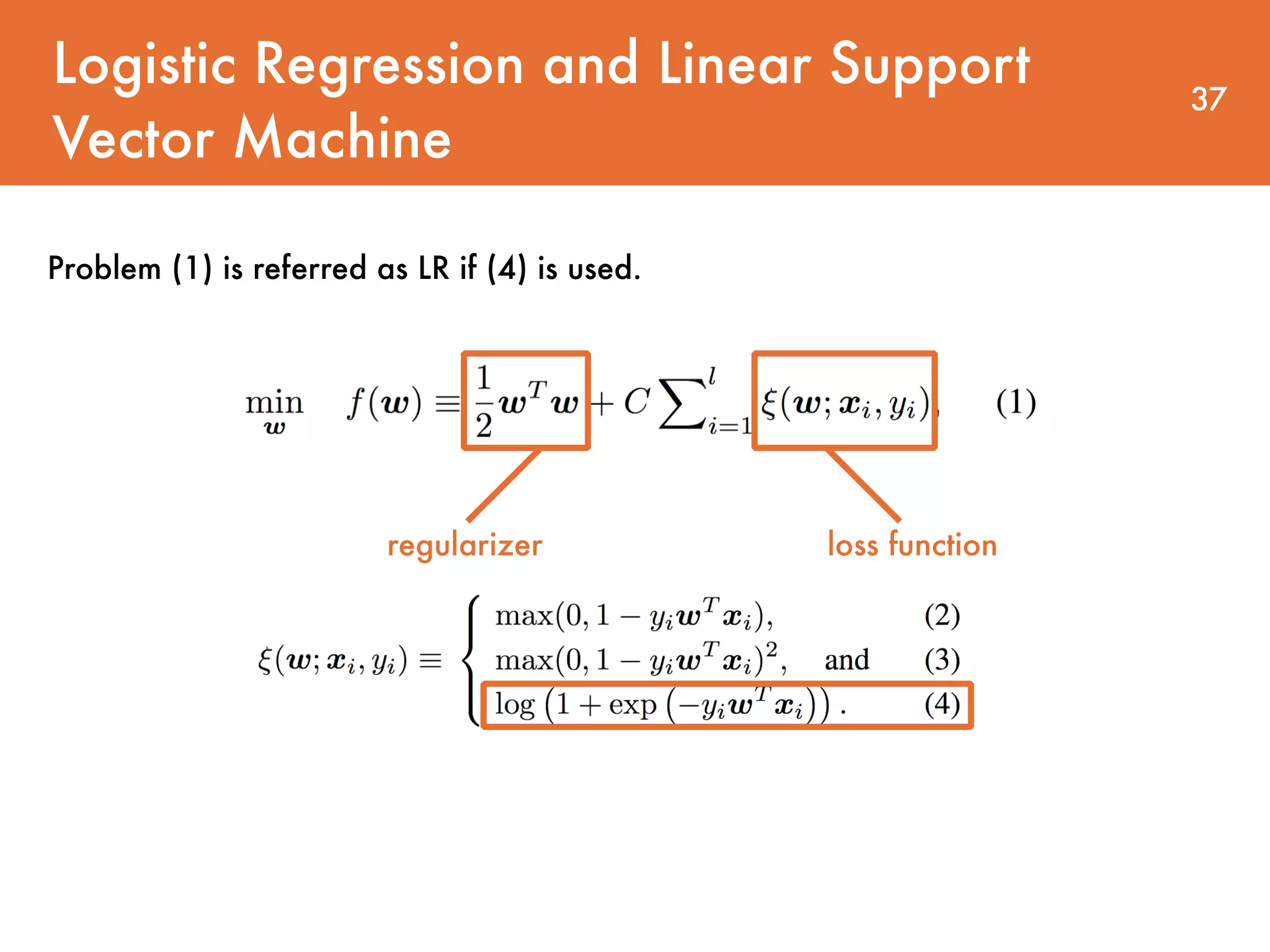
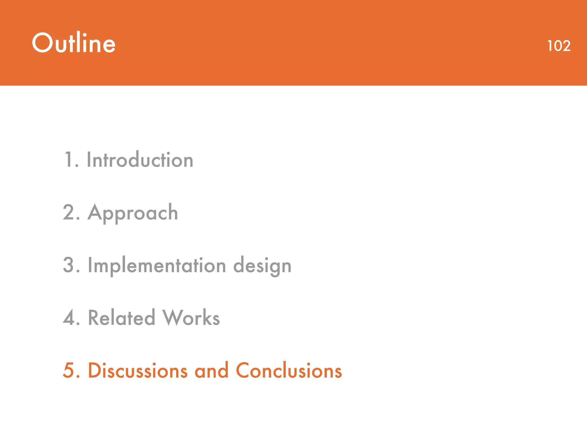
![30 package org.apache.spark.examples import java.util.Random import org.apache.spark.{SparkConf, SparkContext} import org.apache.spark.SparkContext._ /** * Usage: GroupByTest [numMappers] [numKVPairs] [valSize] [numReducers] */ object GroupByTest { def main(args: Array[String]) { val sparkConf = new SparkConf().setAppName("GroupBy Test") var numMappers = 100 var numKVPairs = 10000 var valSize = 1000 var numReducers = 36 val sc = new SparkContext(sparkConf) val pairs1 = sc.parallelize(0 until numMappers, numMappers).flatMap { p => val ranGen = new Random var arr1 = new Array[(Int, Array[Byte])] (numKVPairs) for (i <- 0 until numKVPairs) { val byteArr = new Array[Byte](valSize) ranGen.nextBytes(byteArr) arr1(i) = (ranGen.nextInt(Int.MaxValue), byteArr) } arr1 }.cache // Enforce that everything has been calculated and in cache pairs1.count println(pairs1.groupByKey(numReducers).count) sc.stop() } } GroupByTest.scala [1]. Initialize SparkConf. [2]. Initialize numMappers=100, numKVPairs=10,000, valSize=1000, numReducers= 36. [3]. Initialize SparkContext, which creates the necessary objects and actors for the driver. [4].Each mapper creats an arr1: Array[(Int, Byte[])], which has numKVPairs elements. Each Int is a random integer, and each byte array's size is valSize. We can estimate Size(arr1) = numKVPairs * (4 + valSize) = 10MB, so that Size(pairs1) = numMappers * Size(arr1) =1000MB. [5].Each mapper is instructed to cache its arr1 array into the memory. [6].The action count() is applied to sum the number of elements in arr1 in all mappers, the result is numMappers * numKVPairs = 1,000,000. This action triggers the caching of arr1s. [7].groupByKey operation is performed on cached pairs1. The reducer number (a.k.a., partition number) is numReducers. Theoretically, if hash(key) is evenly distributed, each reducer will receive numMappers * numKVPairs / numReducer = 27,777 pairs of (Int, Array[Byte]), with a size of Size(pairs1) / numReducer = 27MB. [8].Reducer aggregates the records with the same Int key, the result is (Int, List(Byte[], Byte[], ..., Byte[])). [9].Finally, a count() action sums up the record number in each reducer, the final result is actually the number of distinct integers in pairs1. - Lineage (Zaharia et al., 2012). spark code explanation Apache Spark (skip)](https://image.slidesharecdn.com/large-scalelogisticregressionandlinearsupportvectormachinesusingspark-161108042002/75/Large-scale-logistic-regression-and-linear-support-vector-machines-using-spark-30-2048.jpg)
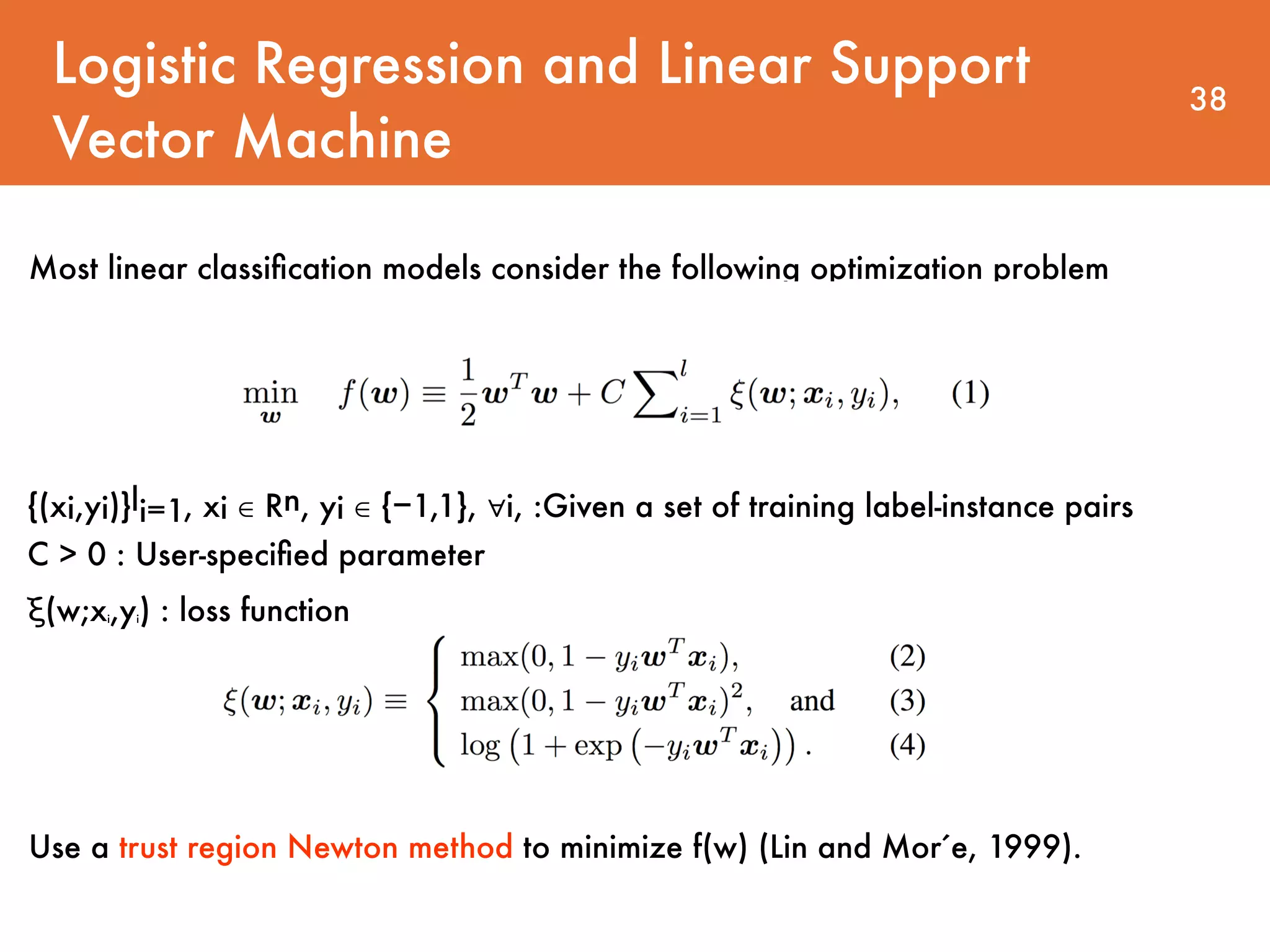


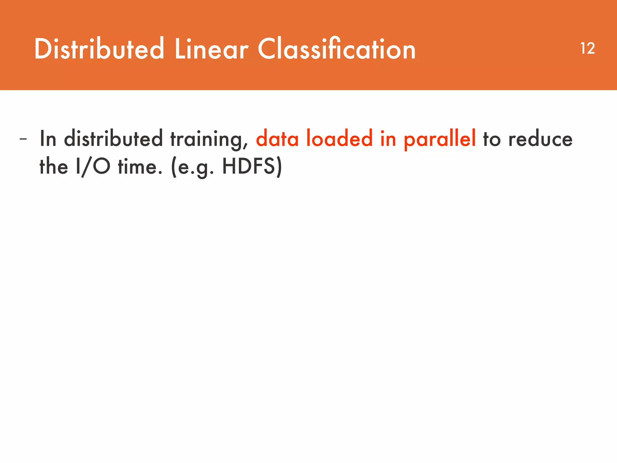
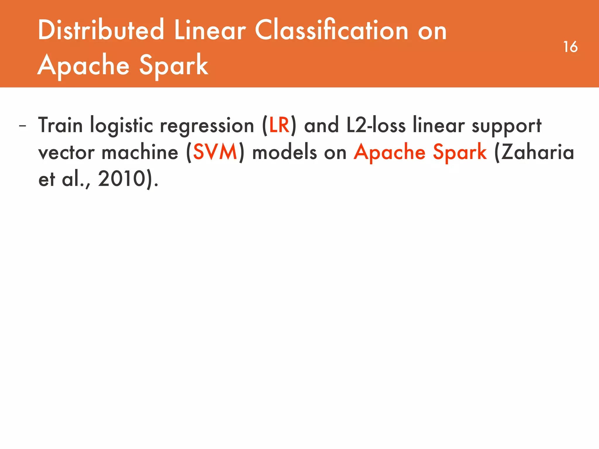
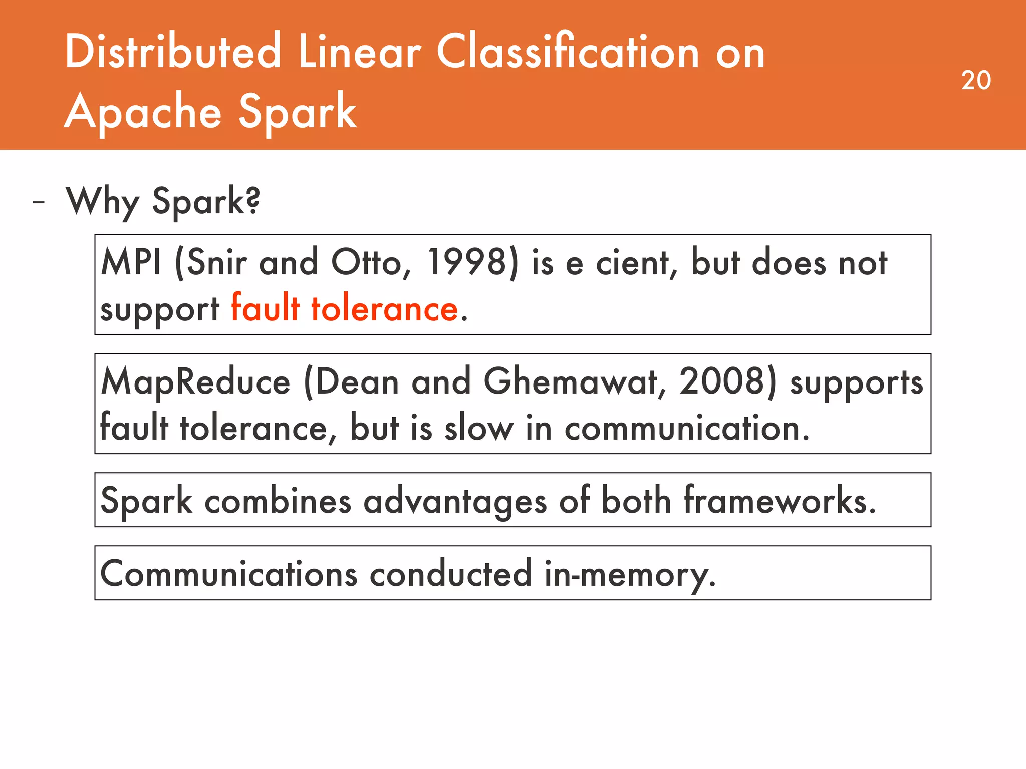
![Implementation design 53 - In this section, they study implementation issues for their
software. - They name their distributed TRON implementation Spark LIBLINEAR because algorithmically it is an extension of the TRON implementation in the software LIBLINEAR[10]](https://image.slidesharecdn.com/large-scalelogisticregressionandlinearsupportvectormachinesusingspark-161108042002/75/Large-scale-logistic-regression-and-linear-support-vector-machines-using-spark-53-2048.jpg)
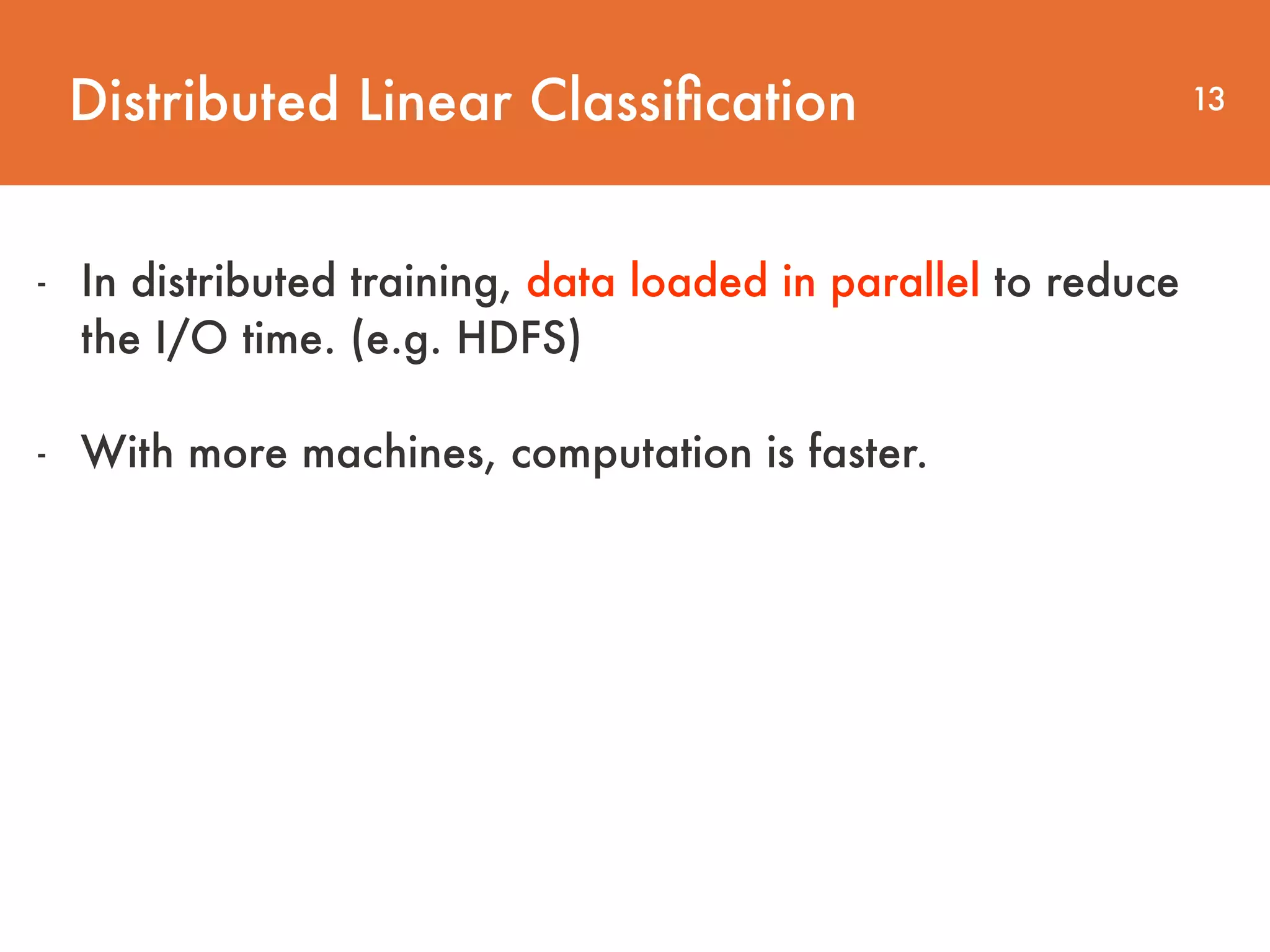
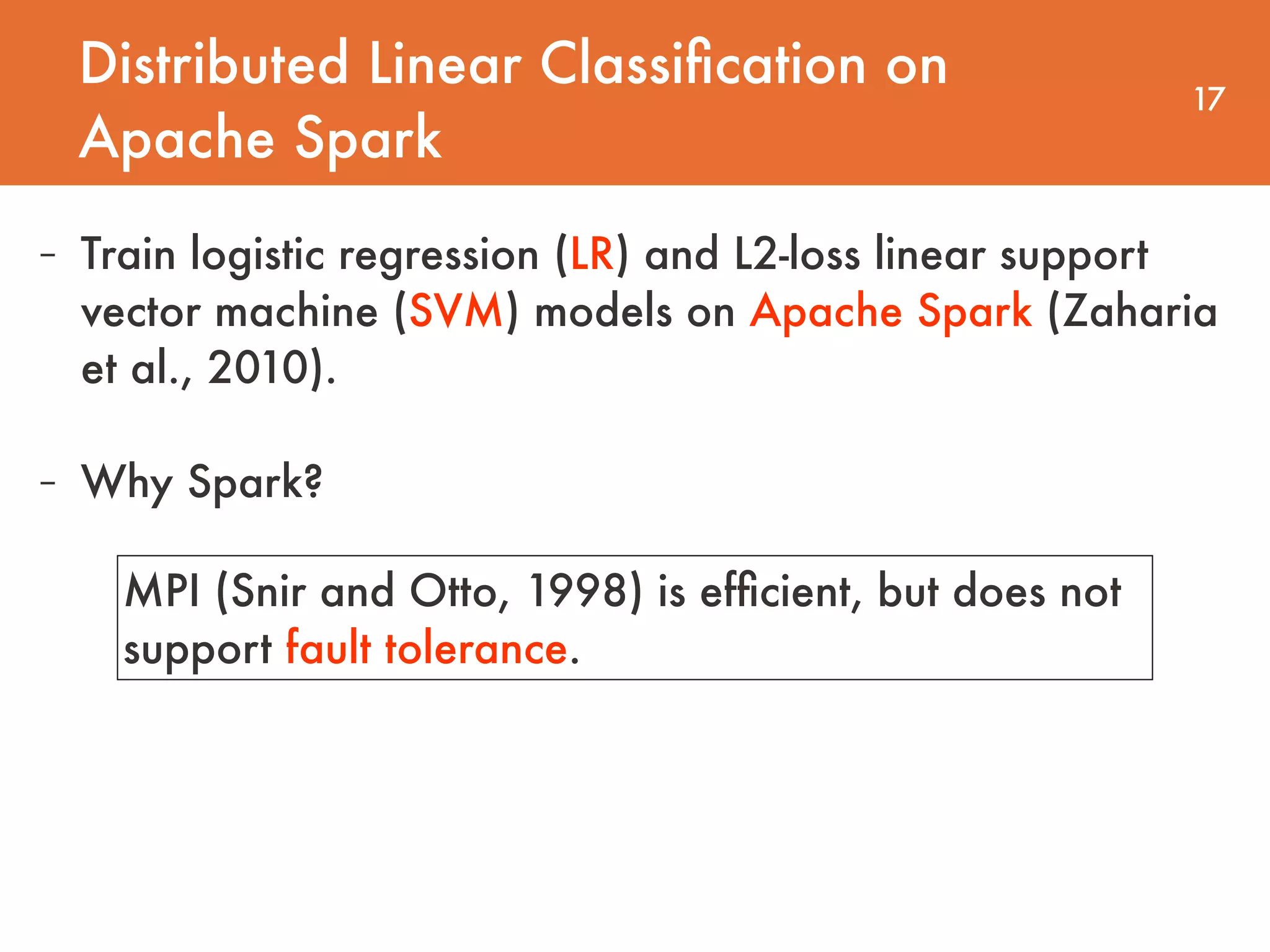
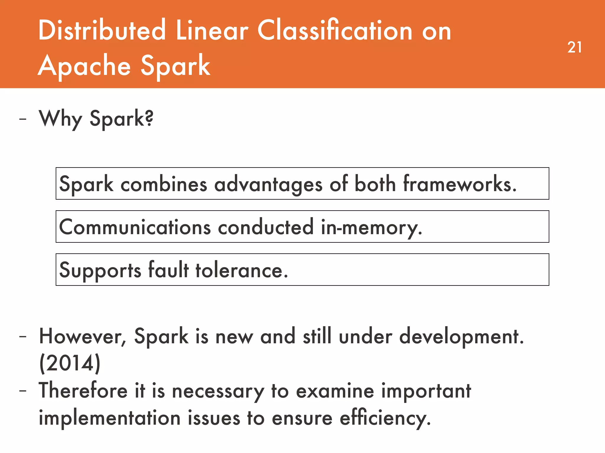
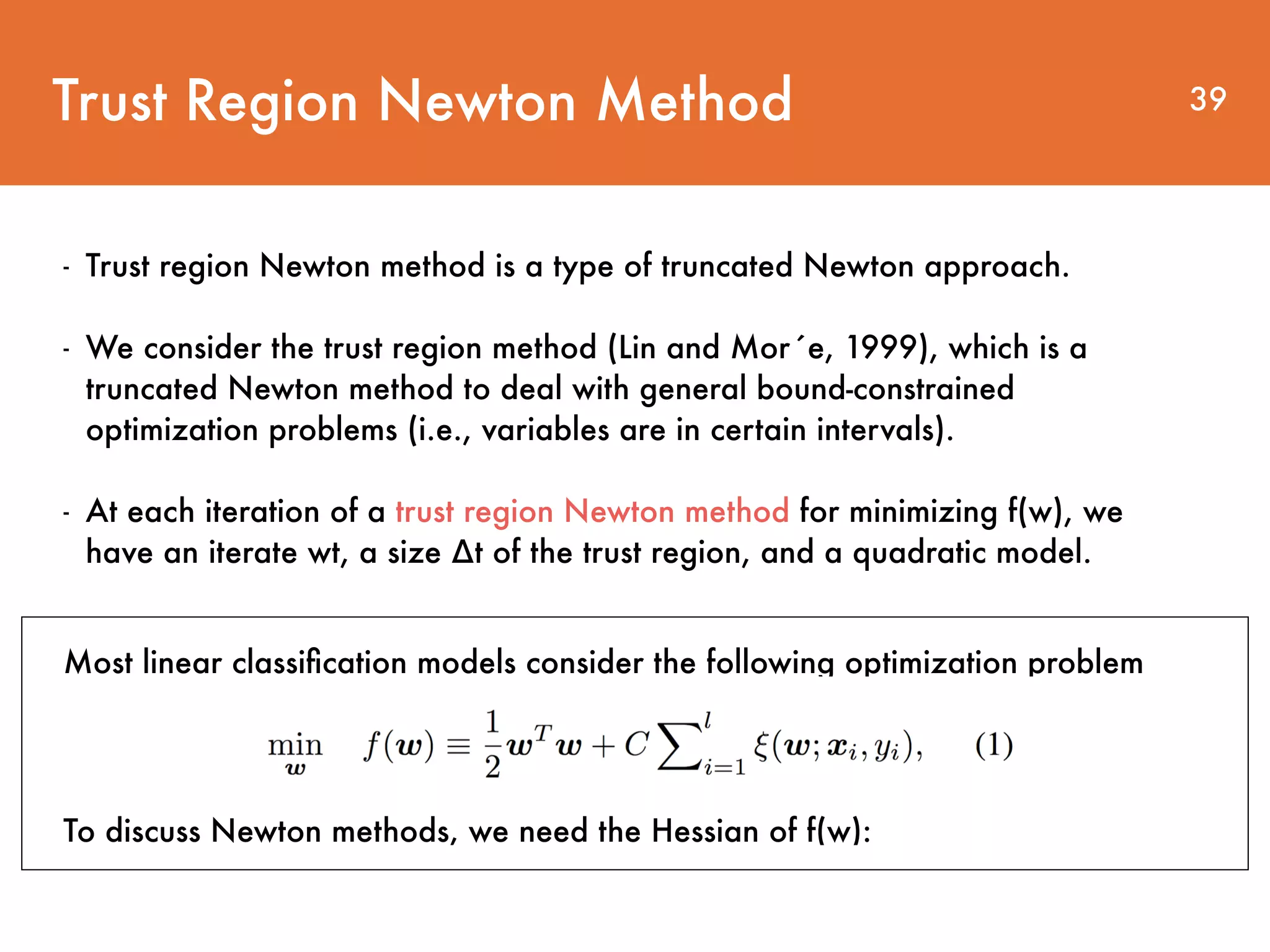
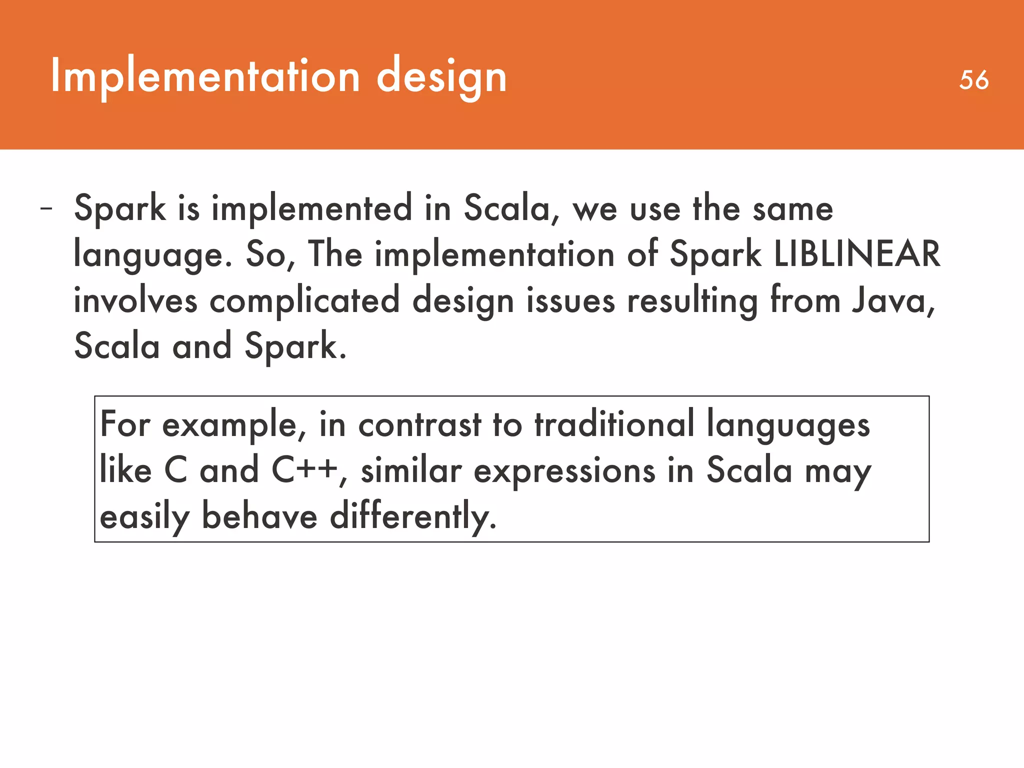
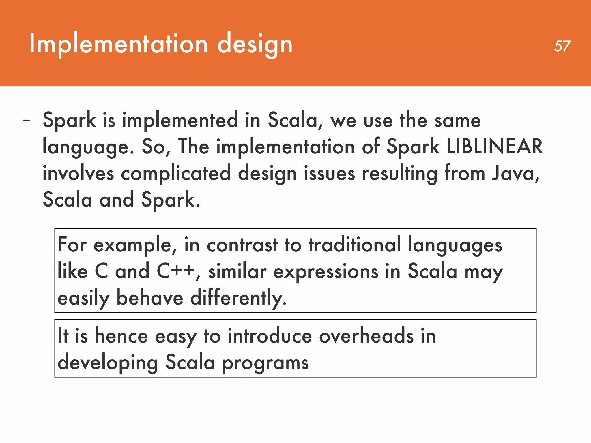
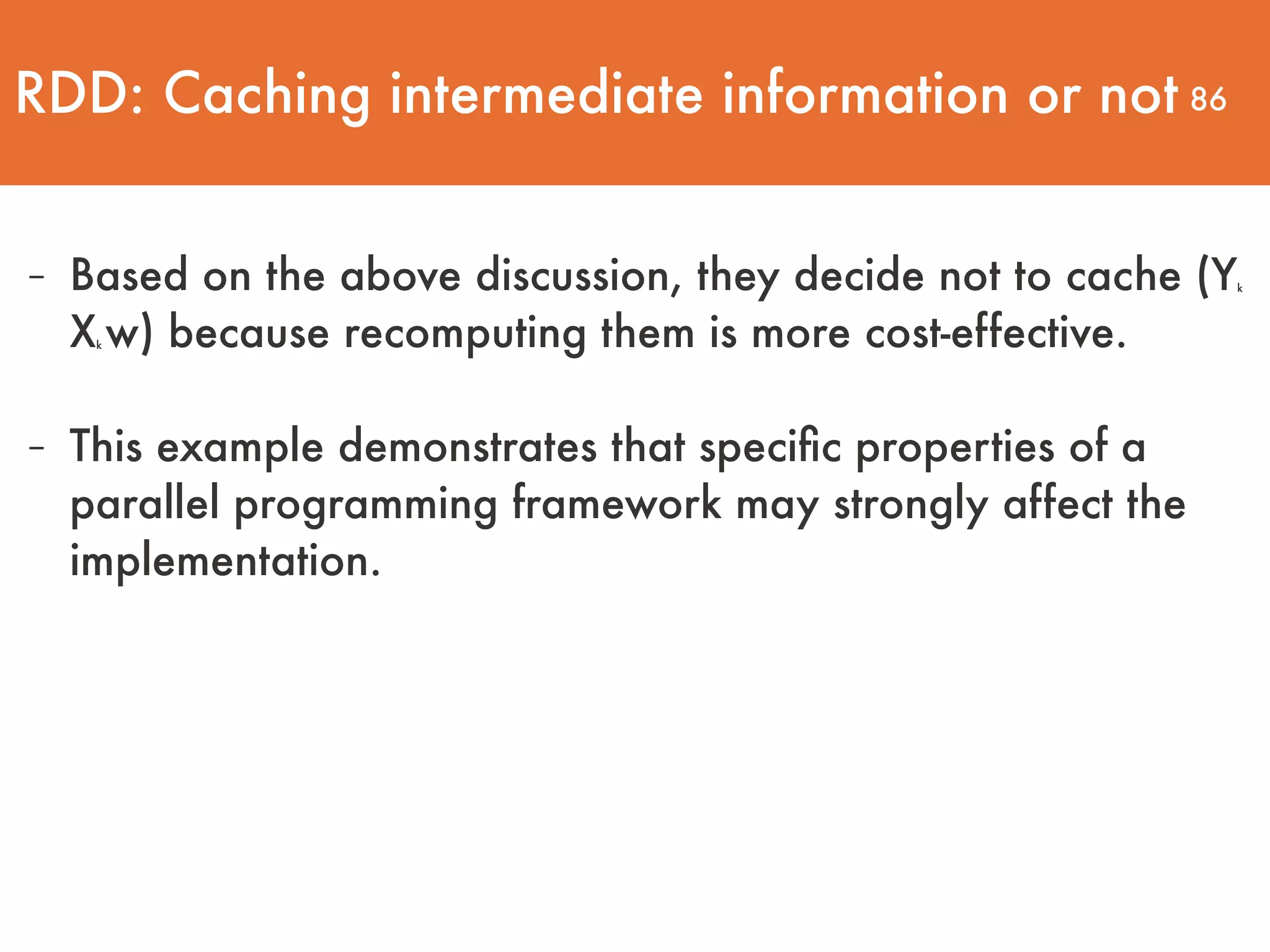
![Implementation design 54 - In this section, they study implementation issues for their
software. - They name their distributed TRON implementation Spark LIBLINEAR because algorithmically it is an extension of the TRON implementation in the software LIBLINEAR[10] - Spark is implemented in Scala, we use the same language. So, The implementation of Spark LIBLINEAR involves complicated design issues resulting from Java, Scala and Spark.](https://image.slidesharecdn.com/large-scalelogisticregressionandlinearsupportvectormachinesusingspark-161108042002/75/Large-scale-logistic-regression-and-linear-support-vector-machines-using-spark-54-2048.jpg)
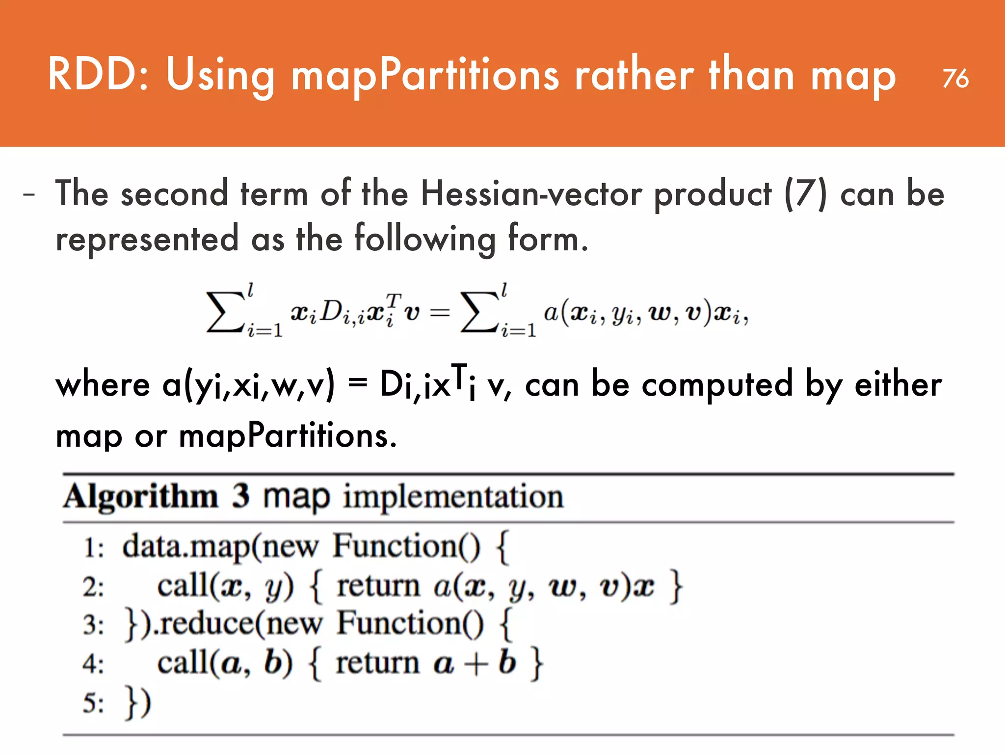
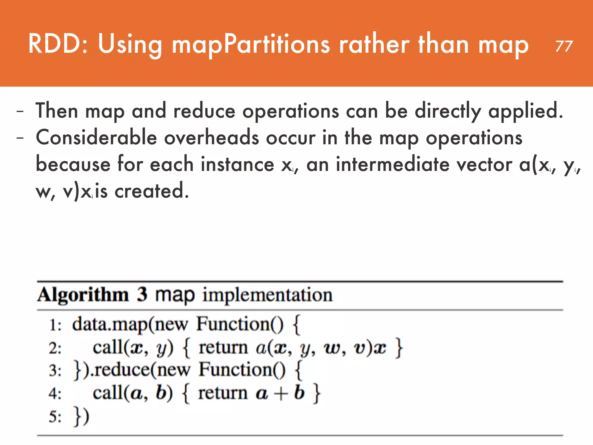
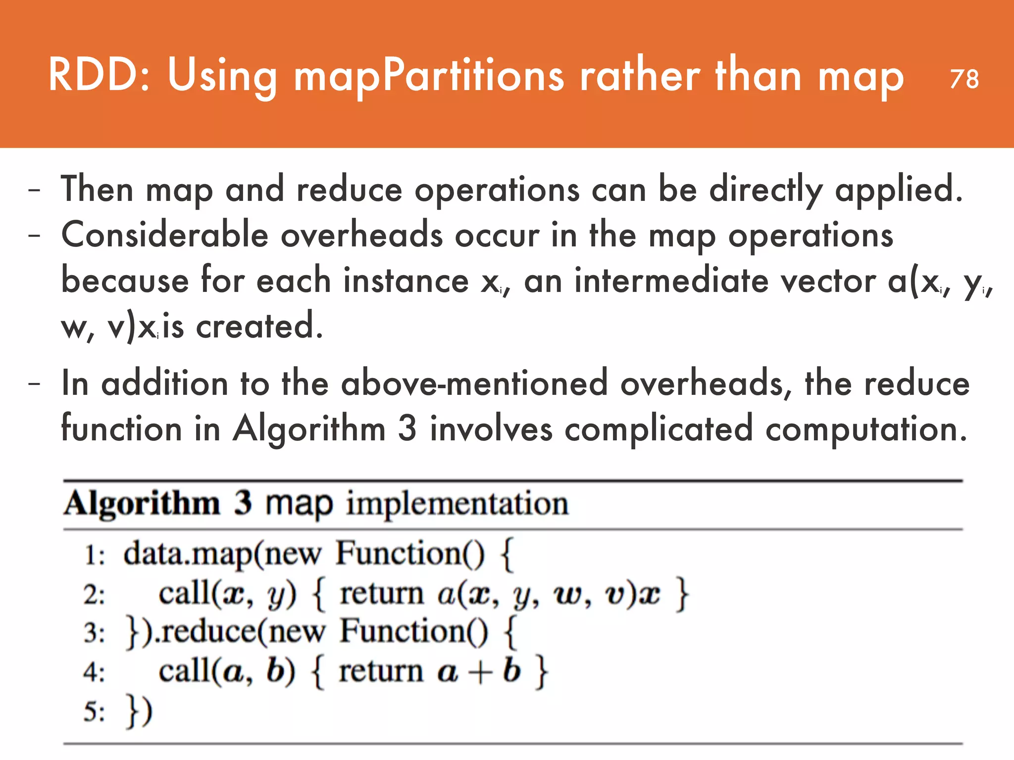
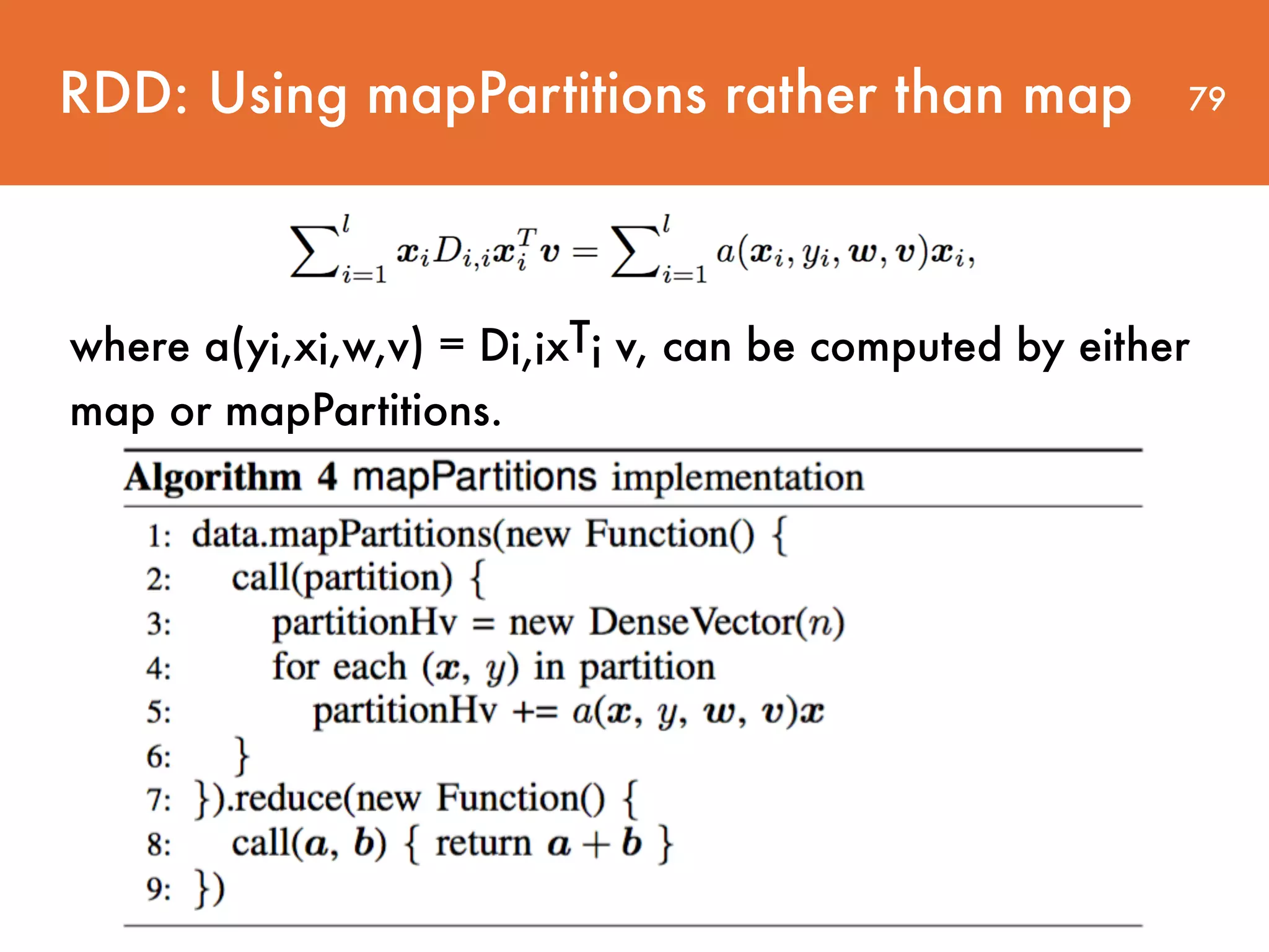

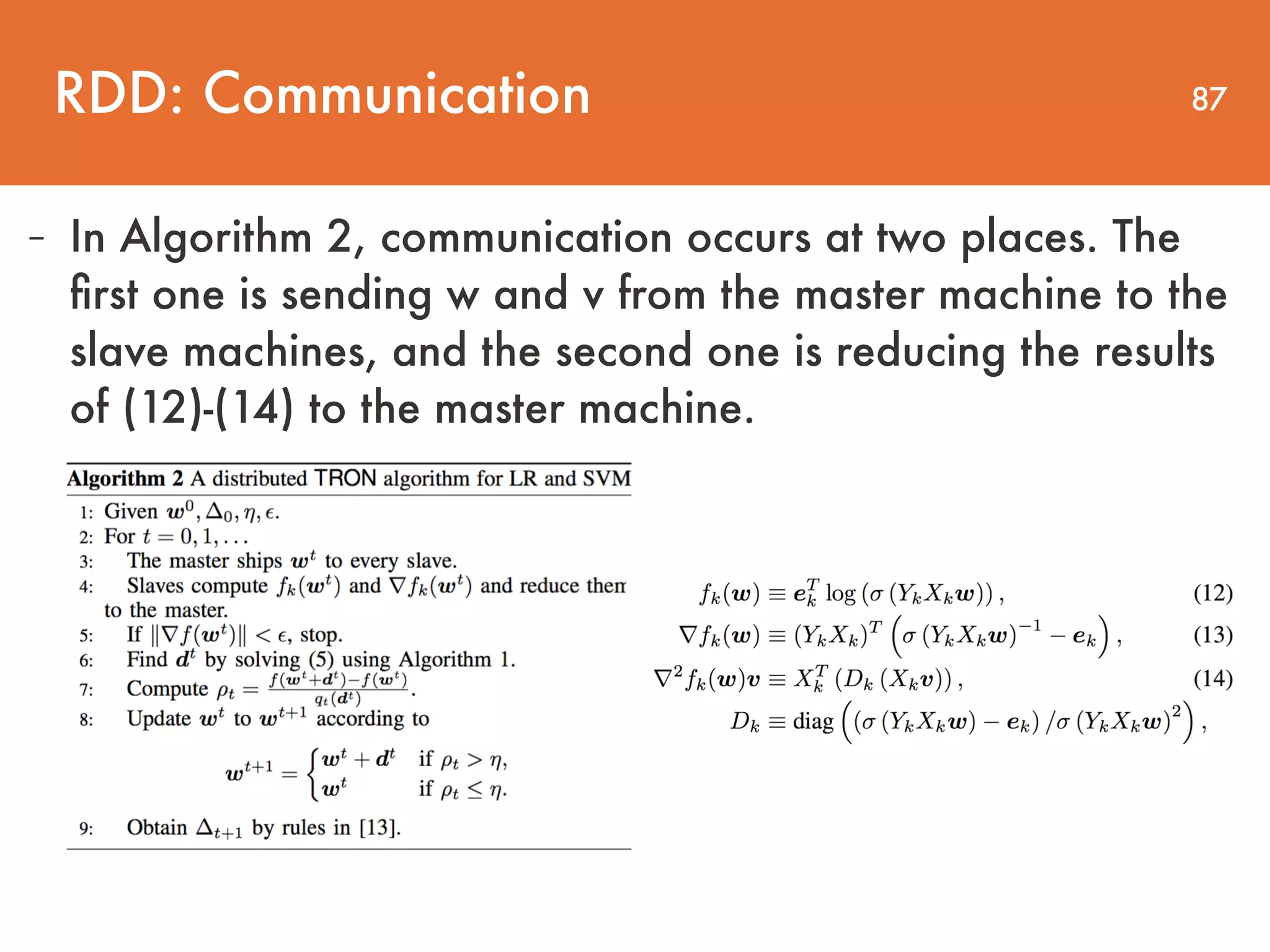


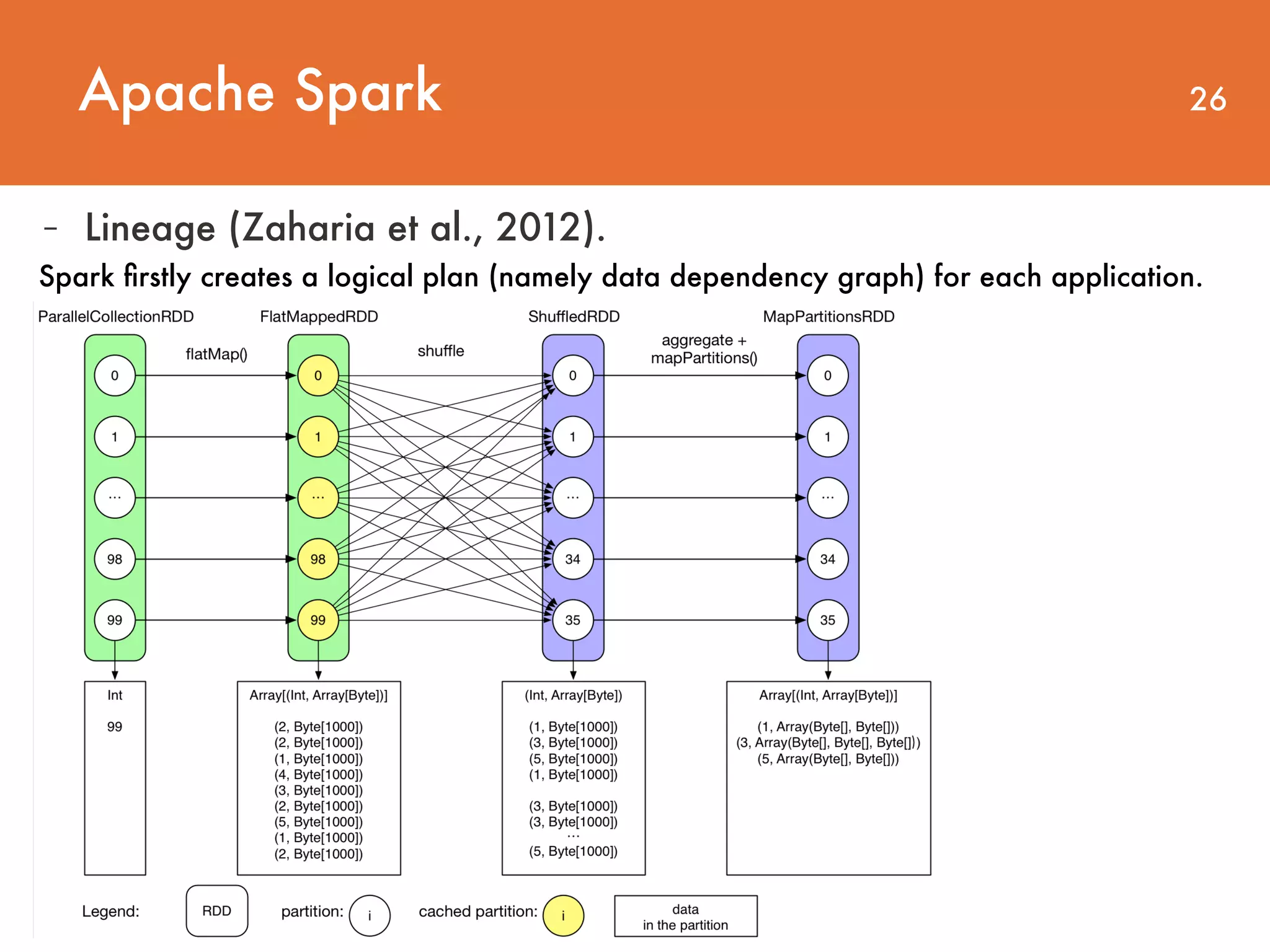
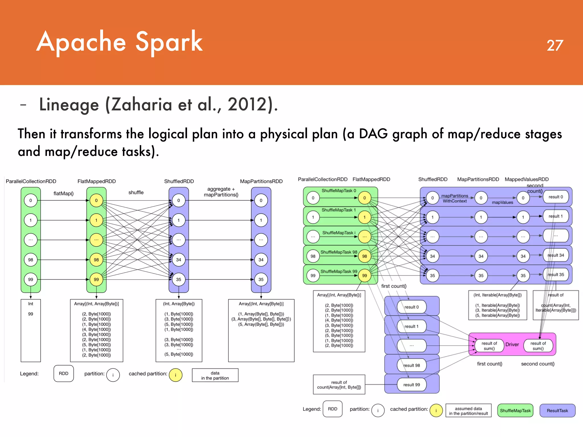
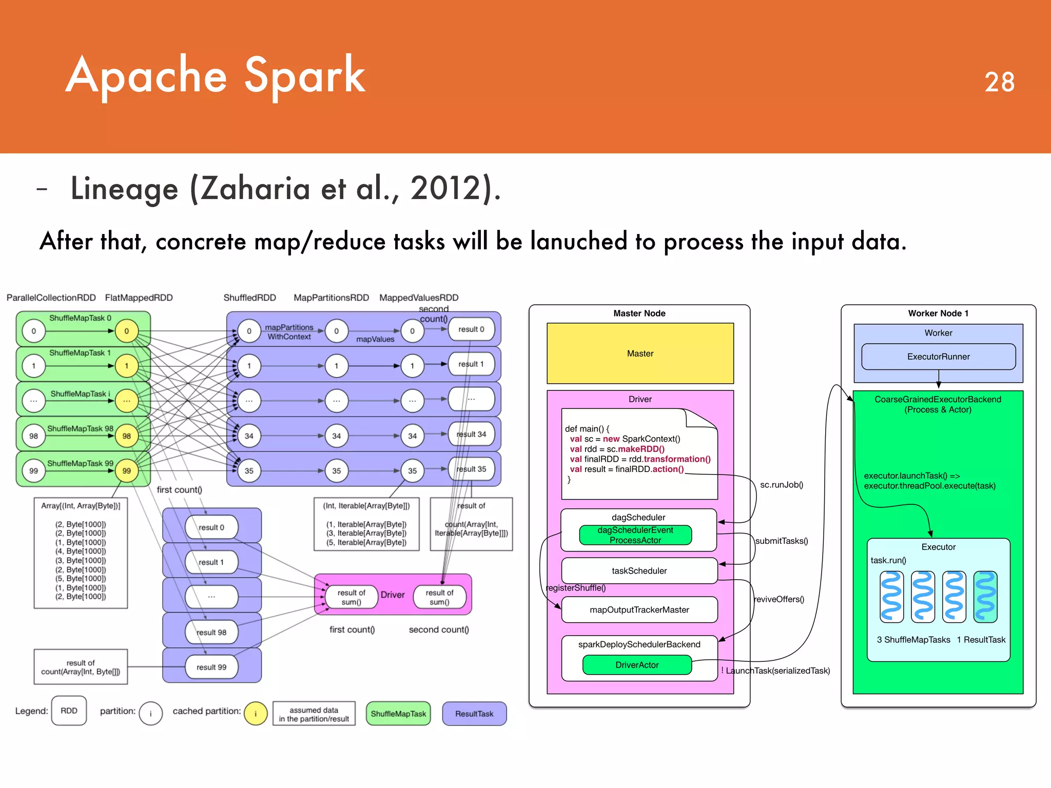
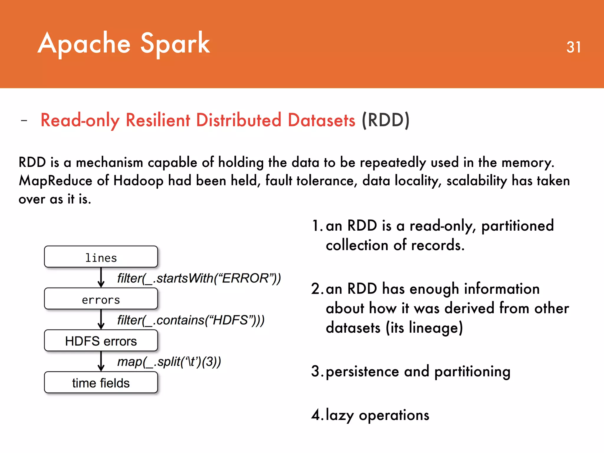
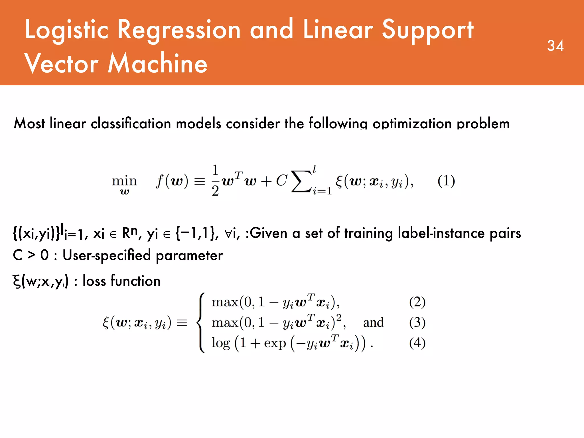
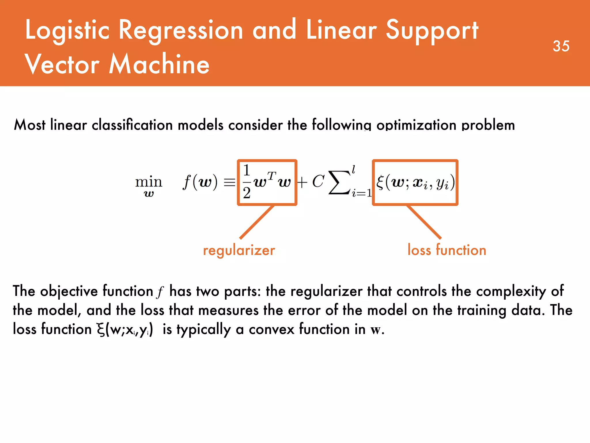
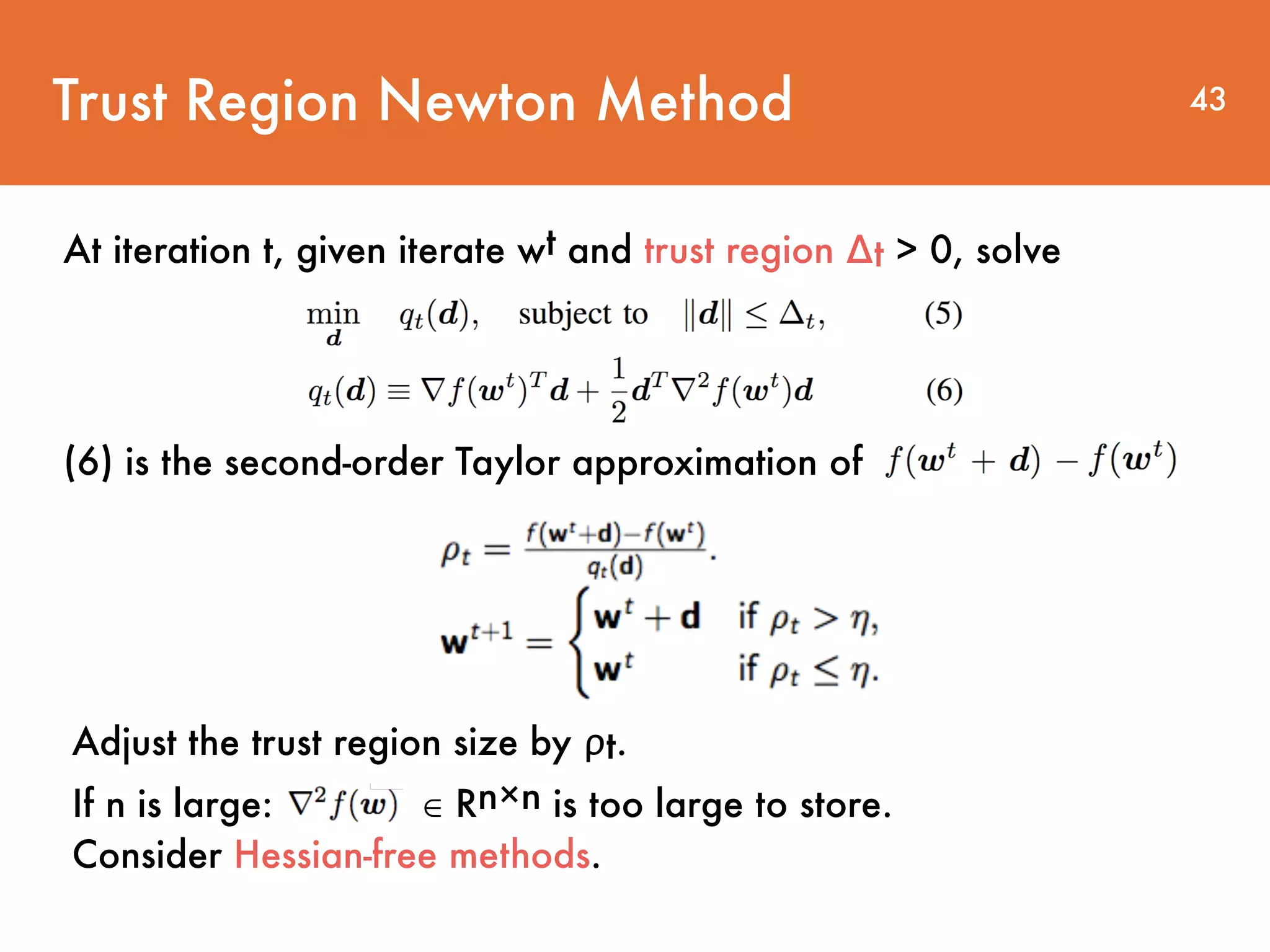
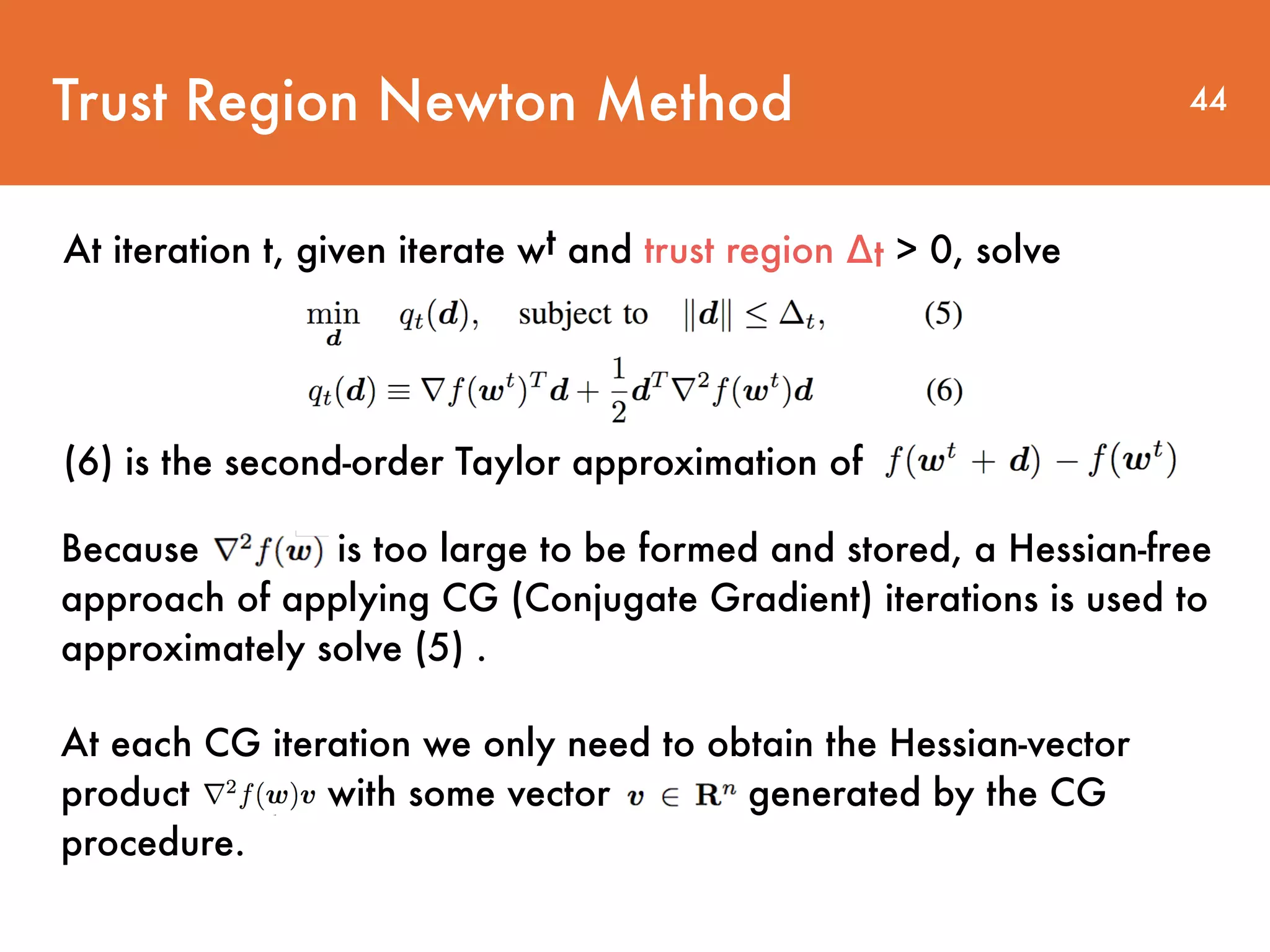
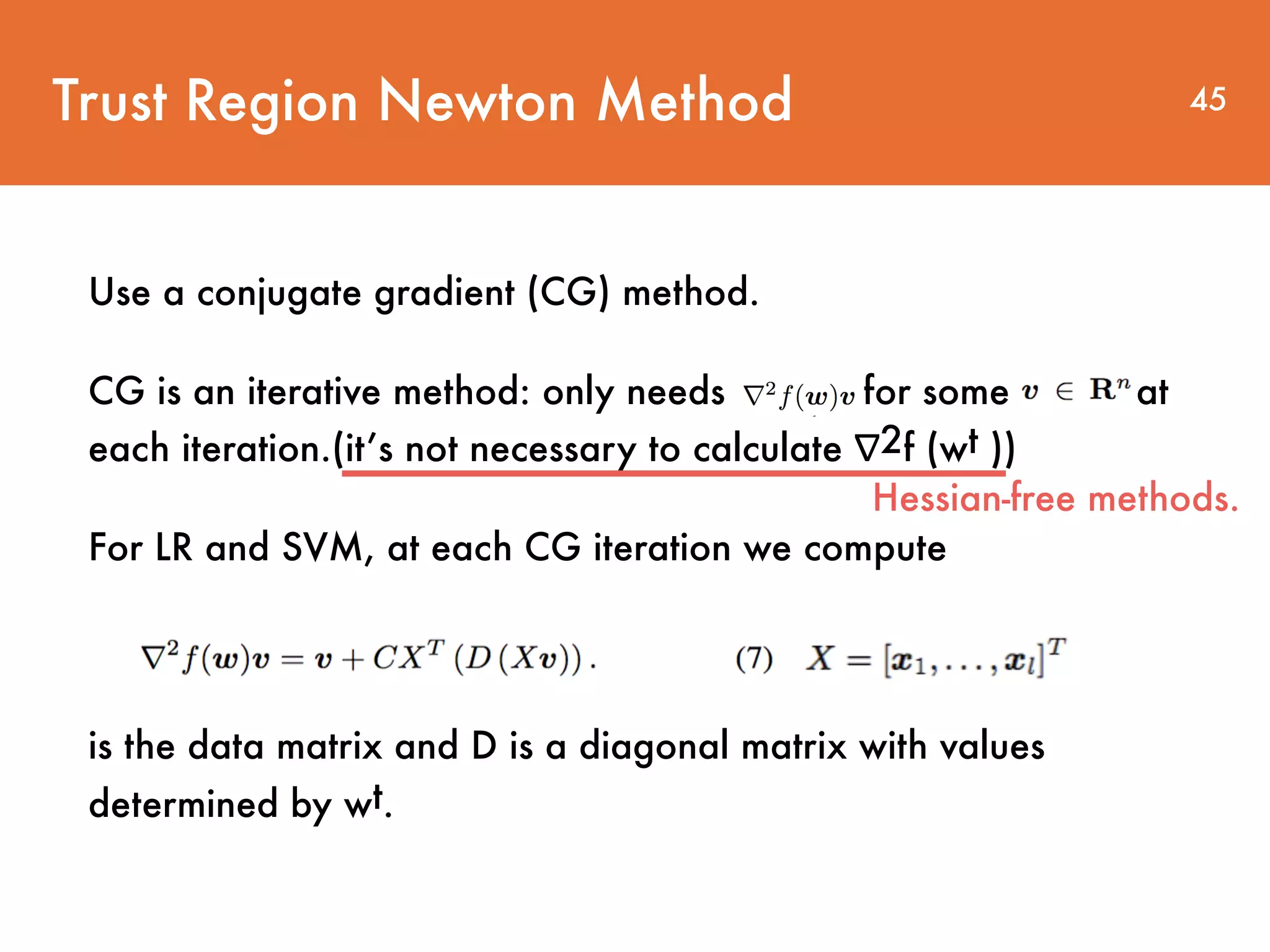
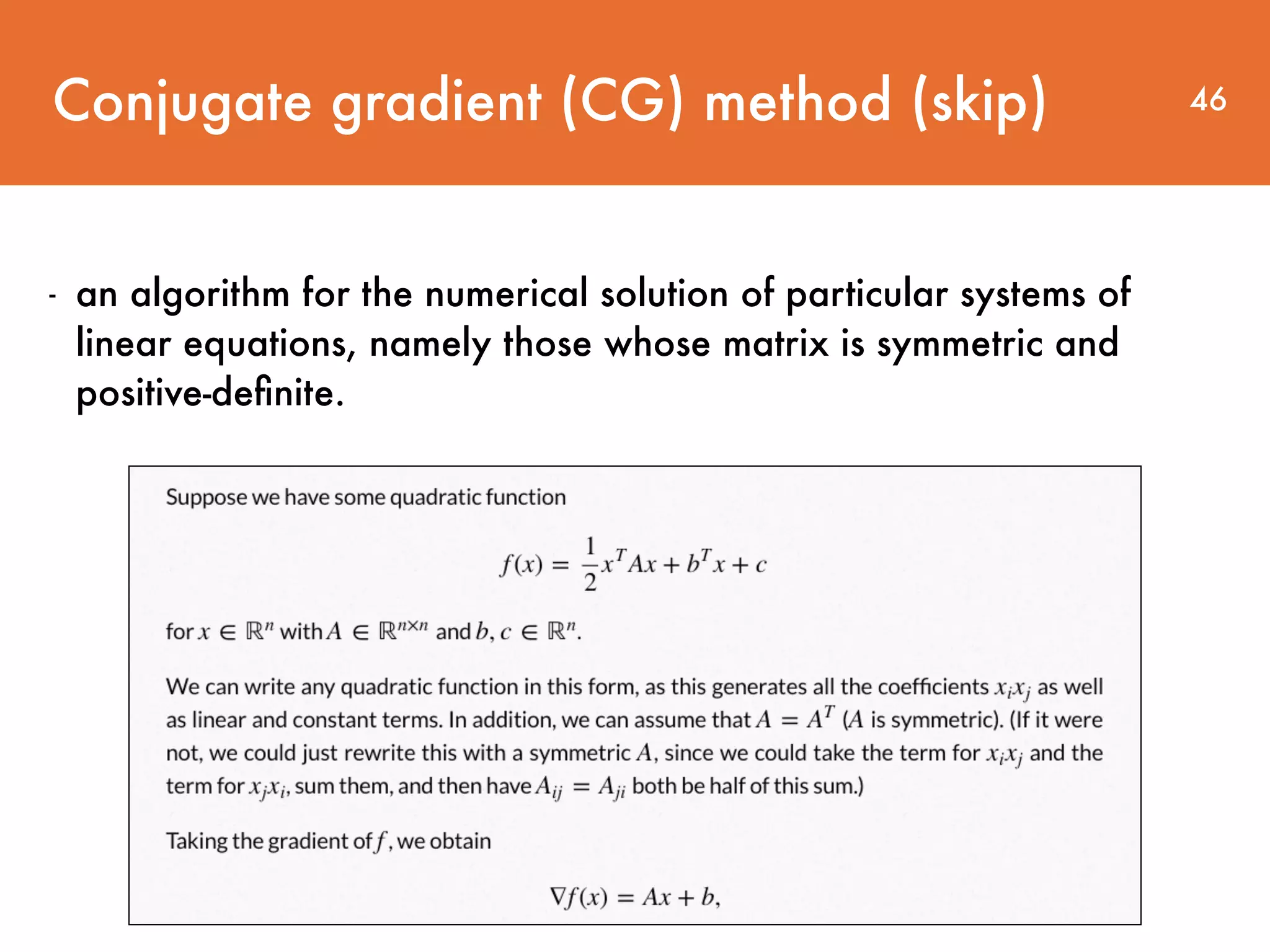
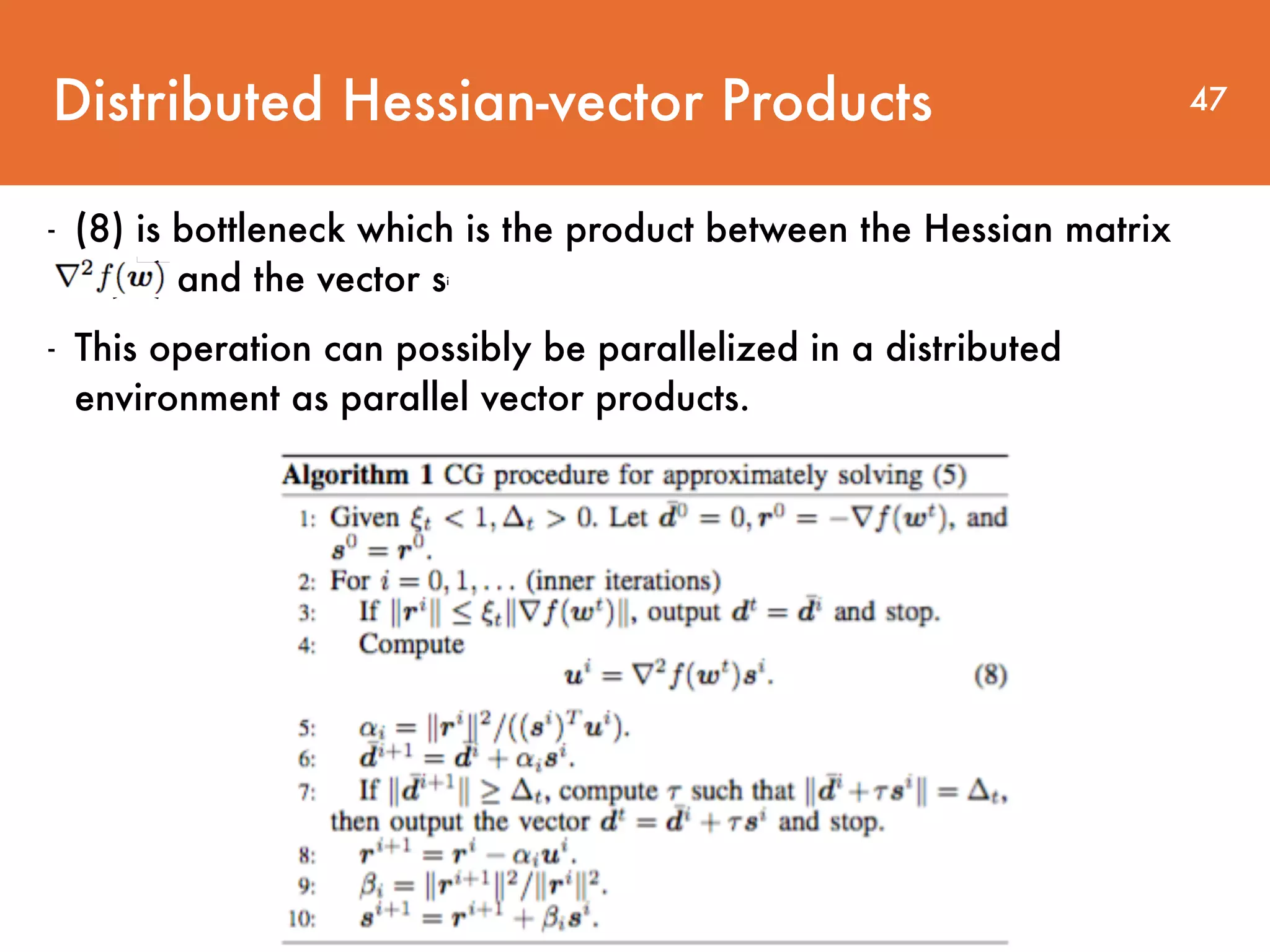
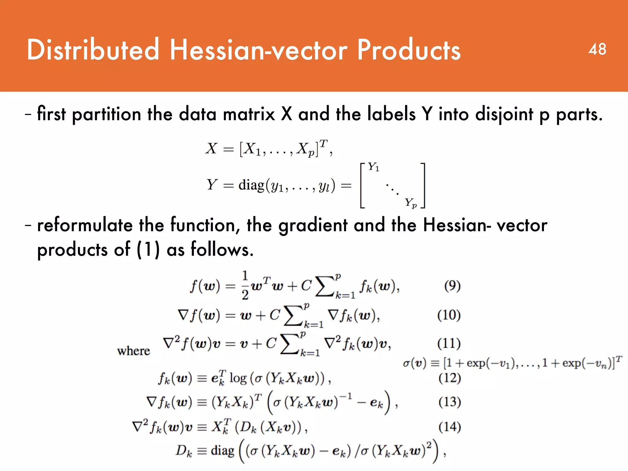
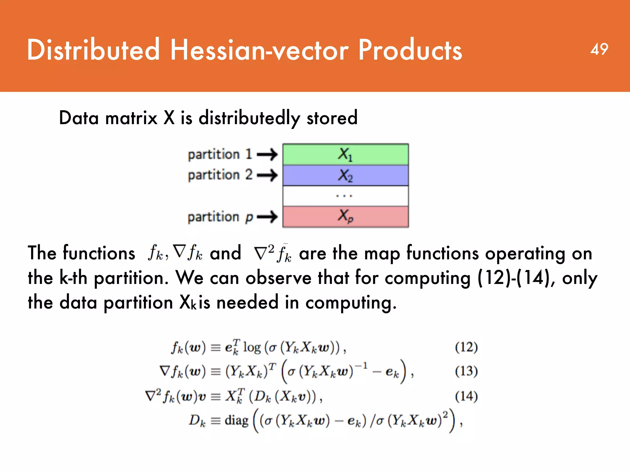
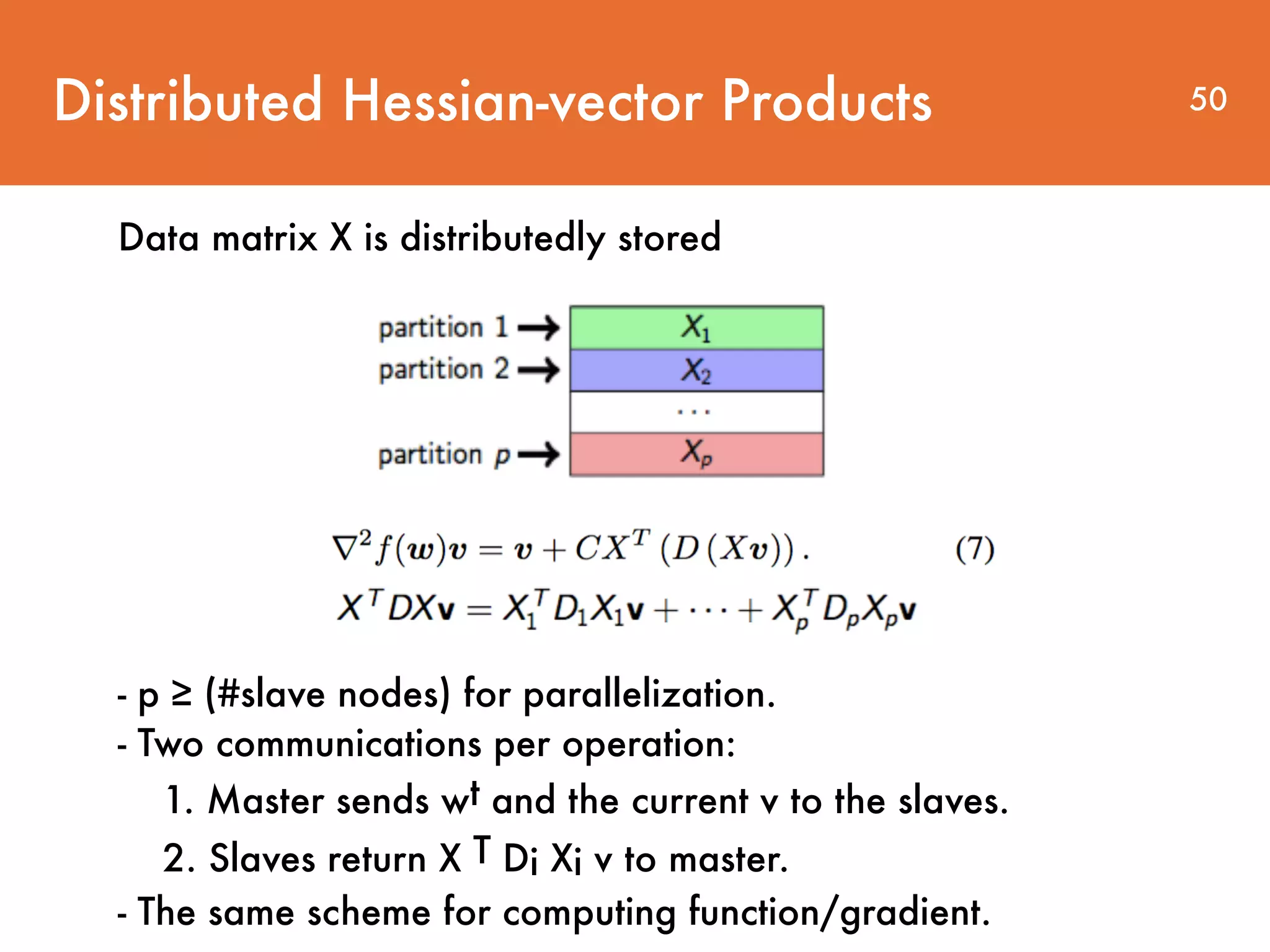
The document discusses distributed linear classification on Apache Spark. It describes using Spark to train logistic regression and linear support vector machine models on large datasets. Spark improves on MapReduce by conducting communications in-memory and supporting fault tolerance. The paper proposes using a trust region Newton method to optimize the objective functions for logistic regression and linear SVM. Conjugate gradient is used to approximate the Hessian matrix and solve the Newton system without explicitly storing the large Hessian.