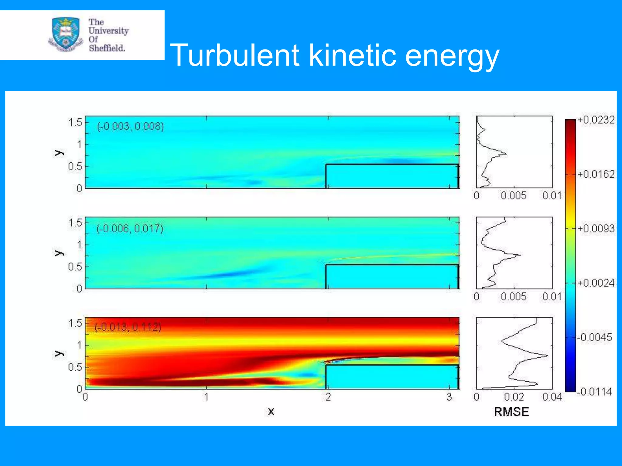
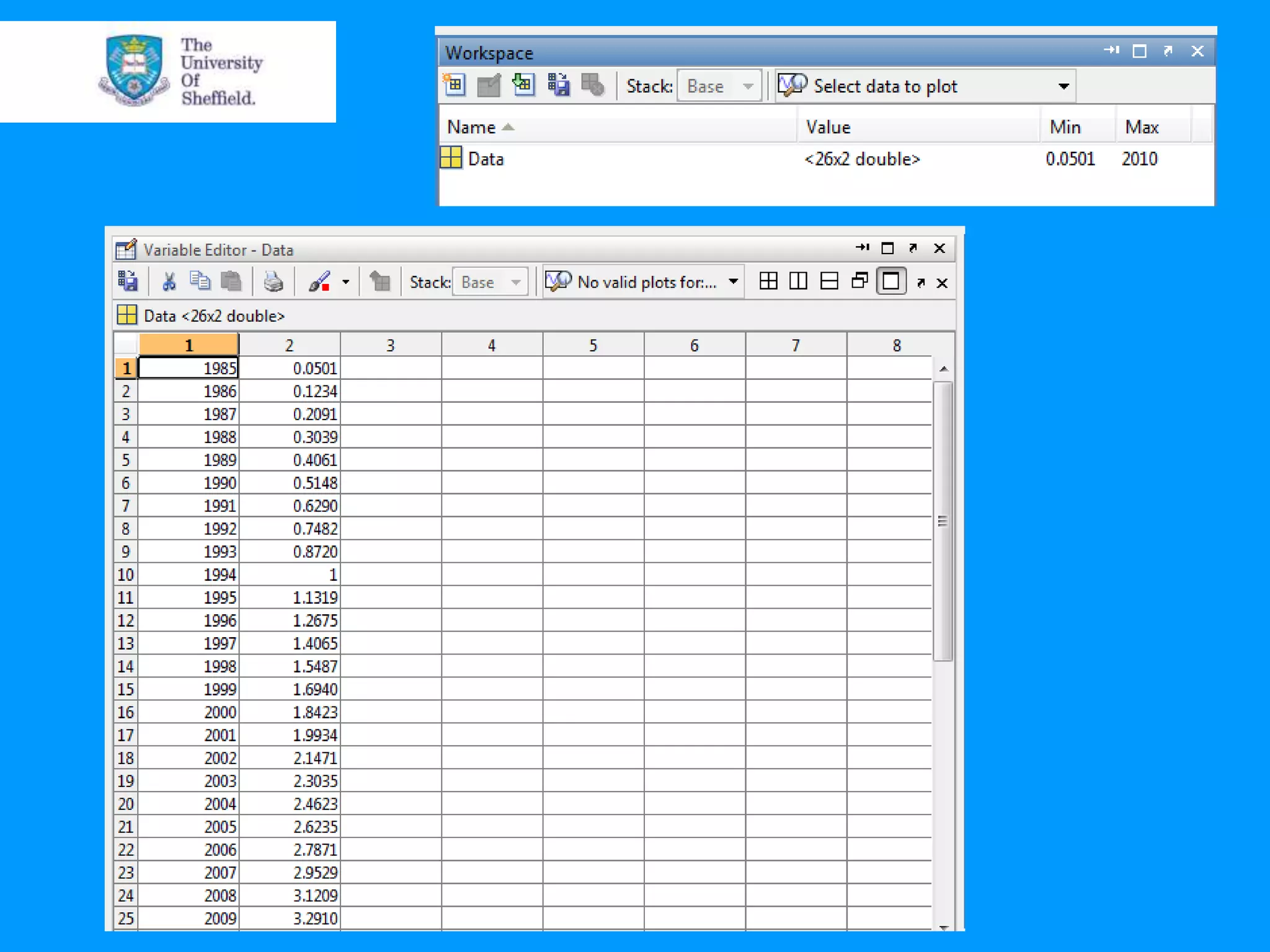
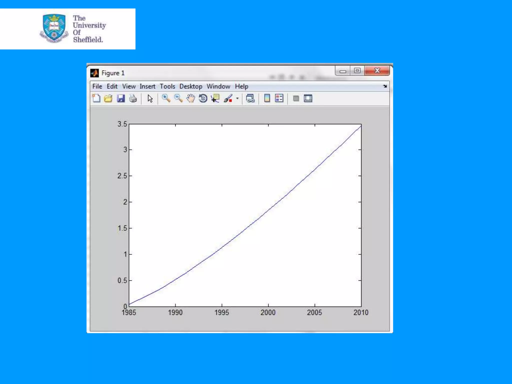
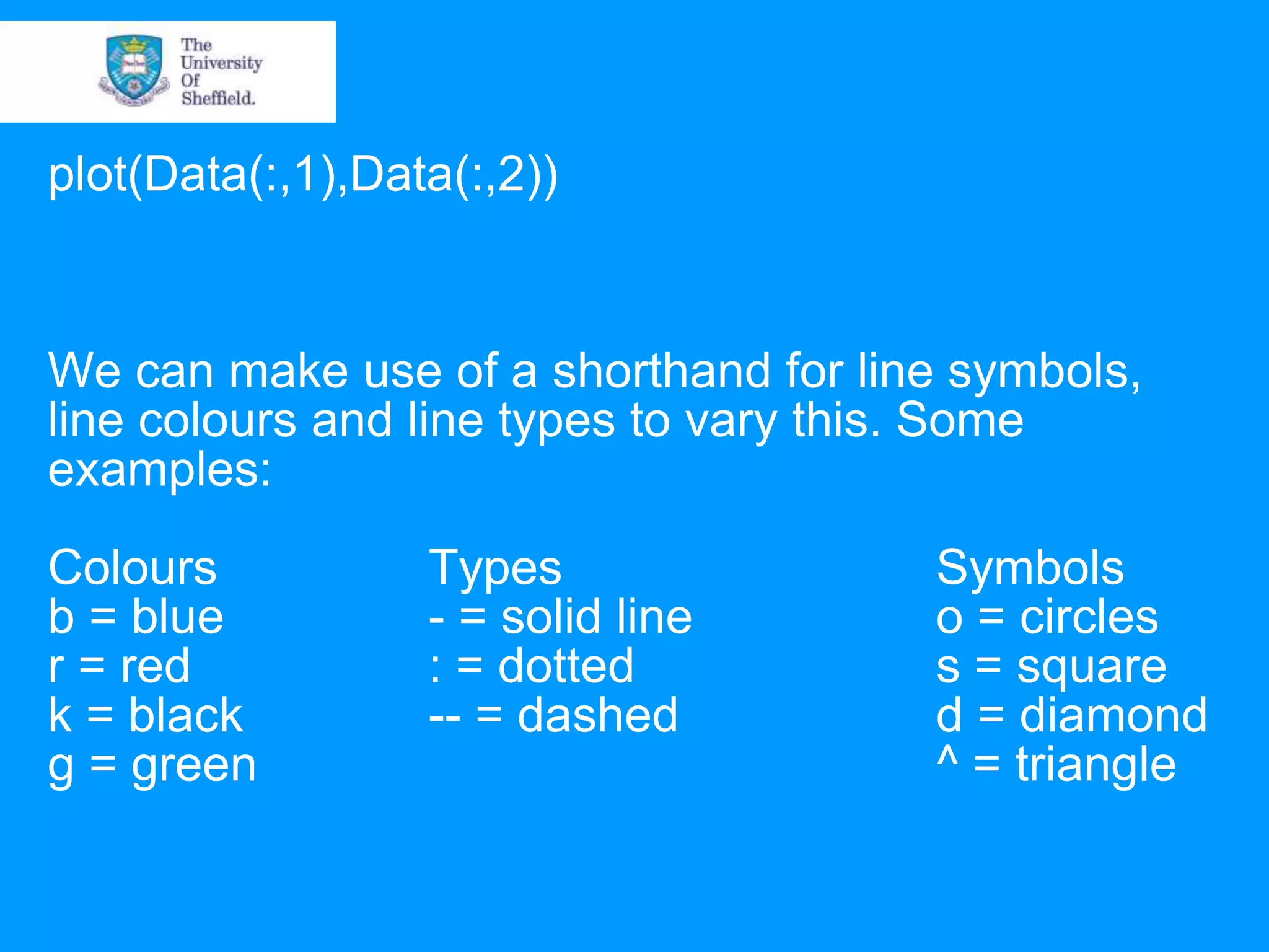
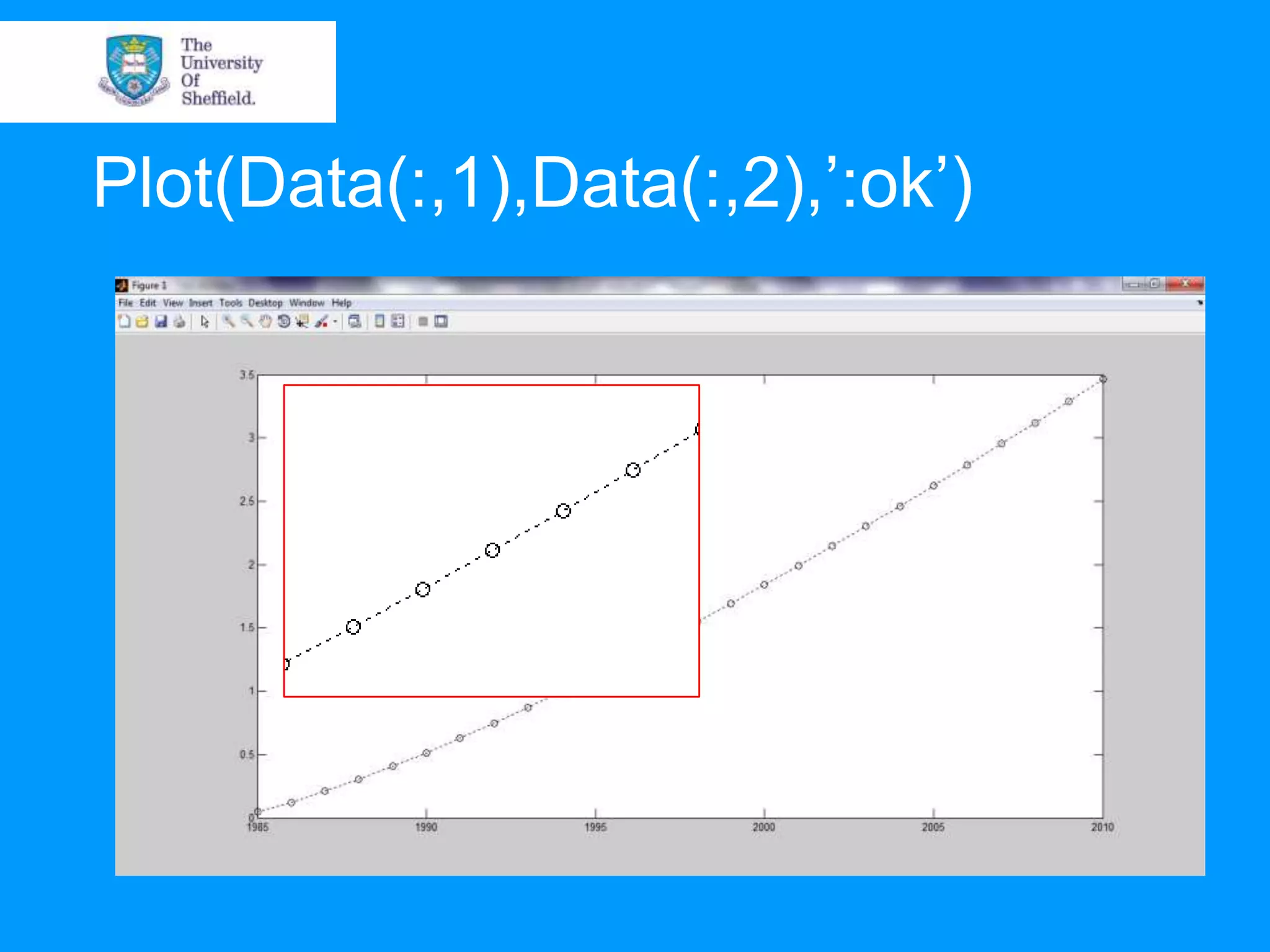
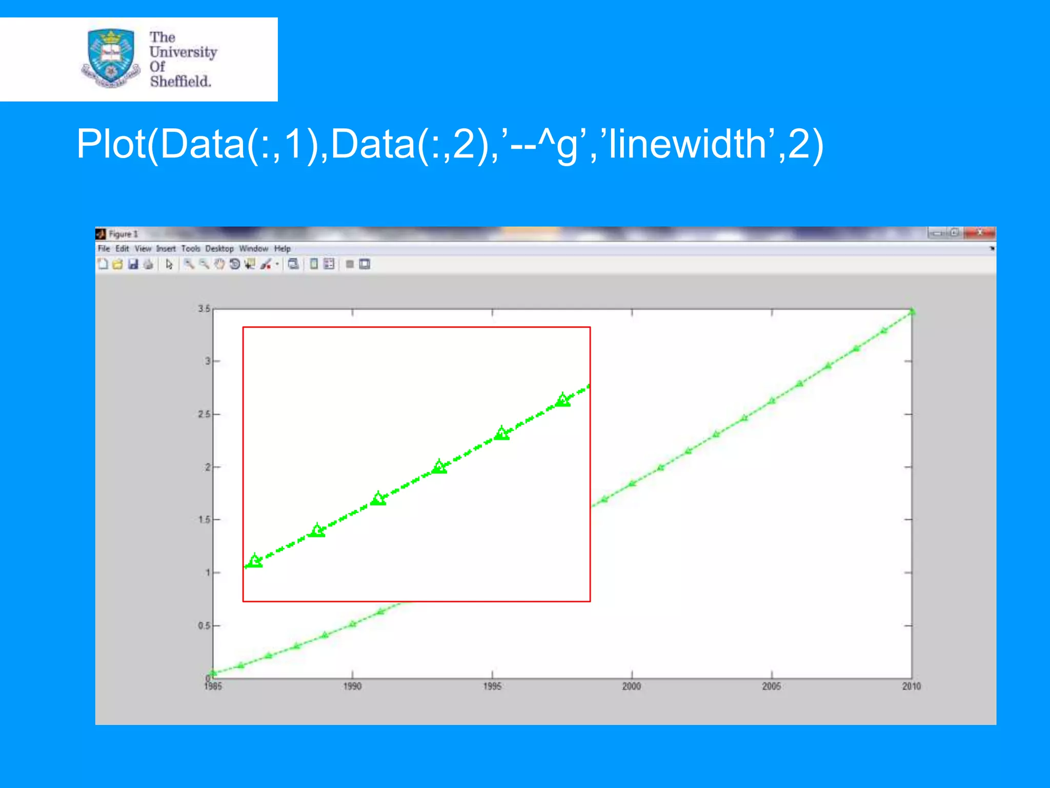
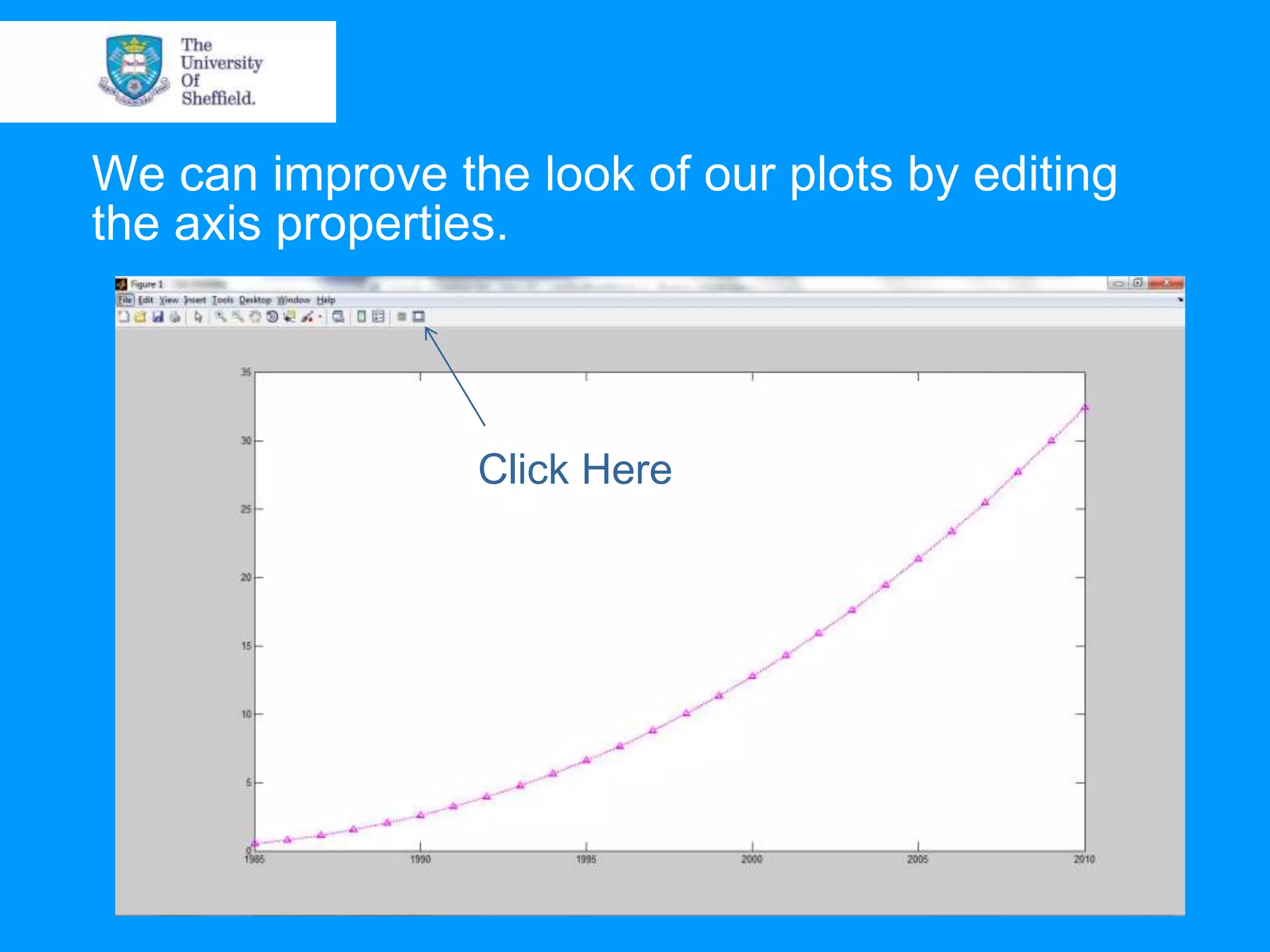
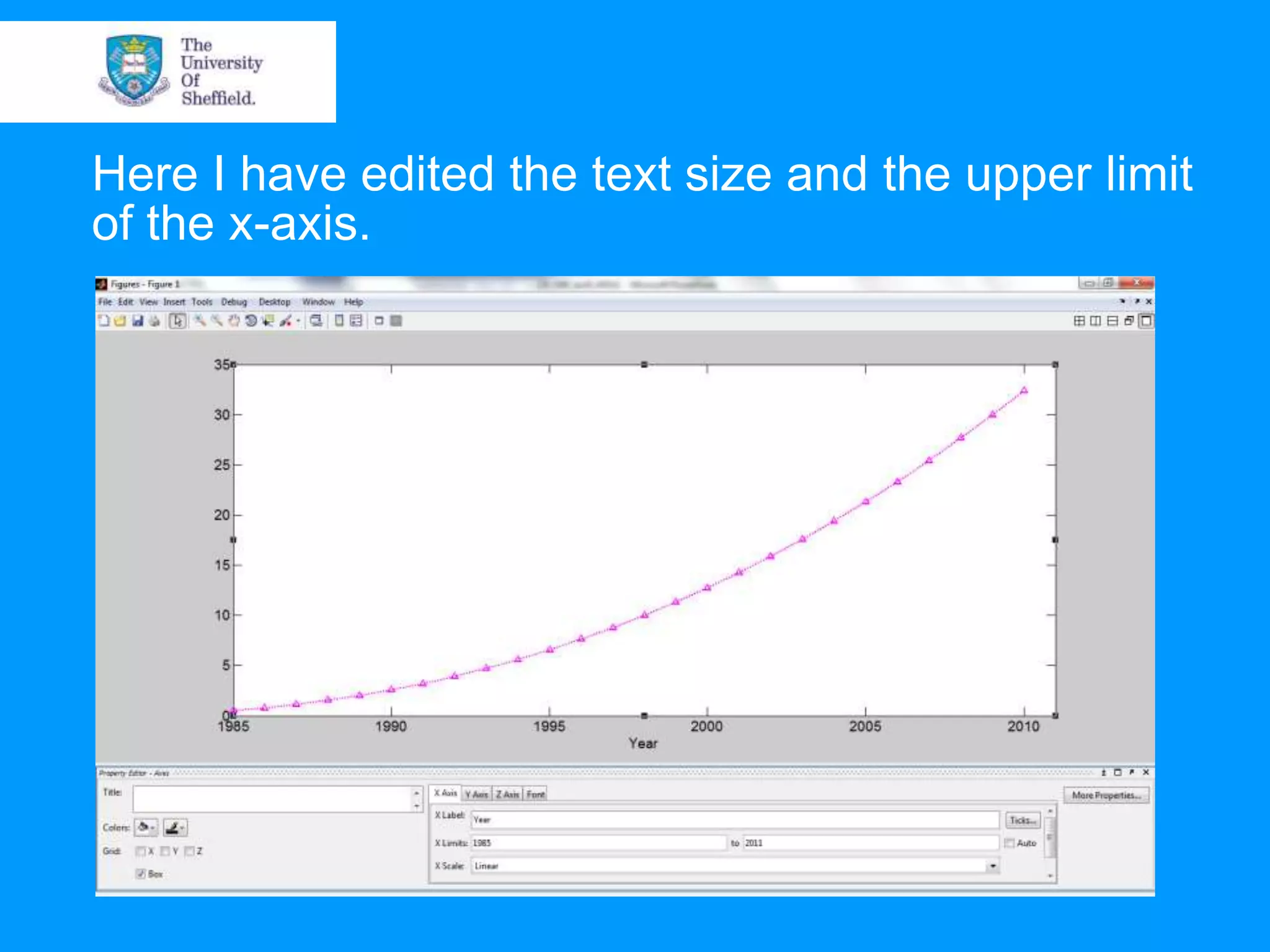
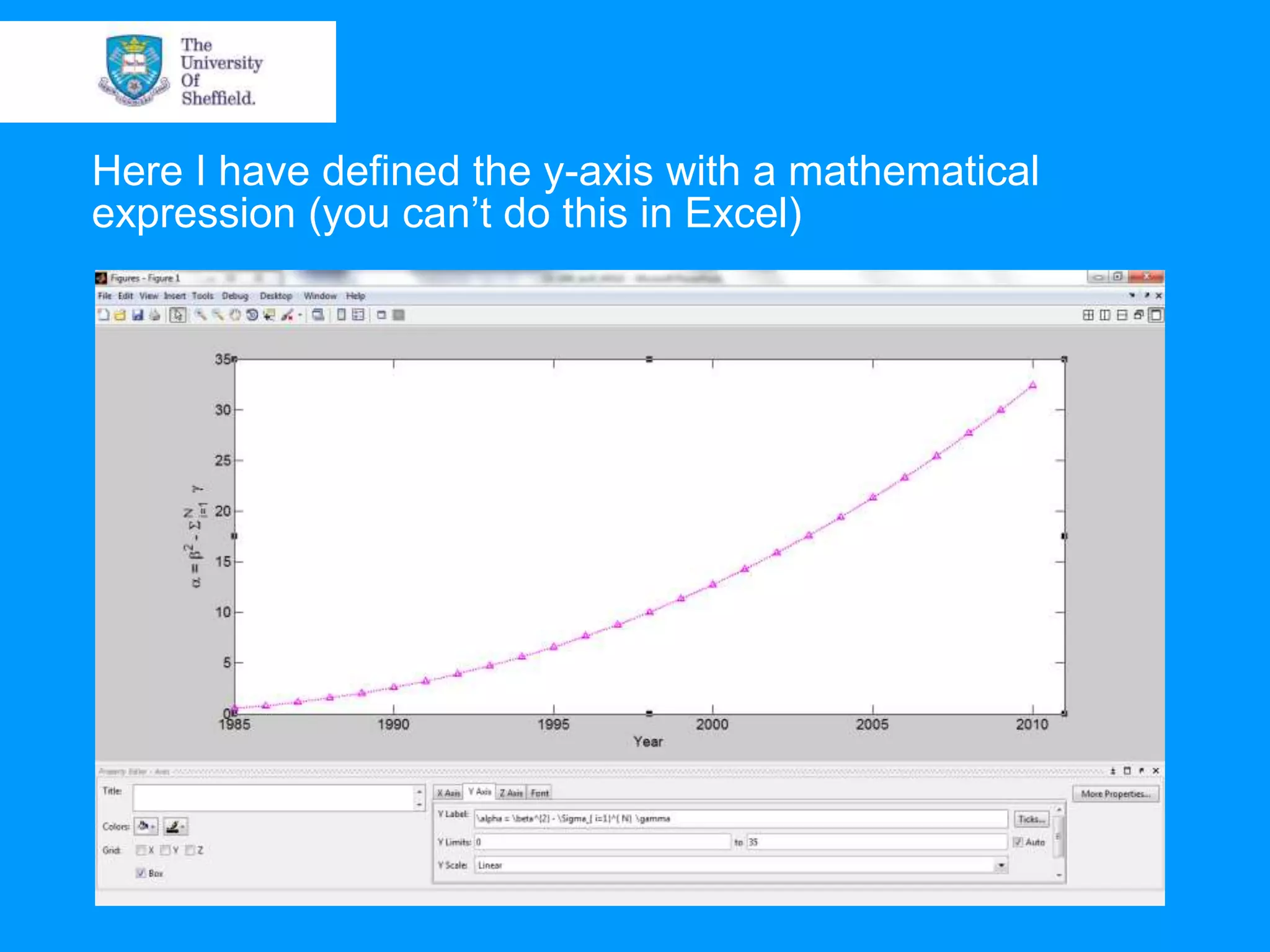
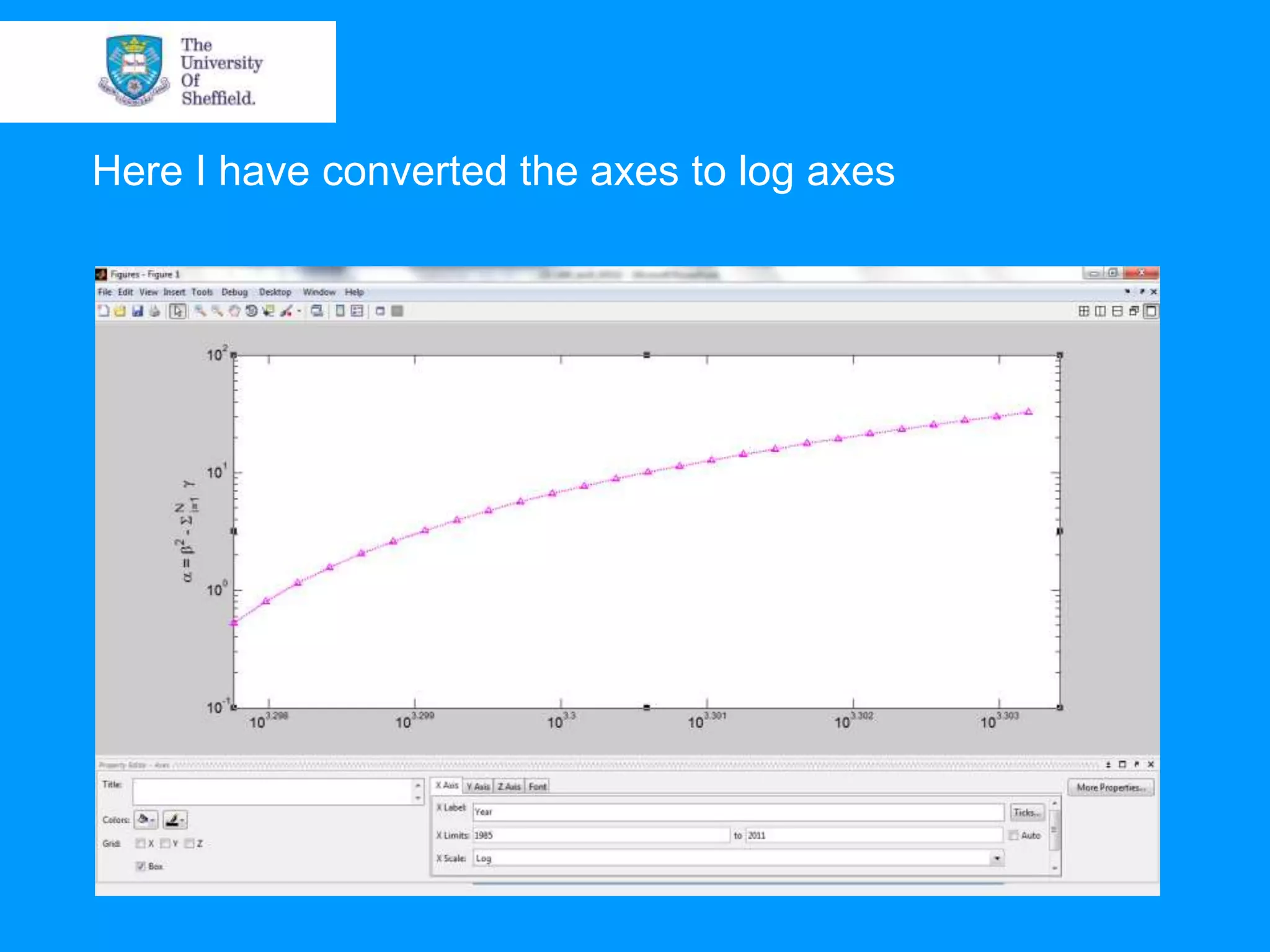
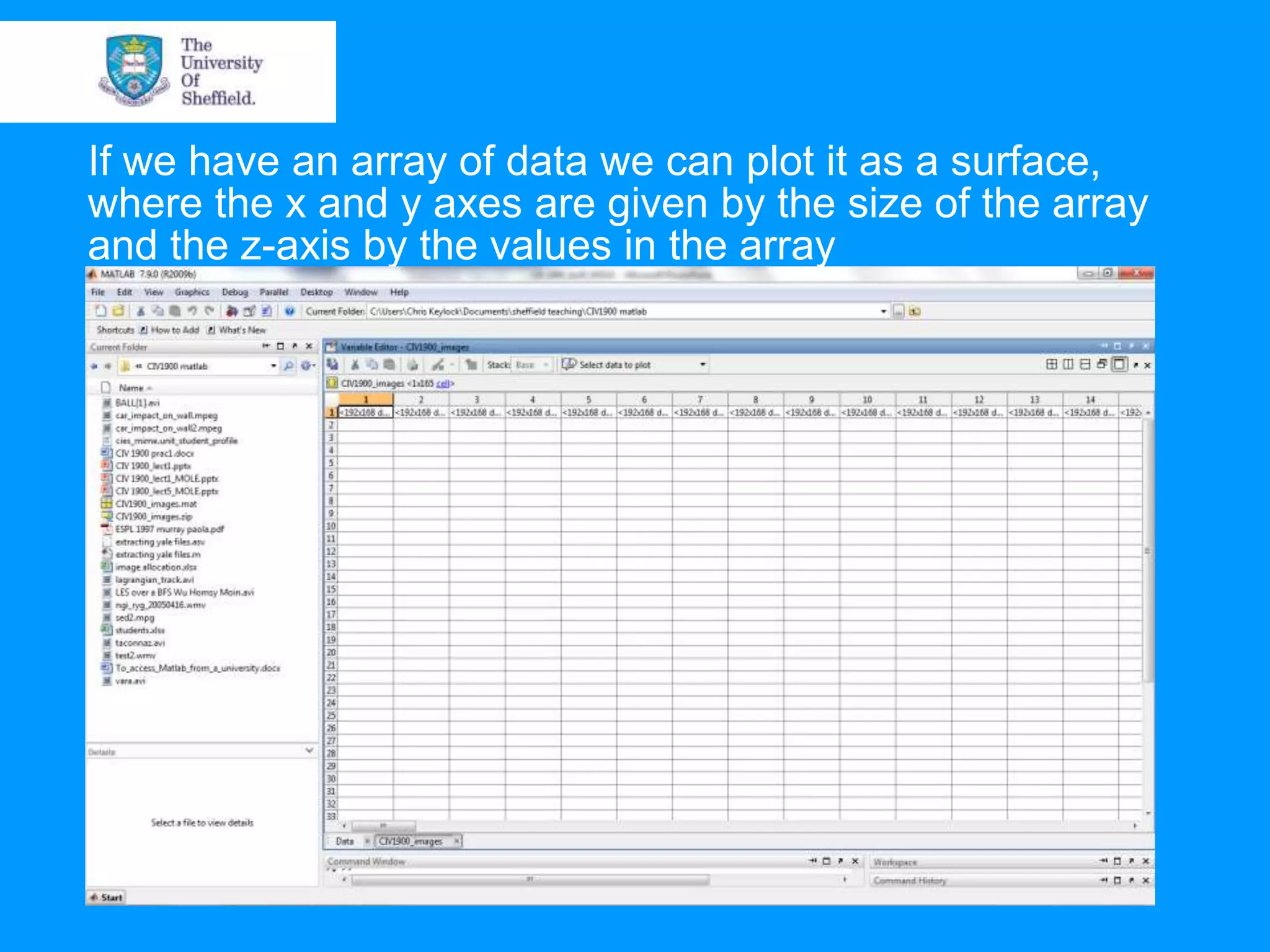
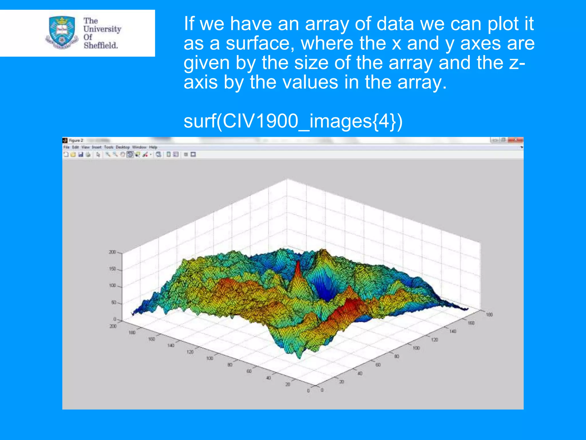
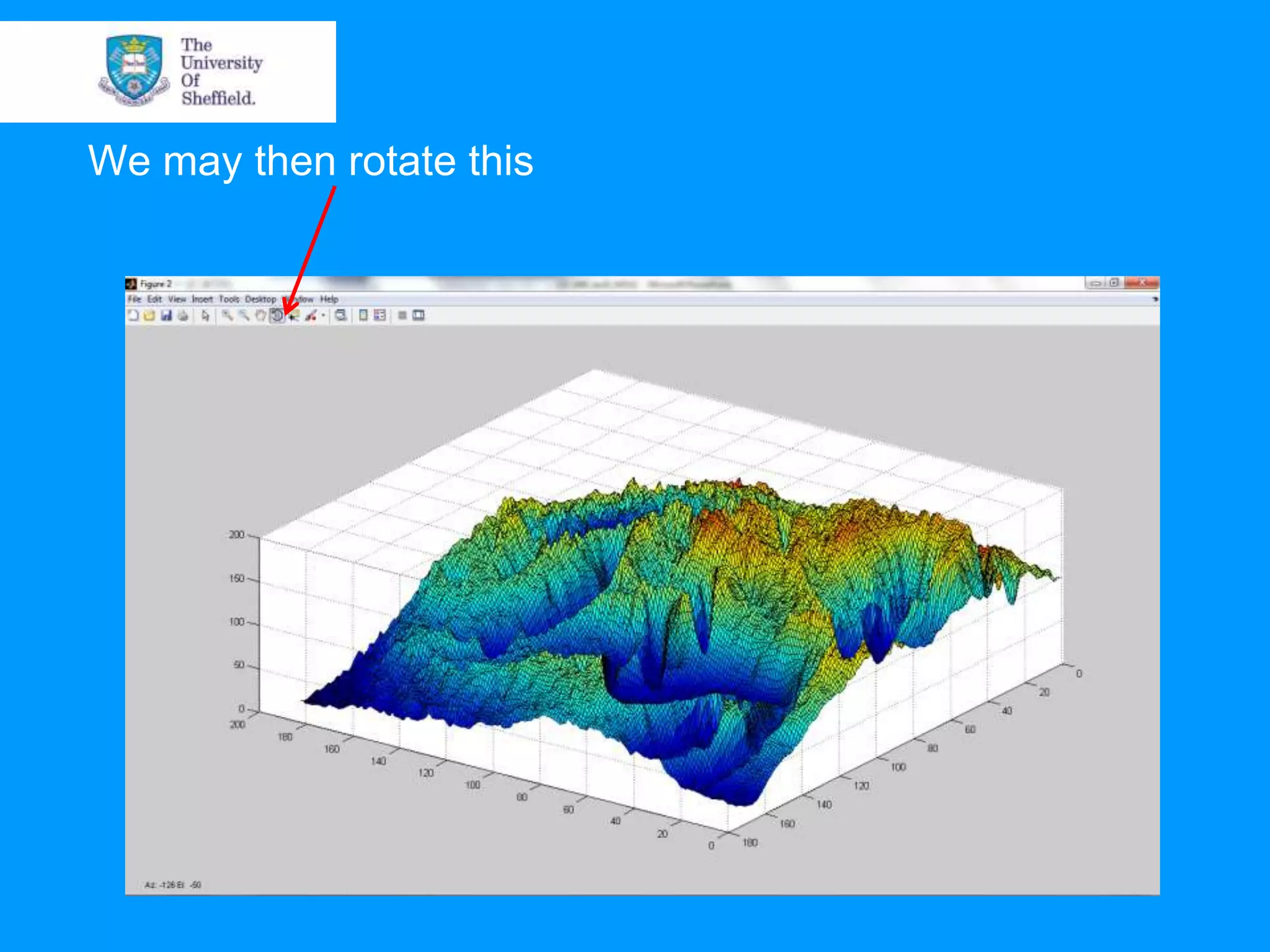
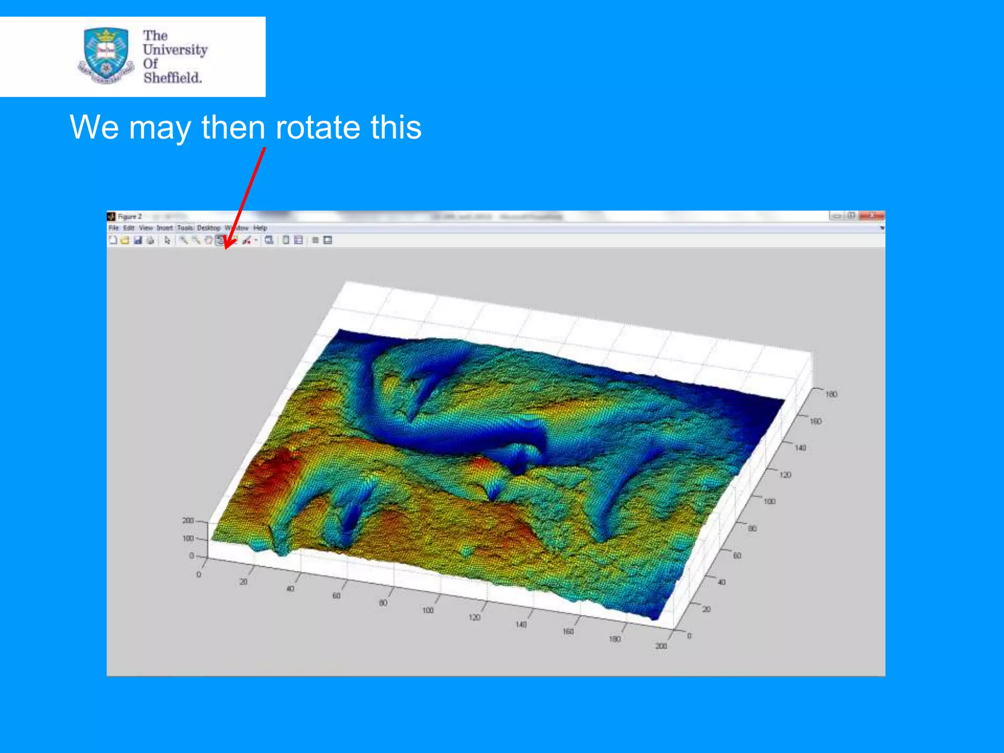
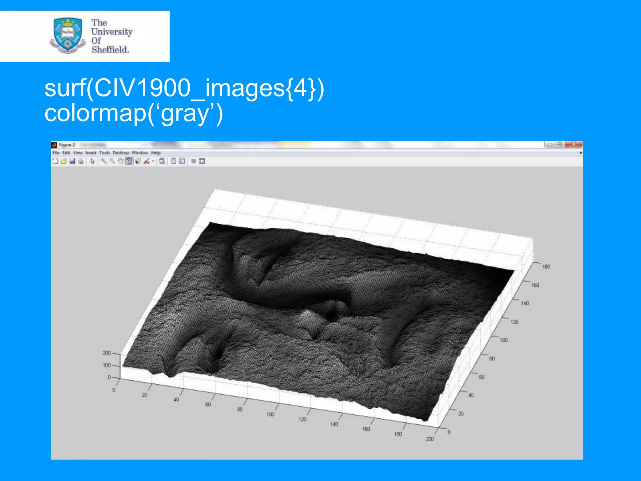
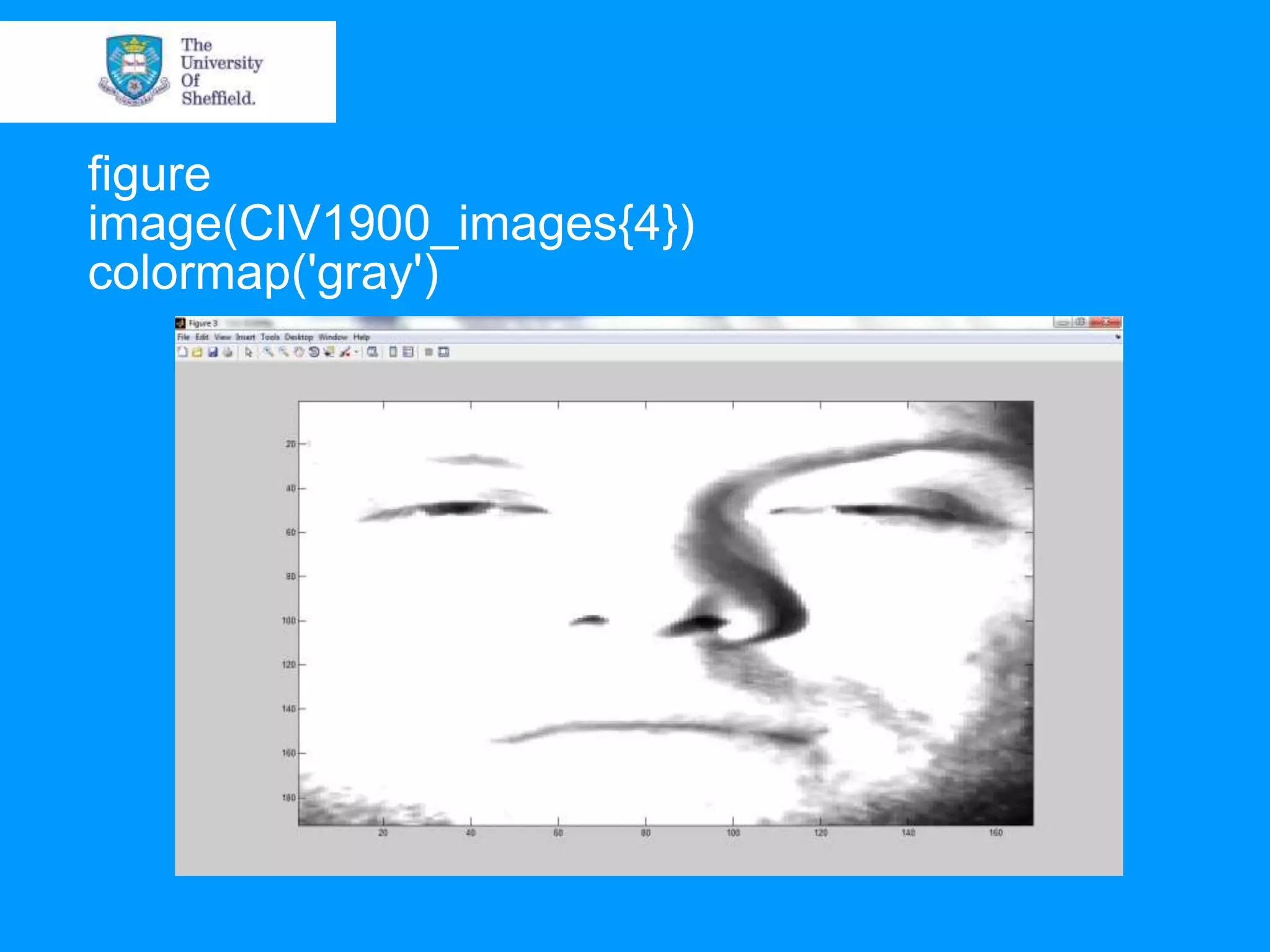
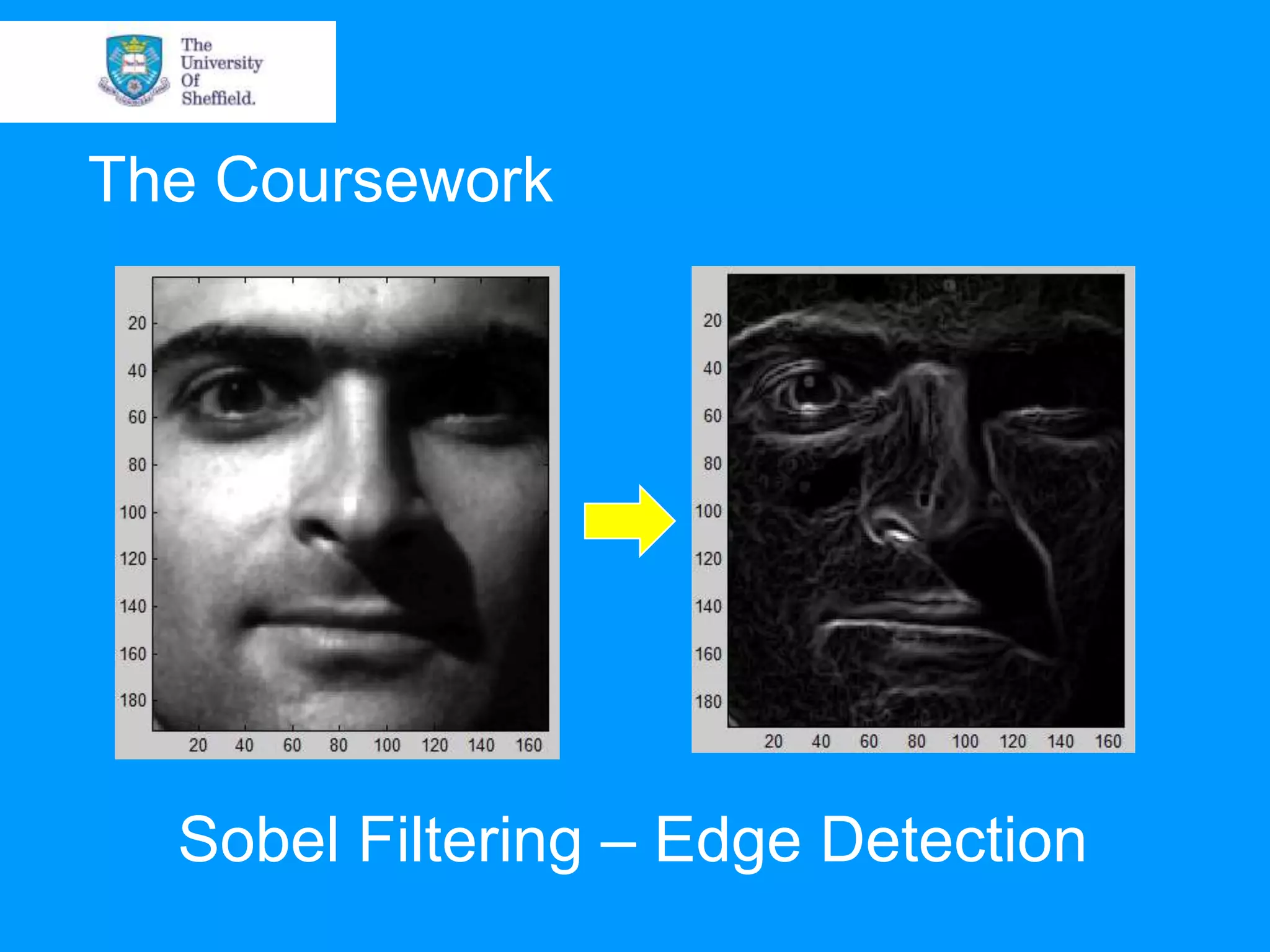
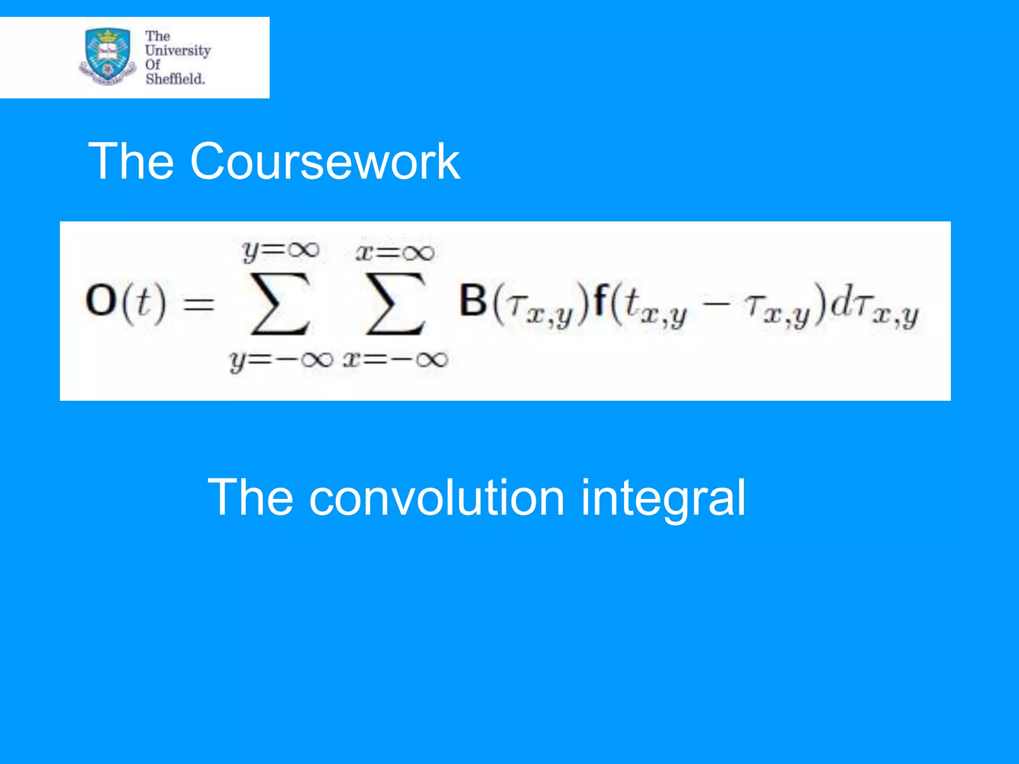
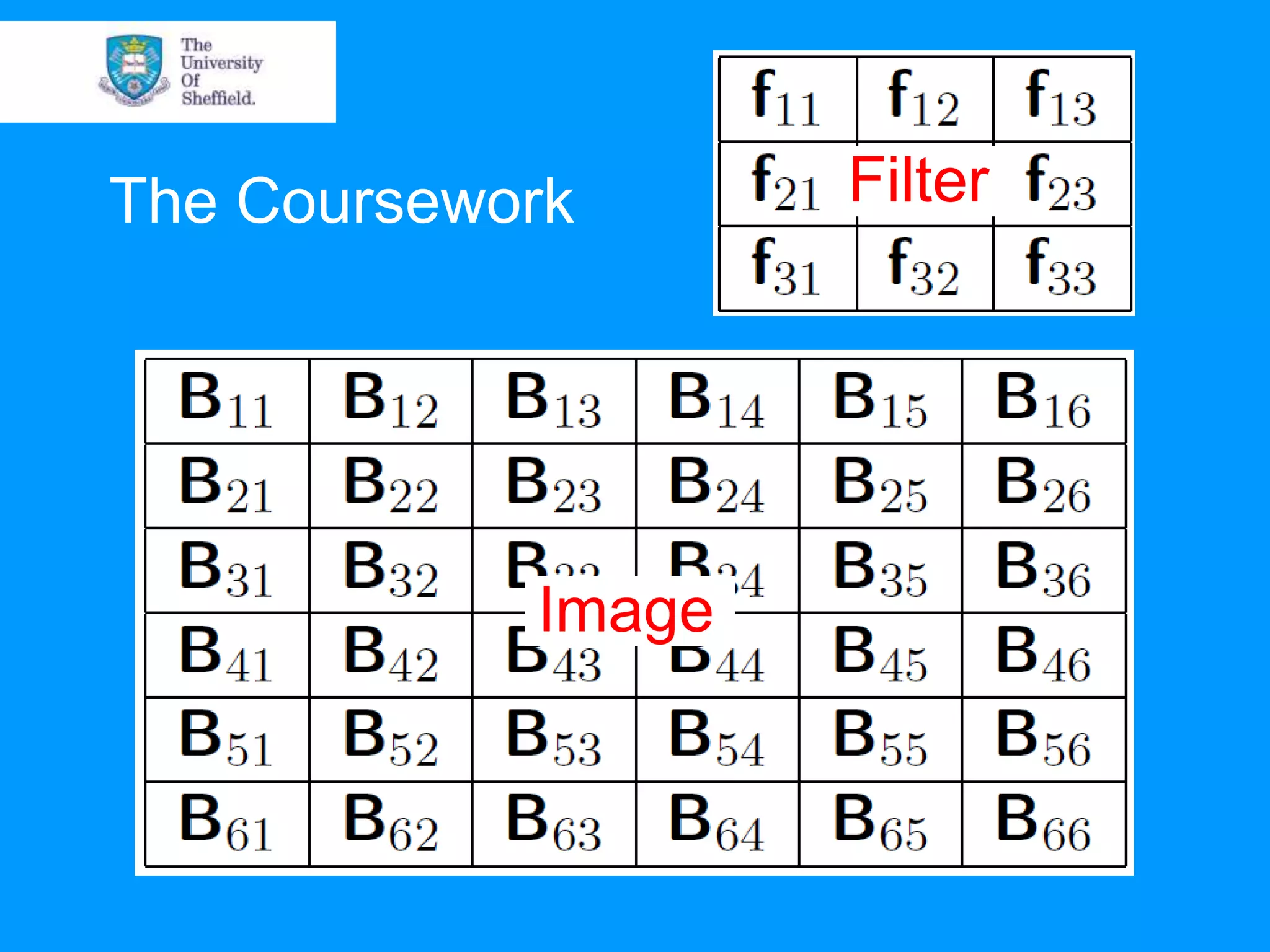
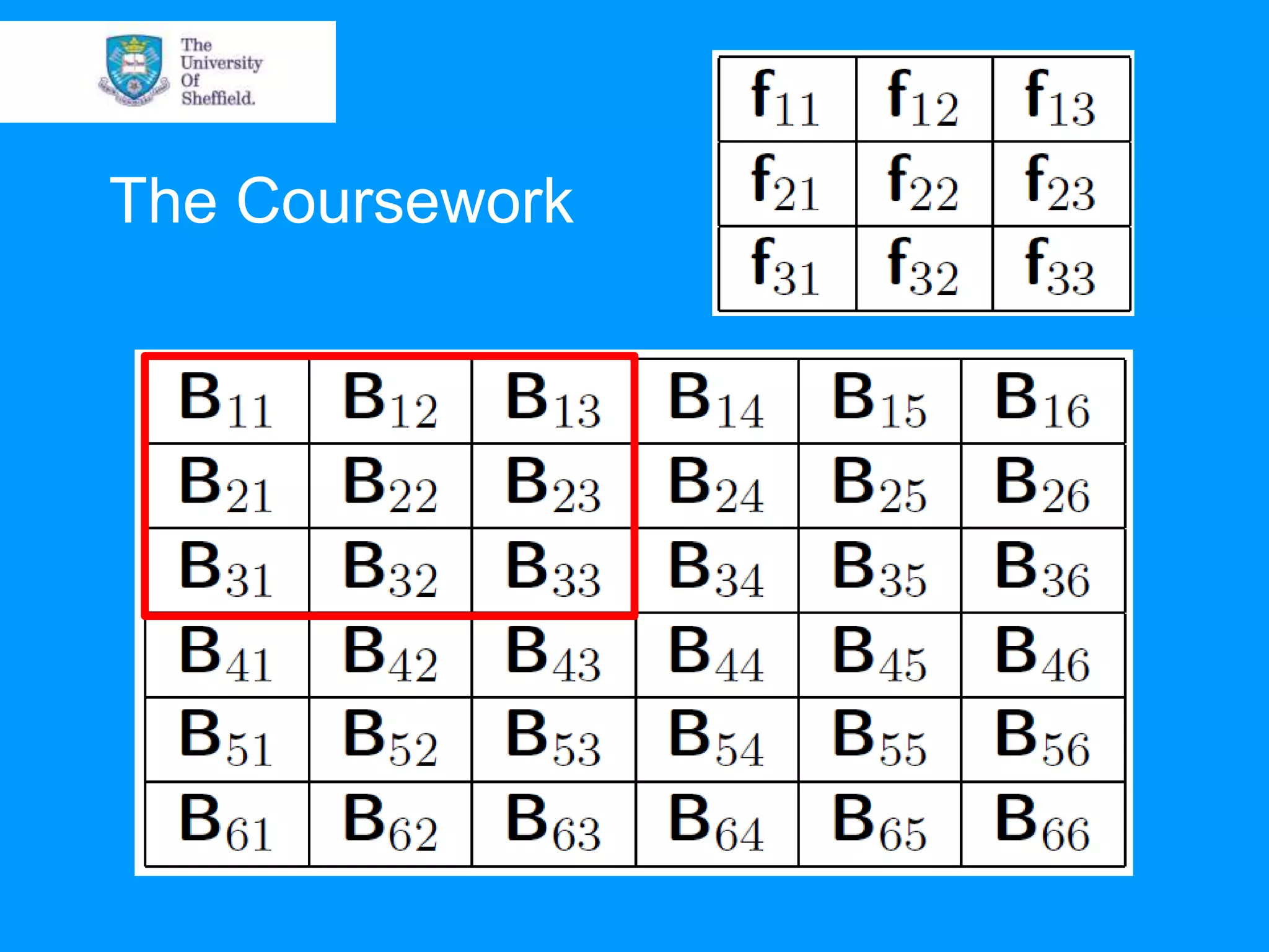
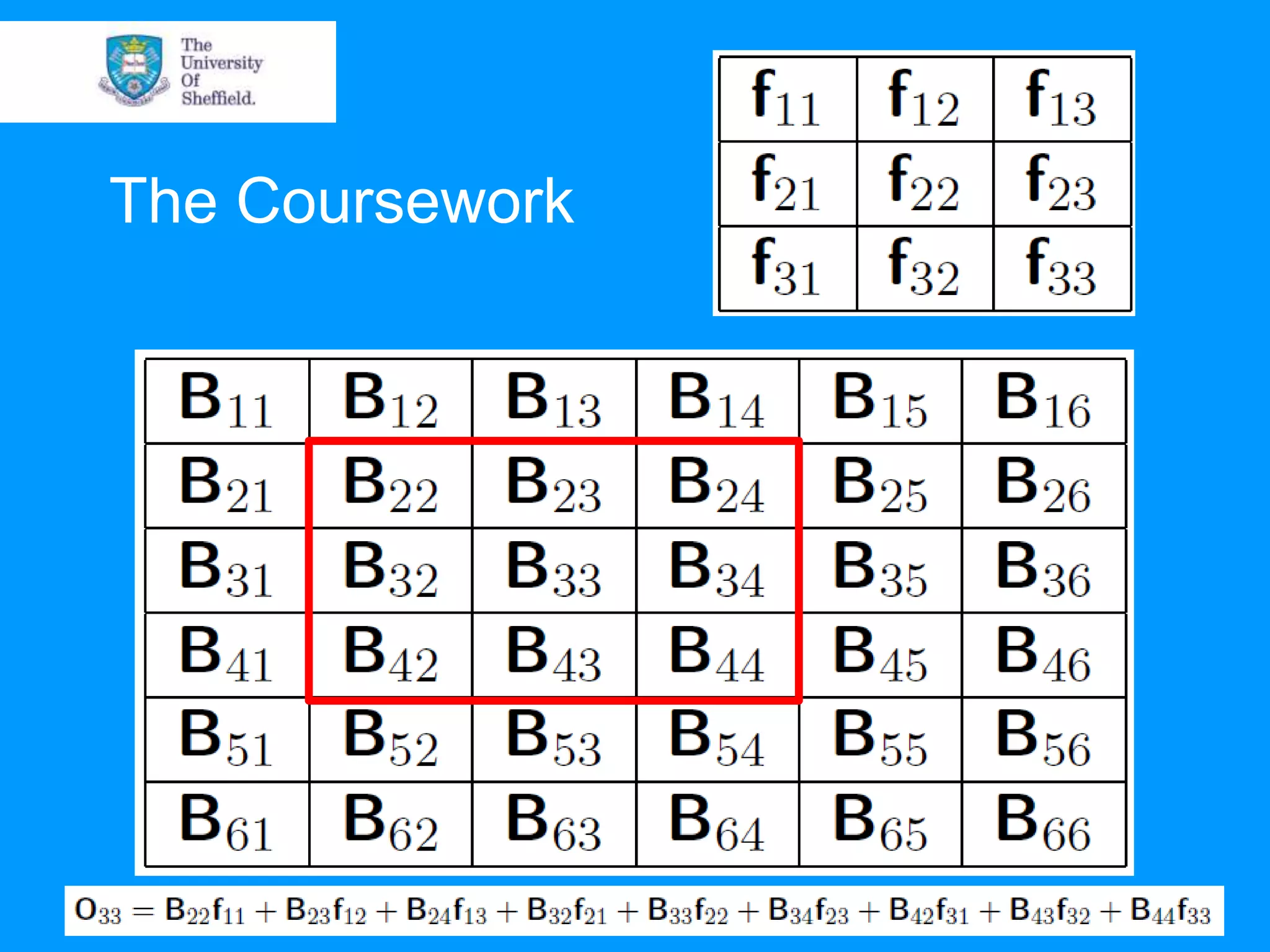
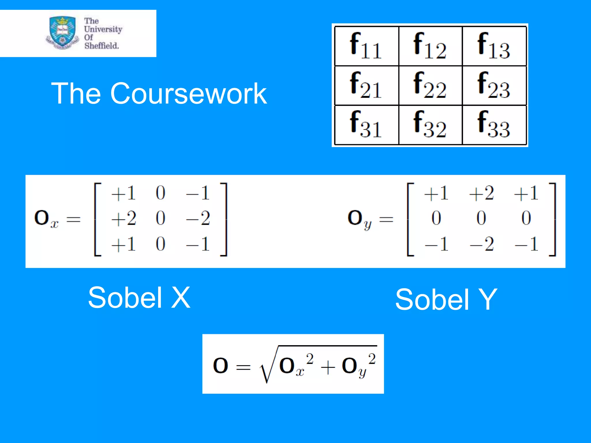
CIV 1900 Computer programming
Contents for Lecture 5 • Plotting capabilities in Matlab • Digital images and their construction • Image processing
Matlab offers a rich graphics environment and even if you do not feel comfortable programming in Matlab you should make use of its graphics capabilities as it will allow you to produce much higher quality graphs and figures than is possible in Excel, for example.
Pressure on the rib and in its lee
Turbulent kinetic energy
The most basic function you can use is to generate scatterplots. Imagine that you have an array of data where the first column contains the year (1985-2010) in which a sample was taken and the second is some property of that sample. A basic piece of exploratory data analysis would be to plot these data against one another.
The Matlab command is “plot” i.e. plot(Data(:,1),Data(:,2)) This defaults to producing a solid line in blue
plot(Data(:,1),Data(:,2)) We can make use of a shorthand for line symbols, line colours and line types to vary this. Some examples: Colours Types Symbols b = blue - = solid line o = circles r = red : = dotted s = square k = black -- = dashed d = diamond g = green ^ = triangle
Plot(Data(:,1),Data(:,2),‟:ok‟)
Plot(Data(:,1),Data(:,2),‟--^g‟,‟linewidth‟,2)
We can improve the look of our plots by editing the axis properties. Click Here
Here I have edited the text size and the upper limit of the x-axis.
Here I have defined the y-axis with a mathematical expression (you can‟t do this in Excel)
Here I have converted the axes to log axes
figure plot (Data(:,1),Data(:,2),':^m','linewidth',1.5) hold on plot (Data(:,1),Data(:,3),„--m','linewidth',1.5)
figure subplot(1,3,1:2) plot (Data(:,1),Data(:,2),':^m','linewidth',1.5) subplot(1,3,3) plot (Data(:,1),Data(:,3),„--m','linewidth',1.5)
A 3D line plot: figure plot3(Data(:,1),Data(:,2),Data(:,3),‟k‟,‟linewidth‟,2)
If we have an array of data we can plot it as a surface, where the x and y axes are given by the size of the array and the z-axis by the values in the array
If we have an array of data we can plot it as a surface, where the x and y axes are given by the size of the array and the z- axis by the values in the array. surf(CIV1900_images{4})
We may then rotate this
Images may also be displayed using the “image” or “imagesc” commands. Hopefully the previous example has highlighted that an image is simply an array of digital numbers. This example was coloured but it was a “false colour” image. There was only level to the array and the colouring was applied in bands: high values (peaks) in red; low values (troughs) in blue. It might as well be a grey-scale image and we can make it so by changing the “colormap”.
surf(CIV1900_images{4}) colormap(„gray‟)
A “true colour” image (like a jpeg file) is constructed rather differently. Instead of a single layer to the array, it has layers for each colour: Three layers for an RGB image Four for a CMYK image Each layer ranges from 0 to 255 and tells you how red or green or blue the colour is at that point. When they are all combined they give you the colour at that location, which using a legend, you can relate to properties of the image.
Colour maps in Matlab by default range from 0 to 63. The “image” command displays an image literally relating the values in the array to the colour map. The “imagesc” command rescales the values in the array so that they fit the colour map. For example, the values in our image go from 0- 255 so using “image” we would expect about 75% of the image to wash out as white
figure image(CIV1900_images{4}) colormap('gray')
figure imagesc(CIV1900_images{4}) colormap('gray')
figure imagesc(CIV1900_images{4}) axis („image‟) colormap('gray')
figure for loop1=1:9 subplot(3,3,loop1) imagesc(CIV1900_images{loop1*3+4}) axis image colormap('gray') end
Matlab provides a flexible tool for producing graphics. This includes images, which are simply arrays of numbers (1 layer for grey-scale, more for true colour). Image processing is an important area of engineering science: Stress analysis on beams using photostress systems; Particle Imaging velocimetry; Monitoring of land use change using remote sensing; Face or fingerprint recognition software, etc.
The Coursework Sobel Filtering – Edge Detection
The Coursework The convolution integral
The Coursework Filter Image
The Coursework
The Coursework
The Coursework Sobel X Sobel Y

CIV1900 Matlab - Plotting & Coursework