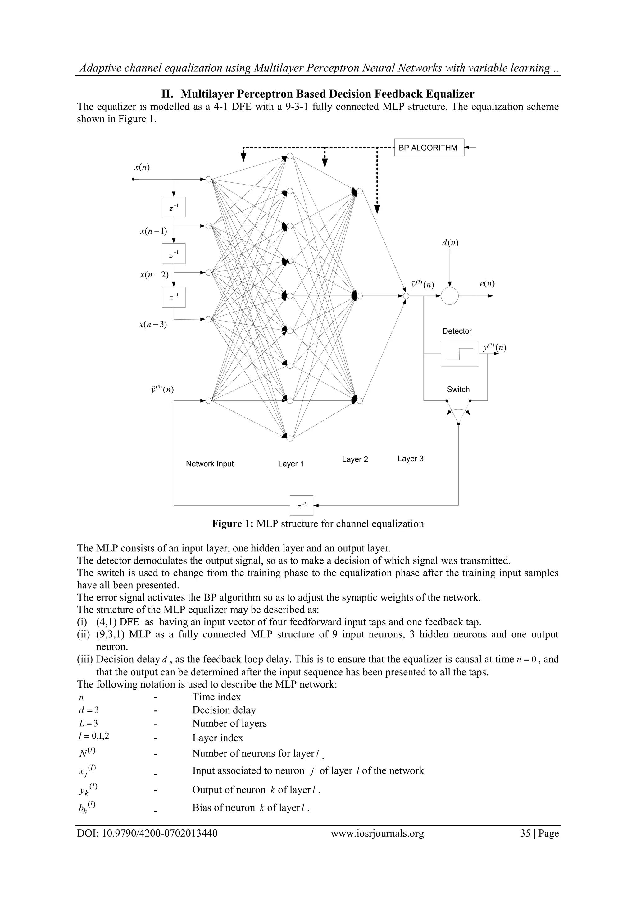
IOSR Journal of VLSI and Signal Processing (IOSR-JVSP) Volume 7, Issue 2, Ver. I (Mar. - Apr. 2017), PP 34-40 e-ISSN: 2319 – 4200, p-ISSN No. : 2319 – 4197 www.iosrjournals.org DOI: 10.9790/4200-0702013440 www.iosrjournals.org 34 | Page Adaptive Channel Equalization using Multilayer Perceptron Neural Networks with variable learning rate parameter Emmanuel K. Chemweno1 , Edward. N. Ndung’u2 , Heywood A. Ouma3 1 (Dept. of Telecommunications and Information Engineering, Jomo Kenyatta University of Agriculture and Technology, Box 62000, Nairobi , Kenya) 2 (Dept. of Telecommunications and Information Engineering, Jomo Kenyatta University of Agriculture and Technology, Box 62000, Nairobi , Kenya) 3 (Dept. of Electrical and Information Engineering, University of Nairobi, Box 30197, Kenya) Abstract: This research addresses the problem inter-symbol interference (ISI) using equalization techniques for time dispersive channels with additive white Gaussian noise (AWGN). The channel equalizer is modelled as a non-linear Multilayer Perceptron (MLP) structure. The Back Propagation (BP) algorithm is used to optimize the synaptic weights of the equalizer during the training mode. In the typical BP algorithm, the error signal is propagated from the output layer to the input layer while the learning rate parameter is held constant. In this study, the BP algorithm is modified so as to allow for the learning rate to be variable at each iteration and this achieves a faster convergence. The proposed algorithm is used to train the MLP based decision feedback equalizer (DFE) for time dispersive ISI channels. The equalizer is tested for a random input sequence of BPSK signals and its performance analysed in terms of the Bit Error Rates and speed of convergence. Simulation results show that the proposed algorithm improves the Bit Error Rate (BER) and rate of convergence. Keywords: Equalization, intersymbol interference, multilayer perceptron, back propagation, variable learning rate, bit error rate (BER) I. Introduction Real physical channels suffer the problem of signal degradation due to AWGN, time dispersive channels and multipath propagation [1], [2]. This causes the received pulses to smear onto each other with the result that they are no longer distinguishable [3].This is known as ISI and has the effect of reducing the rate of data transmission over a communication channel. Channel equalization is used to mitigate the effects of ISI. In most channels, the characteristics vary with time, and an adaptive equalizer whose coefficients vary automatically and adaptively is desirable [1], [4]. Traditionally, equalizers were modelled as linear equalizers using finite impulse response (FIR) transversal or lattice structure filters. These used the least mean square error (LMS) and recursive least square error (RLS) algorithms to optimise the equalizer coefficients. These algorithms do not perform well for channels with non- linearities and is never used for non-minimum phase channels [5]. Decision feedback equalizer (DFE) is non- linear and yields superior results to a linear equalizer [1] and is used to mitigate ISI in non-linear channels provided the distortion is not too severe. The DFE, however, suffer the problem of error propagation [6]. Neural networks (NN) perform well for non-linear channels [7] and are used for both minimum and non-minimum phase channels and are resistant to additive noise [8]. NN are complex and exhibit slower learning times than linear equalizers [6]. In order to minimize the computational complexity and accelerate the slow learning process (convergence rate), modification of the learning algorithms has been proposed. Lee et al [9] have proposed a hierarchical topology of the MLP, where, each layer has got its own BP algorithm and the results were superior to that of the standard BP algorithm.
Adaptive channel equalization using Multilayer Perceptron Neural Networks with variable learning .. DOI: 10.9790/4200-0702013440 www.iosrjournals.org 35 | Page II. Multilayer Perceptron Based Decision Feedback Equalizer The equalizer is modelled as a 4-1 DFE with a 9-3-1 fully connected MLP structure. The equalization scheme shown in Figure 1. 3 z 1 z 1 z 1 z )(nx )3( nx )2( nx )1( nx )()3( ny  BP ALGORITHM )(nd )(ne )()3( ny )()3( ny  Detector Network Input Layer 1 Layer 2 Layer 3 Switch Figure 1: MLP structure for channel equalization The MLP consists of an input layer, one hidden layer and an output layer. The detector demodulates the output signal, so as to make a decision of which signal was transmitted. The switch is used to change from the training phase to the equalization phase after the training input samples have all been presented. The error signal activates the BP algorithm so as to adjust the synaptic weights of the network. The structure of the MLP equalizer may be described as: (i) (4,1) DFE as having an input vector of four feedforward input taps and one feedback tap. (ii) (9,3,1) MLP as a fully connected MLP structure of 9 input neurons, 3 hidden neurons and one output neuron. (iii) Decision delay d , as the feedback loop delay. This is to ensure that the equalizer is causal at time 0n , and that the output can be determined after the input sequence has been presented to all the taps. The following notation is used to describe the MLP network: n - Time index 3d - Decision delay 3L - Number of layers 2,1,0l - Layer index )(l N - Number of neurons for layer l . )(l jx - Input associated to neuron j of layer l of the network )(l ky - Output of neuron k of layer l . )(l kb - Bias of neuron k of layer l .
Adaptive channel equalization using Multilayer Perceptron Neural Networks with variable learning .. DOI: 10.9790/4200-0702013440 www.iosrjournals.org 36 | Page )(l kjw - The synaptic weight connecting to the input of neuron k of layer l to output j of layer 1l to )2( kd - Target output k of the output layer. )( - Activation function III. Proposed Algorithm To increase the speed of the LMS algorithm without using estimates of the input signal correlation matrix, variable convergence factor is desirable. The proposed algorithm is developed from the Normalised Least Mean Square (NLMS) algorithm which is expressed by equation (1): )( )( )( )()1( 2 ne n n nn x x ww   (1) Where: )(nw  = Filter weight vector at time n )(nx = Input signal vector  = Learning rate parameter )()()( nyndne  ; The error between the desired output and the actual output In order to make the learning rate parameter adaptive, the NLMS weight update equation given by equation (1) is re-written as equation (2): )( )( )( )()()1( 2 ne n n nnn x x ww   (2) Where: )(n = The learning rate parameter at time n Defining the weight error vector as the difference between the unknown true filter weight vector tw and the filter weight at given time )(nw  : )()( nn t wwε   (3) )( )( )( )()()1()1( 2 ne n n nnnn t x x εwwε   (4) To minimize the mean square error (MSE), the expectations of the squared norms of equation (4) is taken: })( )( )( )()({})1({ 2 2 2 ne n n nnEnE x x εε  = })({ 2 nE ε )(n (5) Where: )( )()( )( )({)(2})( )()( )()( )({)()( 2 2 n nn n neEnne nn nn neEnn T T T T ε xx x xx xx   (6) To maximize )(n , we make it the objective function and differentiate with respect to , and equate to zero. 0)( )()( )( )({2})( )()( )()( )({)(2 )( 2   n nn n neEne nn nn neEn d nd T T T T ε xx x xx xx    (7) And })( )()( )()( )({ })( )()( )( )({ )( 2 ne nn nn neE n nn n neE n T T T T o xx xx ε xx x  (8) Where: )(no = The optimum step size at time n
Adaptive channel equalization using Multilayer Perceptron Neural Networks with variable learning .. DOI: 10.9790/4200-0702013440 www.iosrjournals.org 37 | Page To make the computation of )(no tractable, the fluctuations of the input signal energy )()( nnT xx is assumed to be small from one iteration to the next such that equation (8) may be simplified to [3] : })({ )}()()({ })()({ )}()()()({ })()({ )}()()({ })( )()( )()( )({ })( )()( )( )({ 2 2 2 neE nnneE nnE nennneE nnE nnneE ne nn nn neE n nn n neE T T T T T T T T T εx xx xx xx εx xx xx ε xx x  (9) We introduce apriori error vector such that ae is given by[10]: )()()()( nnndne T a wx )()()()()( nnnnnd T t T εxwx  (10) The desired signal )(nd is given by equation (10). )()()( nnnd t T wx , (11) Therefore: )()()( nnne T a εx ` (12) The error vectors )(ne are related to the apriori error vector by: )()()( nvnene a  )()()( nvnnT  εx (13) Where: )(nv = Noise Replacing equation (13) in into equation (9), and neglecting the dependency of )(nε on the past noise [3],[10], reduces equation (9) to: })()()()(2)()()()({ )}()()({)}()()()({ )( 2 nvnvnnnnnnE nnnvEnnnnE n TTT TTT o    εxεxxε εxεxxε  (14) For Gaussian signals 0)]([ nvE and 22 ])([ nvE })()()()({ )}()()()({ )( 2     nnnnE nnnnE n TT TT o εxxε εxxε (15) The term )]()()()([ nnnnE TT εxxε in equation (15) may be further simplified as: )]()}()({)([)]()()()([ nnnEnEnnnnE TTTT εxxεεxxε  )]()([)]()()()([ nnEnnnnE TTT Rεεεxxε  (16) Where: )]()([ nnE T xxR  the correlation matrix By using the diagonalized form of T QQR (17)  )]()([)]()([)]()([ nnEtrnnEnnE TTTT Λε'ε'εΛεRεε  QQ (18) Where: Q = Eigen vector matrix of the correlation R Λ = Eigen values of R ][tr = Trace operation )()( nn T εε' Q (19) The effect of the transformation )(nt wwε   shifts the error performance contours from the w  axes to the ε axes. The transformation )()( nn T εε' Q rotates the contours such that the principal axes of the ellipses are aligned with the ε' axes without altering the shape or eccentricity of the performance surface. The solution for equation (18) is given by [3]:       1 0 2 )(')]()([ N k kkk T nnnEtr Λε'ε' (20)
Adaptive channel equalization using Multilayer Perceptron Neural Networks with variable learning .. DOI: 10.9790/4200-0702013440 www.iosrjournals.org 38 | Page Where: kk' are the diagonal elements of the matrix )(nε' k are the corresponding eigen values In developing the proposed algorithm, the following assumptions are made: (i) The assumption made in equation (9) that the input data signal matrix is stationary in the wide sense is extended here. Therefore, the changes in Q and Λ are negligible over a block of data input. This aims at minimizing computational complexity. (ii) To recursively compute equation (20), the following approximation is made:         1 0 2 1 0 2 )(')(')]1()1([ N k kkk N k kkk T nnnnEtr ε'ε' (21) Where: )(n = Change in the weight error vector The choice of the sign will depend on the error gradient )1()( nxne . Successive changes in sign of this quantity indicates that the algorithm is close to its optimal and must the learning rate parameter should be reduced. (i) After the first transformation, the MSE contours are aligned on the principal axes such that )()(' nn εε  . Successive contours are very close to each other along the main axis. The rotation transformations of the weight error matrix change )(nε are avoided for the subsequent data inputs in a block. The signal power is normalized and noise variance 2  in equation (15) be approximated as SNR L [10]. (22) Where: L = Number of taps of a discrete filter model of the channel The variable step size algorithm of equation (15) may therefore re-written as: SNR L n N k kkk N k kkk o         1 0 2 1 0 2 ' ' )(    ;0n (23) SNR L nn nn n N k kkk N k kkk N k kkk N k kkk o              1 0 2 1 0 2 1 0 2 1 0 2 )()(' )()(' )1(    ;0n (24) IV. Equalization Process A random input of BPSK modified information sequence )(nI is passed through a time dispersive channel with AWGN. The equalization process takes place in two phases: the training phase and the decision directed phase. During the training phase the input to the MLP network is a vector consisting of a time delayed input sequence and the undetected feedback signal defined as: T nynxnxnxnxn )]3(),3(),2(),1(),([)( )3(   x (25) During this phase, the output of the MLP network is computed layer by layer from the input to the output. The error is backpropagated from the output layer to the input layer, for the adjustments of the weights. After the training phase, the equalizer switches to the decision directed mode, whereby the feedback signal is the detected version of the output )(ny . V. Simulation Results The proposed algorithm was simulated for a channel model given by the impulse response: 21 3842.08704.03482.0)(   zzzH (26) This channel is non linear in nature and has been cited extensively in literature and is recommended by International Telecommunication Union (ITU) for testing equalizers The performance criteria used to evaluate the performance of the algorithm was the quality of convergence and the bit error rate. In the quality of convergence criteria, an average of 5000 individual runs, each having a sequence of 2500 random signals was used. Figure 2 shows the simulation results plotted against the standard back propagation algorithm (BP) and the modified back propagation (HBP) algorithm [9].
Adaptive channel equalization using Multilayer Perceptron Neural Networks with variable learning .. DOI: 10.9790/4200-0702013440 www.iosrjournals.org 39 | Page The MATLAB® BER template is used to determine the BER, whereby multiple runs is made with different data inputs. SNR is varied from 0 to 25 dB. At each SNR, the process of equalization is carried out until either a target number of 100 errors are observed, or when the equalizer has processed a maximum of 100,000 bits. The first 1000 symbols were used for training the MLP, with the remaining 1500 to test the performance. Figure 3 shows the BER performance for the BP, HBP [9] and the proposed algorithm, plotted on the same axes. 0 5 10 15 20 25 10 -6 10 -5 10 -4 10 -3 10 -2 10 -1 10 0 BER comparison for three algorithms SNR BER BP algorithm HBP algorithm Proposed algorithm Figure 2: BER Comparison for three algorithms 0 500 1000 1500 2000 2500 10 -2 10 -1 10 0 10 1 Learning curve for MSE for three different algorithms for SNR = 20dB Number of iterations MSE[dB] BP algorithm HBP algorithm Proposed algorithm Figure 3: Learning curves for the three algorithms
Adaptive channel equalization using Multilayer Perceptron Neural Networks with variable learning .. DOI: 10.9790/4200-0702013440 www.iosrjournals.org 40 | Page VI. Simulation Results This study presents a variable learning rate algorithm for MLP based DFE equalizer. Results for the standard BP, HBP and the proposed algorithm are plotted on the same axes for comparison and inference. At low SNR where the level of corruption in the transmitted signal is very high, the three algorithms yield approximately the same results. BER performance is also very poor owing to high noise power. As the SNR is increased, the proposed algorithm offers an improved performance and the number of errors in the equalized signal is greatly reduced. The algorithm offers a better classification of the noisy input so as correctly make a decision on which symbol had been transmitted. Furthermore, the proposed algorithm offers a minimum MSE compared to the standard BP and HBP algorithms. Simulation results show that the proposed algorithm offers a better performance in both the BER and the quality of convergence criteria as compared to the standard BP and the HBP algorithms. References [1]. Proakis J. G. Digital communications, 3rd Edition, McGraw-Hill, Inc. 1995 [2]. Paul J. R, Vladimirova T. “Blind equalization with recurrent neural networks using natural gradient”, ISCCSP symposium, March 2008, pp 178-183 [3]. Haykin S., Adaptive Filter Theory, Prentice Hall, 4th Edition, 2002 [4]. Bic J. C., Duponteil D. and Imbeaux, J. C. Principles of communication systems, John Wiley & Sons, 1986 [5]. Pichevar R., Vakili V. T., Channel equalization using neural networks, IEEE, 1999 [6]. Yuhas B, Ansaris N. Neural Networks in Telecommunications, “Neural network Channel Equalization” Kluwer Academic Press, 1994 [7]. Mo S. and Shafai B. “Blind equalization using higher order cumulants and neural networks”, IEEE transaction on signal processing. Vol 42 no. 11, 1994, pp 3309 - 3217 [8]. Wang B. Y. and Zheng W. X., “Adaptive blind channel equalization in chaotic communications by using non linear prediction technique”, IEE proceedings on Visual, image and signal processing, vol 153 no 6, December 2006, pp – 810 - 814 [9]. Lee C. M., Yang S. S. and Ho C. L., “Modified back propagation algorithm applied to Decision feedback equalization”, IEE procedings on visual, image signal processing, vol 153, no. 6, December 2006, pp 805 - 809 [10]. Hadei S. A., Azmi P., Sonbolestam N., Abbasian J., “ Adaptive channel equalization using variable step-size partial rank algorithm based on unified framework”, Proceedings of the ICEE, May 2010

Adaptive Channel Equalization using Multilayer Perceptron Neural Networks with variable learning rate parameter

  • 1.
    IOSR Journal ofVLSI and Signal Processing (IOSR-JVSP) Volume 7, Issue 2, Ver. I (Mar. - Apr. 2017), PP 34-40 e-ISSN: 2319 – 4200, p-ISSN No. : 2319 – 4197 www.iosrjournals.org DOI: 10.9790/4200-0702013440 www.iosrjournals.org 34 | Page Adaptive Channel Equalization using Multilayer Perceptron Neural Networks with variable learning rate parameter Emmanuel K. Chemweno1 , Edward. N. Ndung’u2 , Heywood A. Ouma3 1 (Dept. of Telecommunications and Information Engineering, Jomo Kenyatta University of Agriculture and Technology, Box 62000, Nairobi , Kenya) 2 (Dept. of Telecommunications and Information Engineering, Jomo Kenyatta University of Agriculture and Technology, Box 62000, Nairobi , Kenya) 3 (Dept. of Electrical and Information Engineering, University of Nairobi, Box 30197, Kenya) Abstract: This research addresses the problem inter-symbol interference (ISI) using equalization techniques for time dispersive channels with additive white Gaussian noise (AWGN). The channel equalizer is modelled as a non-linear Multilayer Perceptron (MLP) structure. The Back Propagation (BP) algorithm is used to optimize the synaptic weights of the equalizer during the training mode. In the typical BP algorithm, the error signal is propagated from the output layer to the input layer while the learning rate parameter is held constant. In this study, the BP algorithm is modified so as to allow for the learning rate to be variable at each iteration and this achieves a faster convergence. The proposed algorithm is used to train the MLP based decision feedback equalizer (DFE) for time dispersive ISI channels. The equalizer is tested for a random input sequence of BPSK signals and its performance analysed in terms of the Bit Error Rates and speed of convergence. Simulation results show that the proposed algorithm improves the Bit Error Rate (BER) and rate of convergence. Keywords: Equalization, intersymbol interference, multilayer perceptron, back propagation, variable learning rate, bit error rate (BER) I. Introduction Real physical channels suffer the problem of signal degradation due to AWGN, time dispersive channels and multipath propagation [1], [2]. This causes the received pulses to smear onto each other with the result that they are no longer distinguishable [3].This is known as ISI and has the effect of reducing the rate of data transmission over a communication channel. Channel equalization is used to mitigate the effects of ISI. In most channels, the characteristics vary with time, and an adaptive equalizer whose coefficients vary automatically and adaptively is desirable [1], [4]. Traditionally, equalizers were modelled as linear equalizers using finite impulse response (FIR) transversal or lattice structure filters. These used the least mean square error (LMS) and recursive least square error (RLS) algorithms to optimise the equalizer coefficients. These algorithms do not perform well for channels with non- linearities and is never used for non-minimum phase channels [5]. Decision feedback equalizer (DFE) is non- linear and yields superior results to a linear equalizer [1] and is used to mitigate ISI in non-linear channels provided the distortion is not too severe. The DFE, however, suffer the problem of error propagation [6]. Neural networks (NN) perform well for non-linear channels [7] and are used for both minimum and non-minimum phase channels and are resistant to additive noise [8]. NN are complex and exhibit slower learning times than linear equalizers [6]. In order to minimize the computational complexity and accelerate the slow learning process (convergence rate), modification of the learning algorithms has been proposed. Lee et al [9] have proposed a hierarchical topology of the MLP, where, each layer has got its own BP algorithm and the results were superior to that of the standard BP algorithm.
  • 2.
    Adaptive channel equalizationusing Multilayer Perceptron Neural Networks with variable learning .. DOI: 10.9790/4200-0702013440 www.iosrjournals.org 35 | Page II. Multilayer Perceptron Based Decision Feedback Equalizer The equalizer is modelled as a 4-1 DFE with a 9-3-1 fully connected MLP structure. The equalization scheme shown in Figure 1. 3 z 1 z 1 z 1 z )(nx )3( nx )2( nx )1( nx )()3( ny  BP ALGORITHM )(nd )(ne )()3( ny )()3( ny  Detector Network Input Layer 1 Layer 2 Layer 3 Switch Figure 1: MLP structure for channel equalization The MLP consists of an input layer, one hidden layer and an output layer. The detector demodulates the output signal, so as to make a decision of which signal was transmitted. The switch is used to change from the training phase to the equalization phase after the training input samples have all been presented. The error signal activates the BP algorithm so as to adjust the synaptic weights of the network. The structure of the MLP equalizer may be described as: (i) (4,1) DFE as having an input vector of four feedforward input taps and one feedback tap. (ii) (9,3,1) MLP as a fully connected MLP structure of 9 input neurons, 3 hidden neurons and one output neuron. (iii) Decision delay d , as the feedback loop delay. This is to ensure that the equalizer is causal at time 0n , and that the output can be determined after the input sequence has been presented to all the taps. The following notation is used to describe the MLP network: n - Time index 3d - Decision delay 3L - Number of layers 2,1,0l - Layer index )(l N - Number of neurons for layer l . )(l jx - Input associated to neuron j of layer l of the network )(l ky - Output of neuron k of layer l . )(l kb - Bias of neuron k of layer l .
  • 3.
    Adaptive channel equalizationusing Multilayer Perceptron Neural Networks with variable learning .. DOI: 10.9790/4200-0702013440 www.iosrjournals.org 36 | Page )(l kjw - The synaptic weight connecting to the input of neuron k of layer l to output j of layer 1l to )2( kd - Target output k of the output layer. )( - Activation function III. Proposed Algorithm To increase the speed of the LMS algorithm without using estimates of the input signal correlation matrix, variable convergence factor is desirable. The proposed algorithm is developed from the Normalised Least Mean Square (NLMS) algorithm which is expressed by equation (1): )( )( )( )()1( 2 ne n n nn x x ww   (1) Where: )(nw  = Filter weight vector at time n )(nx = Input signal vector  = Learning rate parameter )()()( nyndne  ; The error between the desired output and the actual output In order to make the learning rate parameter adaptive, the NLMS weight update equation given by equation (1) is re-written as equation (2): )( )( )( )()()1( 2 ne n n nnn x x ww   (2) Where: )(n = The learning rate parameter at time n Defining the weight error vector as the difference between the unknown true filter weight vector tw and the filter weight at given time )(nw  : )()( nn t wwε   (3) )( )( )( )()()1()1( 2 ne n n nnnn t x x εwwε   (4) To minimize the mean square error (MSE), the expectations of the squared norms of equation (4) is taken: })( )( )( )()({})1({ 2 2 2 ne n n nnEnE x x εε  = })({ 2 nE ε )(n (5) Where: )( )()( )( )({)(2})( )()( )()( )({)()( 2 2 n nn n neEnne nn nn neEnn T T T T ε xx x xx xx   (6) To maximize )(n , we make it the objective function and differentiate with respect to , and equate to zero. 0)( )()( )( )({2})( )()( )()( )({)(2 )( 2   n nn n neEne nn nn neEn d nd T T T T ε xx x xx xx    (7) And })( )()( )()( )({ })( )()( )( )({ )( 2 ne nn nn neE n nn n neE n T T T T o xx xx ε xx x  (8) Where: )(no = The optimum step size at time n
  • 4.
    Adaptive channel equalizationusing Multilayer Perceptron Neural Networks with variable learning .. DOI: 10.9790/4200-0702013440 www.iosrjournals.org 37 | Page To make the computation of )(no tractable, the fluctuations of the input signal energy )()( nnT xx is assumed to be small from one iteration to the next such that equation (8) may be simplified to [3] : })({ )}()()({ })()({ )}()()()({ })()({ )}()()({ })( )()( )()( )({ })( )()( )( )({ 2 2 2 neE nnneE nnE nennneE nnE nnneE ne nn nn neE n nn n neE T T T T T T T T T εx xx xx xx εx xx xx ε xx x  (9) We introduce apriori error vector such that ae is given by[10]: )()()()( nnndne T a wx )()()()()( nnnnnd T t T εxwx  (10) The desired signal )(nd is given by equation (10). )()()( nnnd t T wx , (11) Therefore: )()()( nnne T a εx ` (12) The error vectors )(ne are related to the apriori error vector by: )()()( nvnene a  )()()( nvnnT  εx (13) Where: )(nv = Noise Replacing equation (13) in into equation (9), and neglecting the dependency of )(nε on the past noise [3],[10], reduces equation (9) to: })()()()(2)()()()({ )}()()({)}()()()({ )( 2 nvnvnnnnnnE nnnvEnnnnE n TTT TTT o    εxεxxε εxεxxε  (14) For Gaussian signals 0)]([ nvE and 22 ])([ nvE })()()()({ )}()()()({ )( 2     nnnnE nnnnE n TT TT o εxxε εxxε (15) The term )]()()()([ nnnnE TT εxxε in equation (15) may be further simplified as: )]()}()({)([)]()()()([ nnnEnEnnnnE TTTT εxxεεxxε  )]()([)]()()()([ nnEnnnnE TTT Rεεεxxε  (16) Where: )]()([ nnE T xxR  the correlation matrix By using the diagonalized form of T QQR (17)  )]()([)]()([)]()([ nnEtrnnEnnE TTTT Λε'ε'εΛεRεε  QQ (18) Where: Q = Eigen vector matrix of the correlation R Λ = Eigen values of R ][tr = Trace operation )()( nn T εε' Q (19) The effect of the transformation )(nt wwε   shifts the error performance contours from the w  axes to the ε axes. The transformation )()( nn T εε' Q rotates the contours such that the principal axes of the ellipses are aligned with the ε' axes without altering the shape or eccentricity of the performance surface. The solution for equation (18) is given by [3]:       1 0 2 )(')]()([ N k kkk T nnnEtr Λε'ε' (20)
  • 5.
    Adaptive channel equalizationusing Multilayer Perceptron Neural Networks with variable learning .. DOI: 10.9790/4200-0702013440 www.iosrjournals.org 38 | Page Where: kk' are the diagonal elements of the matrix )(nε' k are the corresponding eigen values In developing the proposed algorithm, the following assumptions are made: (i) The assumption made in equation (9) that the input data signal matrix is stationary in the wide sense is extended here. Therefore, the changes in Q and Λ are negligible over a block of data input. This aims at minimizing computational complexity. (ii) To recursively compute equation (20), the following approximation is made:         1 0 2 1 0 2 )(')(')]1()1([ N k kkk N k kkk T nnnnEtr ε'ε' (21) Where: )(n = Change in the weight error vector The choice of the sign will depend on the error gradient )1()( nxne . Successive changes in sign of this quantity indicates that the algorithm is close to its optimal and must the learning rate parameter should be reduced. (i) After the first transformation, the MSE contours are aligned on the principal axes such that )()(' nn εε  . Successive contours are very close to each other along the main axis. The rotation transformations of the weight error matrix change )(nε are avoided for the subsequent data inputs in a block. The signal power is normalized and noise variance 2  in equation (15) be approximated as SNR L [10]. (22) Where: L = Number of taps of a discrete filter model of the channel The variable step size algorithm of equation (15) may therefore re-written as: SNR L n N k kkk N k kkk o         1 0 2 1 0 2 ' ' )(    ;0n (23) SNR L nn nn n N k kkk N k kkk N k kkk N k kkk o              1 0 2 1 0 2 1 0 2 1 0 2 )()(' )()(' )1(    ;0n (24) IV. Equalization Process A random input of BPSK modified information sequence )(nI is passed through a time dispersive channel with AWGN. The equalization process takes place in two phases: the training phase and the decision directed phase. During the training phase the input to the MLP network is a vector consisting of a time delayed input sequence and the undetected feedback signal defined as: T nynxnxnxnxn )]3(),3(),2(),1(),([)( )3(   x (25) During this phase, the output of the MLP network is computed layer by layer from the input to the output. The error is backpropagated from the output layer to the input layer, for the adjustments of the weights. After the training phase, the equalizer switches to the decision directed mode, whereby the feedback signal is the detected version of the output )(ny . V. Simulation Results The proposed algorithm was simulated for a channel model given by the impulse response: 21 3842.08704.03482.0)(   zzzH (26) This channel is non linear in nature and has been cited extensively in literature and is recommended by International Telecommunication Union (ITU) for testing equalizers The performance criteria used to evaluate the performance of the algorithm was the quality of convergence and the bit error rate. In the quality of convergence criteria, an average of 5000 individual runs, each having a sequence of 2500 random signals was used. Figure 2 shows the simulation results plotted against the standard back propagation algorithm (BP) and the modified back propagation (HBP) algorithm [9].
  • 6.
    Adaptive channel equalizationusing Multilayer Perceptron Neural Networks with variable learning .. DOI: 10.9790/4200-0702013440 www.iosrjournals.org 39 | Page The MATLAB® BER template is used to determine the BER, whereby multiple runs is made with different data inputs. SNR is varied from 0 to 25 dB. At each SNR, the process of equalization is carried out until either a target number of 100 errors are observed, or when the equalizer has processed a maximum of 100,000 bits. The first 1000 symbols were used for training the MLP, with the remaining 1500 to test the performance. Figure 3 shows the BER performance for the BP, HBP [9] and the proposed algorithm, plotted on the same axes. 0 5 10 15 20 25 10 -6 10 -5 10 -4 10 -3 10 -2 10 -1 10 0 BER comparison for three algorithms SNR BER BP algorithm HBP algorithm Proposed algorithm Figure 2: BER Comparison for three algorithms 0 500 1000 1500 2000 2500 10 -2 10 -1 10 0 10 1 Learning curve for MSE for three different algorithms for SNR = 20dB Number of iterations MSE[dB] BP algorithm HBP algorithm Proposed algorithm Figure 3: Learning curves for the three algorithms
  • 7.
    Adaptive channel equalizationusing Multilayer Perceptron Neural Networks with variable learning .. DOI: 10.9790/4200-0702013440 www.iosrjournals.org 40 | Page VI. Simulation Results This study presents a variable learning rate algorithm for MLP based DFE equalizer. Results for the standard BP, HBP and the proposed algorithm are plotted on the same axes for comparison and inference. At low SNR where the level of corruption in the transmitted signal is very high, the three algorithms yield approximately the same results. BER performance is also very poor owing to high noise power. As the SNR is increased, the proposed algorithm offers an improved performance and the number of errors in the equalized signal is greatly reduced. The algorithm offers a better classification of the noisy input so as correctly make a decision on which symbol had been transmitted. Furthermore, the proposed algorithm offers a minimum MSE compared to the standard BP and HBP algorithms. Simulation results show that the proposed algorithm offers a better performance in both the BER and the quality of convergence criteria as compared to the standard BP and the HBP algorithms. References [1]. Proakis J. G. Digital communications, 3rd Edition, McGraw-Hill, Inc. 1995 [2]. Paul J. R, Vladimirova T. “Blind equalization with recurrent neural networks using natural gradient”, ISCCSP symposium, March 2008, pp 178-183 [3]. Haykin S., Adaptive Filter Theory, Prentice Hall, 4th Edition, 2002 [4]. Bic J. C., Duponteil D. and Imbeaux, J. C. Principles of communication systems, John Wiley & Sons, 1986 [5]. Pichevar R., Vakili V. T., Channel equalization using neural networks, IEEE, 1999 [6]. Yuhas B, Ansaris N. Neural Networks in Telecommunications, “Neural network Channel Equalization” Kluwer Academic Press, 1994 [7]. Mo S. and Shafai B. “Blind equalization using higher order cumulants and neural networks”, IEEE transaction on signal processing. Vol 42 no. 11, 1994, pp 3309 - 3217 [8]. Wang B. Y. and Zheng W. X., “Adaptive blind channel equalization in chaotic communications by using non linear prediction technique”, IEE proceedings on Visual, image and signal processing, vol 153 no 6, December 2006, pp – 810 - 814 [9]. Lee C. M., Yang S. S. and Ho C. L., “Modified back propagation algorithm applied to Decision feedback equalization”, IEE procedings on visual, image signal processing, vol 153, no. 6, December 2006, pp 805 - 809 [10]. Hadei S. A., Azmi P., Sonbolestam N., Abbasian J., “ Adaptive channel equalization using variable step-size partial rank algorithm based on unified framework”, Proceedings of the ICEE, May 2010