CHAPTER 03 THE LEAST-MEAN SQUARE ALGORITHM CSC445: Neural Networks Prof. Dr. Mostafa Gadal-Haqq M. Mostafa Computer Science Department Faculty of Computer & Information Sciences AIN SHAMS UNIVERSITY (most of figures in this presentation are copyrighted to Pearson Education, Inc.)
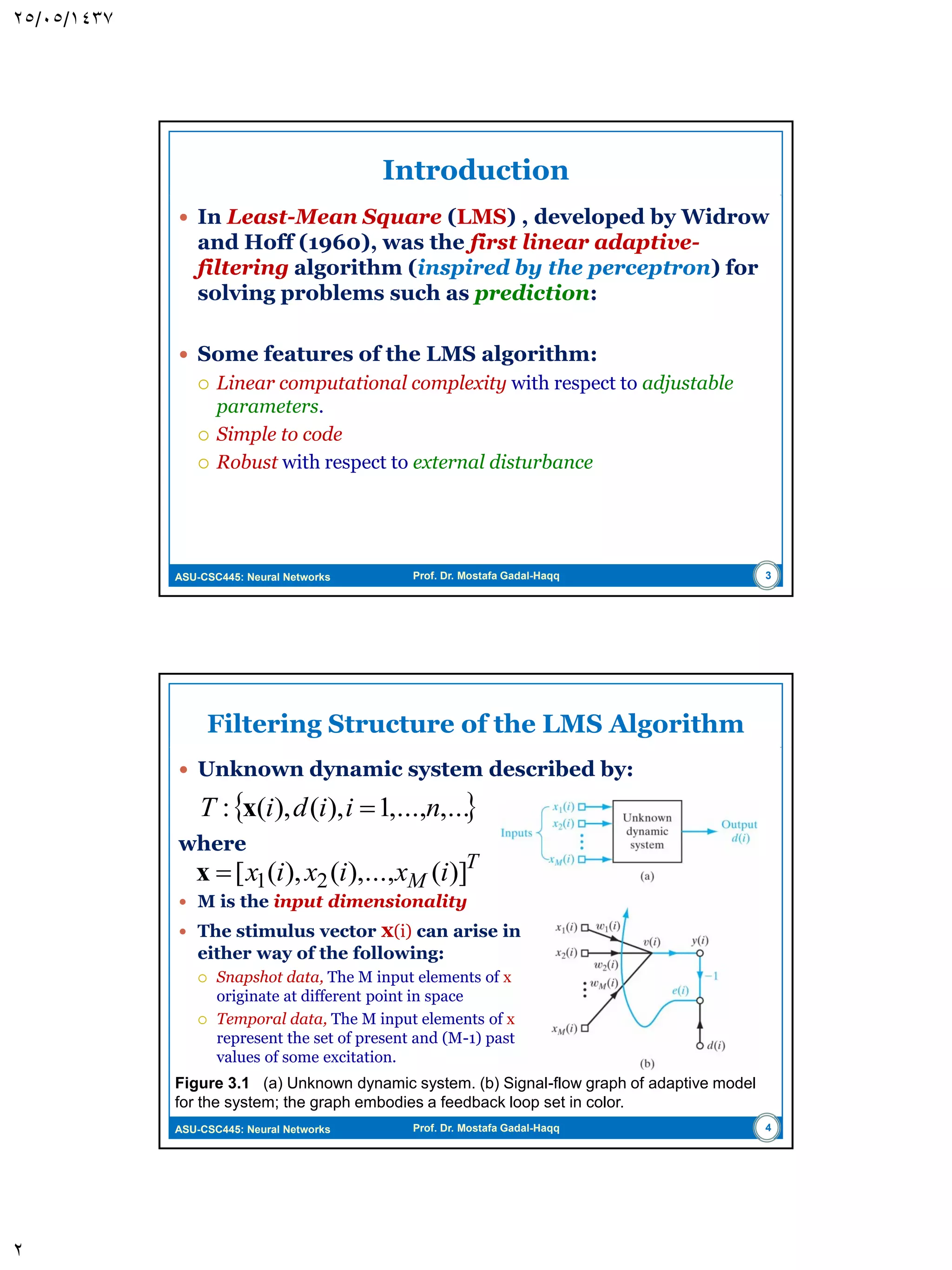
ASU-CSC445: Neural Networks Prof. Dr. Mostafa Gadal-Haqq  Introduction  Filtering Structure of the LMS Algorithm  Unconstrained Optimization: A Review  Method of Steepest Descent  Newton’s Method  Gauss-Newton Method  The Least-Mean Square Algorithm  Computer Experiment 2 Model Building Through Regression
ASU-CSC445: Neural Networks Prof. Dr. Mostafa Gadal-Haqq Introduction  In Least-Mean Square (LMS) , developed by Widrow and Hoff (1960), was the first linear adaptive- filtering algorithm (inspired by the perceptron) for solving problems such as prediction:  Some features of the LMS algorithm:  Linear computational complexity with respect to adjustable parameters.  Simple to code  Robust with respect to external disturbance 3
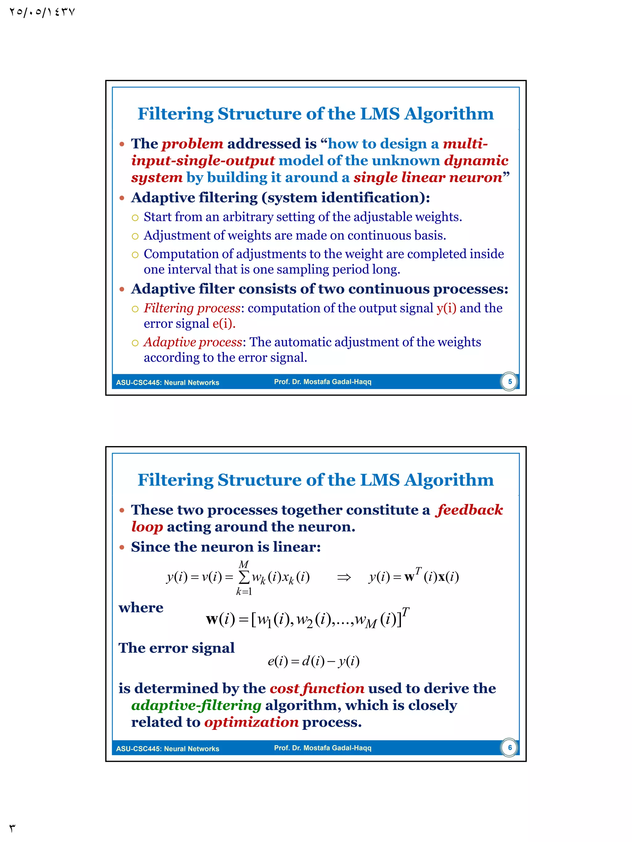
ASU-CSC445: Neural Networks Prof. Dr. Mostafa Gadal-Haqq Filtering Structure of the LMS Algorithm  Unknown dynamic system described by: Figure 3.1 (a) Unknown dynamic system. (b) Signal-flow graph of adaptive model for the system; the graph embodies a feedback loop set in color. 4 T M ixixix )](),...,(),([ 21x  ,...,...,1),(),(: niidiΤ x where  M is the input dimensionality  The stimulus vector x(i) can arise in either way of the following:  Snapshot data, The M input elements of x originate at different point in space  Temporal data, The M input elements of x represent the set of present and (M-1) past values of some excitation.
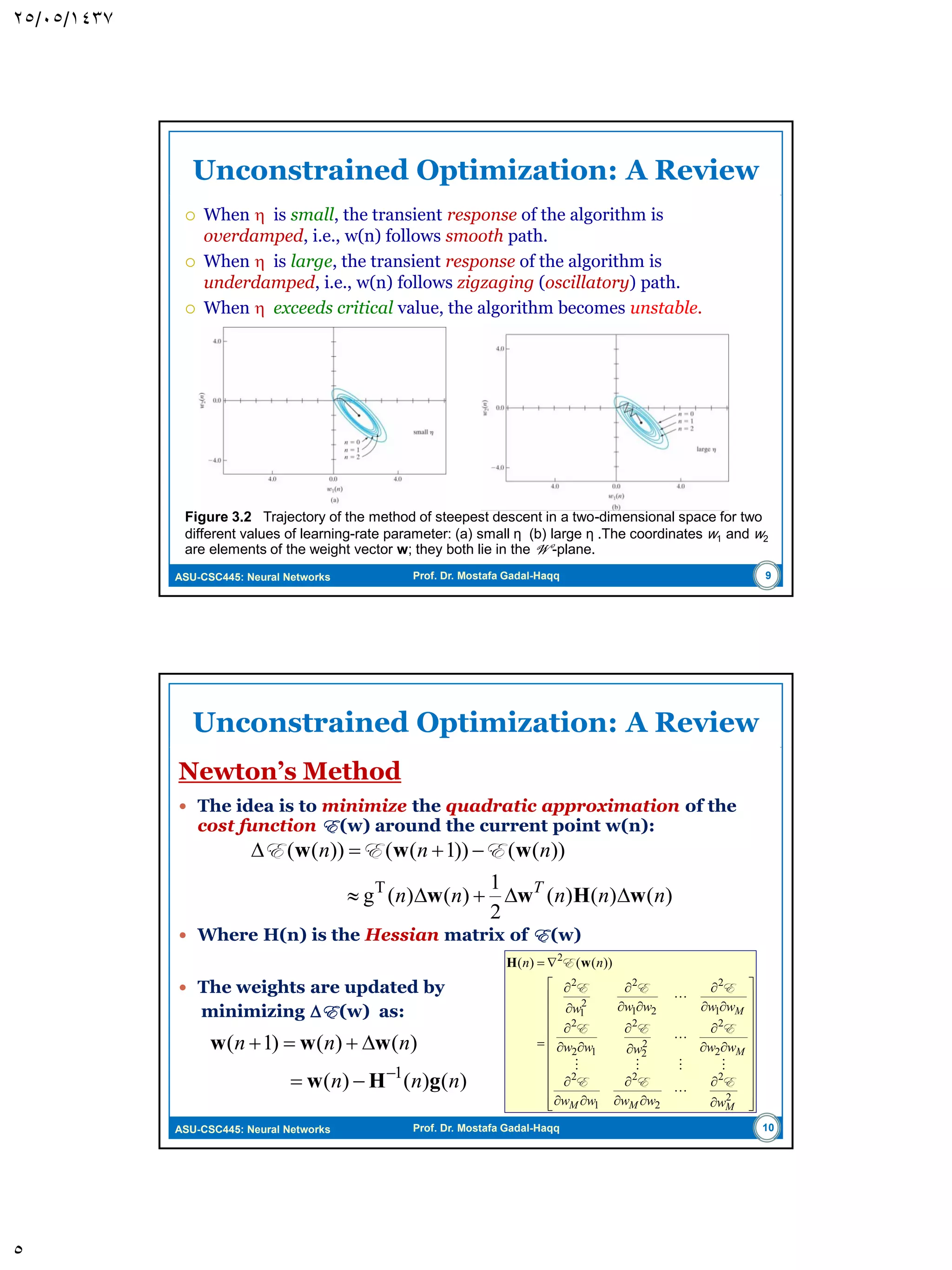
ASU-CSC445: Neural Networks Prof. Dr. Mostafa Gadal-Haqq Filtering Structure of the LMS Algorithm  The problem addressed is “how to design a multi- input-single-output model of the unknown dynamic system by building it around a single linear neuron”  Adaptive filtering (system identification):  Start from an arbitrary setting of the adjustable weights.  Adjustment of weights are made on continuous basis.  Computation of adjustments to the weight are completed inside one interval that is one sampling period long.  Adaptive filter consists of two continuous processes:  Filtering process: computation of the output signal y(i) and the error signal e(i).  Adaptive process: The automatic adjustment of the weights according to the error signal. 5
ASU-CSC445: Neural Networks Prof. Dr. Mostafa Gadal-Haqq Filtering Structure of the LMS Algorithm  These two processes together constitute a feedback loop acting around the neuron.  Since the neuron is linear: where The error signal is determined by the cost function used to derive the adaptive-filtering algorithm, which is closely related to optimization process. 6 )()()()()()()( 1 iiiyixiwiviy T M k kk xw   T M iwiwiwi )](),...,(),([)( 21w )()()( iyidie 
ASU-CSC445: Neural Networks Prof. Dr. Mostafa Gadal-Haqq Unconstrained Optimization: A Review  Consider the cost function E (w) that is continuously differentiable function of unknown weights w. we need to find the optimal solution w* that satisfies:  That is, we need to solve the unconstrained-optimization problem stated as: “Minimize the cost function E (w) with respect to the weight vector w”  The necessary condition for optimality:  Usually the solution is based on the idea of local iterative descent: Starting with a guess w(0), generate a sequence of weight vectors w(1), w(2), …, such that: 7 )(*)( ww EE  0*)(  wE ))(())1(( nn ww EE 
ASU-CSC445: Neural Networks Prof. Dr. Mostafa Gadal-Haqq Unconstrained Optimization: A Review Method of Steepest descent  The successive adjustments applied to the weight vector w are in the direction of steepest descent; that is in a direction opposite to the gradient of E (w).  If g = E (w) , then the steepest descent algorithm is  Where  is a positive constant called the step size, or learning- rate, parameter. In each step, the algorithm applies the correction:  HW: Prove the convergence of this algorithm and show how it is influenced by the learning rate . (Sec. 3.3 of Haykin) 8 )()()1( nnn gww  )( )()1()( n nnn g www  
ASU-CSC445: Neural Networks Prof. Dr. Mostafa Gadal-Haqq Unconstrained Optimization: A Review  When  is small, the transient response of the algorithm is overdamped, i.e., w(n) follows smooth path.  When  is large, the transient response of the algorithm is underdamped, i.e., w(n) follows zigzaging (oscillatory) path.  When  exceeds critical value, the algorithm becomes unstable. Figure 3.2 Trajectory of the method of steepest descent in a two-dimensional space for two different values of learning-rate parameter: (a) small η (b) large η .The coordinates w1 and w2 are elements of the weight vector w; they both lie in the W -plane. 9
ASU-CSC445: Neural Networks Prof. Dr. Mostafa Gadal-Haqq Unconstrained Optimization: A Review Newton’s Method  The idea is to minimize the quadratic approximation of the cost function E (w) around the current point w(n):  Where H(n) is the Hessian matrix of E (w)  The weights are updated by minimizing E (w) as: 10 )()()( 2 1 )()(g ))(())1(())(( T nnnnn nnn T wHww www   EEE                                           2 2 2 2 1 2 2 2 2 2 2 12 2 1 2 21 2 2 1 2 2 ))(()( MMM M M wwwww wwwww wwwww nn EEE EEE EEE E     wH )()()( )()()1( 1 nnn nnn gHw www   
ASU-CSC445: Neural Networks Prof. Dr. Mostafa Gadal-Haqq Unconstrained Optimization: A Review Newton’s Method  Generally, Newton’s method converges quickly and does not exhibit the zigzagging behavior of the method of steepest- descent.  However, Newton’s method has two main disadvantages:  the Hessian matrix H(n) has to be a positive definite matrix for all n, which is not guaranteed by the algorithm.  This is solved by the modified Gauss-Newton method.  It has high computational complexity. 11
ASU-CSC445: Neural Networks Prof. Dr. Mostafa Gadal-Haqq The Least-Mean Square Algorithm  The aim of the LMS algorithm is to minimize the instantaneous value of the cost function E (w) :  Differentiation of E (w), with respect to w, yields :  As with the least-square filters, the LMS operates on linear neuron, we can write: and Finally 12 )( 2 1 )ˆ( 2 newE ww w      )( )( ˆ )ˆ( ne ne E )( ˆ e(n) )()(ˆ)()( nnnidne T x w xw     )()( ˆ )ˆ( )( nenn x w w g     E )()()(ˆ)()(ˆ)1(ˆ nennngnn xwww  
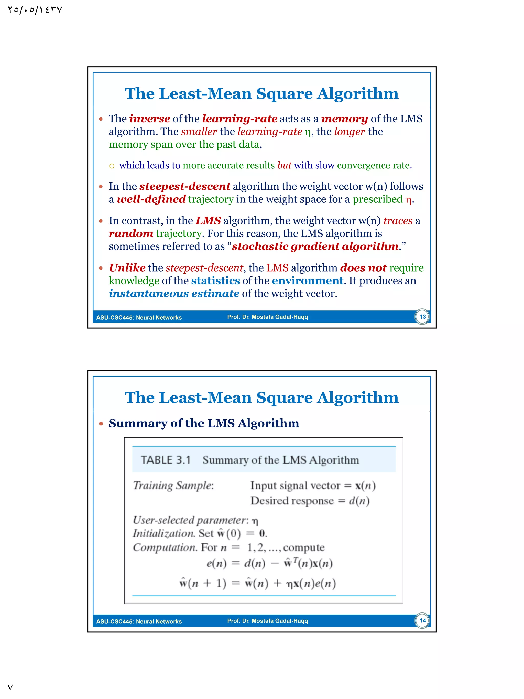
ASU-CSC445: Neural Networks Prof. Dr. Mostafa Gadal-Haqq The Least-Mean Square Algorithm  The inverse of the learning-rate acts as a memory of the LMS algorithm. The smaller the learning-rate , the longer the memory span over the past data,  which leads to more accurate results but with slow convergence rate.  In the steepest-descent algorithm the weight vector w(n) follows a well-defined trajectory in the weight space for a prescribed .  In contrast, in the LMS algorithm, the weight vector w(n) traces a random trajectory. For this reason, the LMS algorithm is sometimes referred to as “stochastic gradient algorithm.”  Unlike the steepest-descent, the LMS algorithm does not require knowledge of the statistics of the environment. It produces an instantaneous estimate of the weight vector. 13
ASU-CSC445: Neural Networks Prof. Dr. Mostafa Gadal-Haqq The Least-Mean Square Algorithm  Summary of the LMS Algorithm 14
ASU-CSC445: Neural Networks Prof. Dr. Mostafa Gadal-Haqq Virtues and Limitation of the LMS Alg. Computational Simplicity and Efficiency:  The Algorithm is very simple to code, only two or three line of code.  the computational complexity of the algorithm is linear in the adjustable parameters. 15
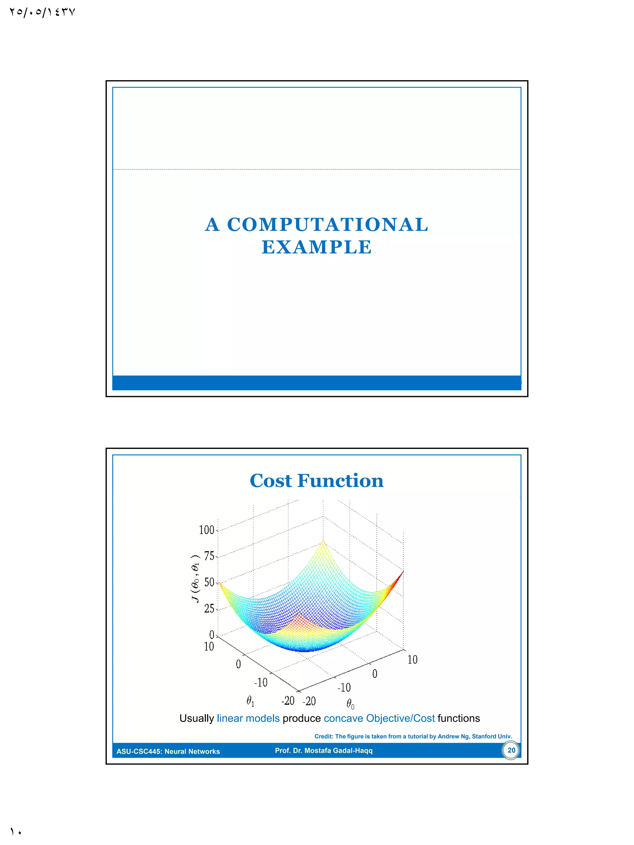
A COMPUTATIONAL EXAMPLE 16
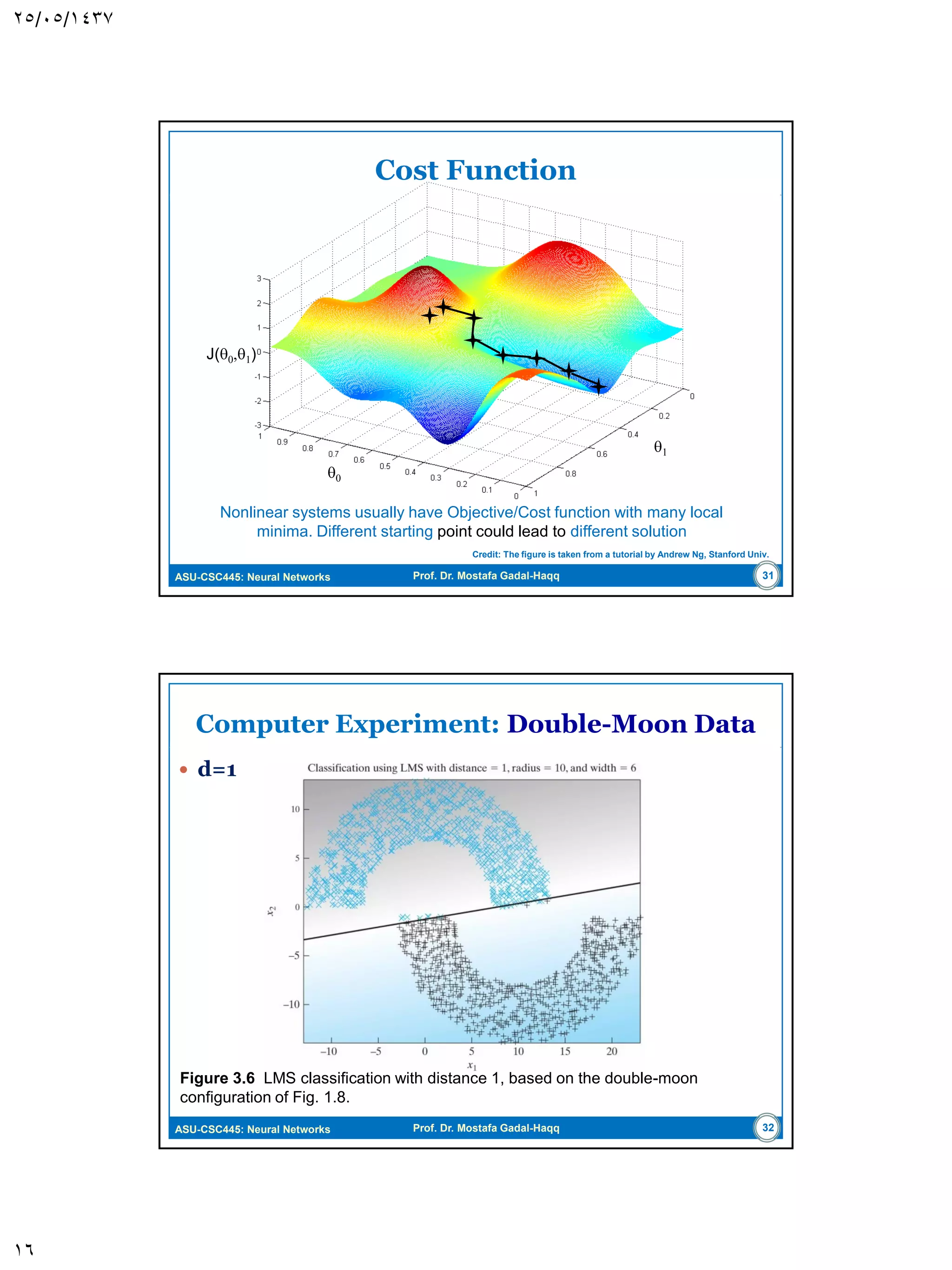
ASU-CSC445: Neural Networks Prof. Dr. Mostafa Gadal-Haqq Cost Function Usually linear models produce concave cost functions Figure copyright of Andrew Ng. 17
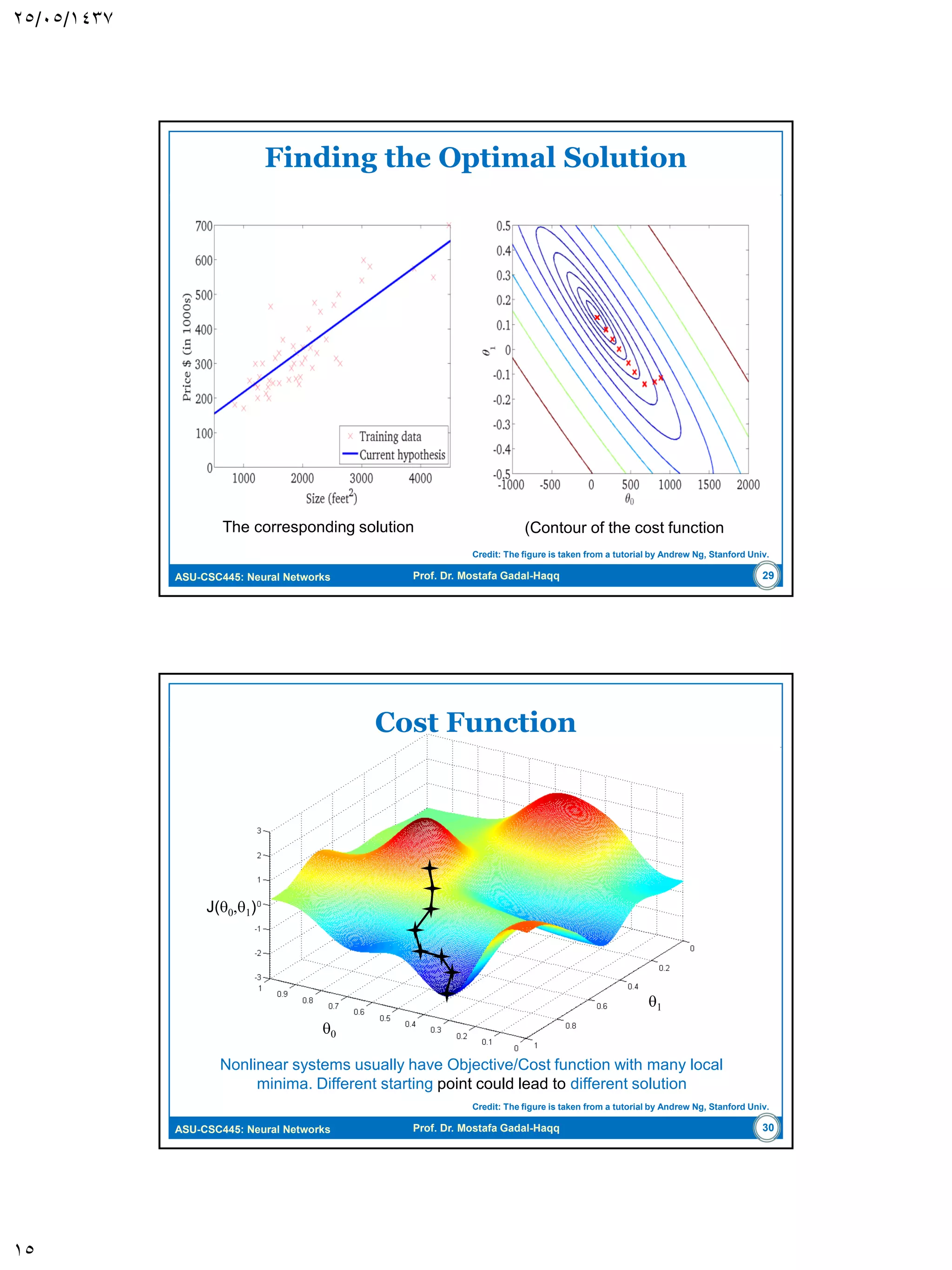
ASU-CSC445: Neural Networks Prof. Dr. Mostafa Gadal-Haqq 1 0 J(0,1) Cost Function Different starting point could lead to different solutionFigure copyright of Andrew Ng. 18
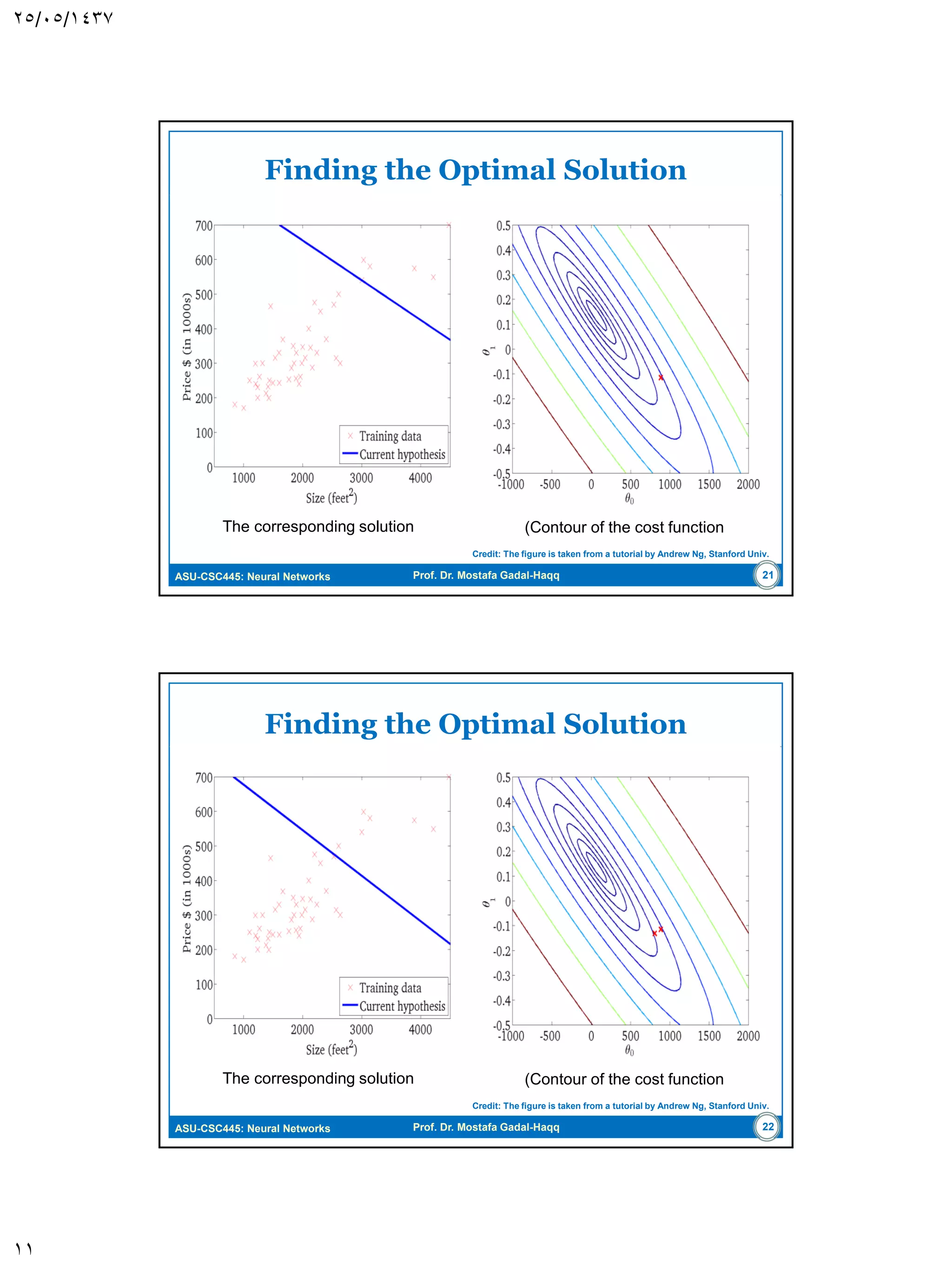
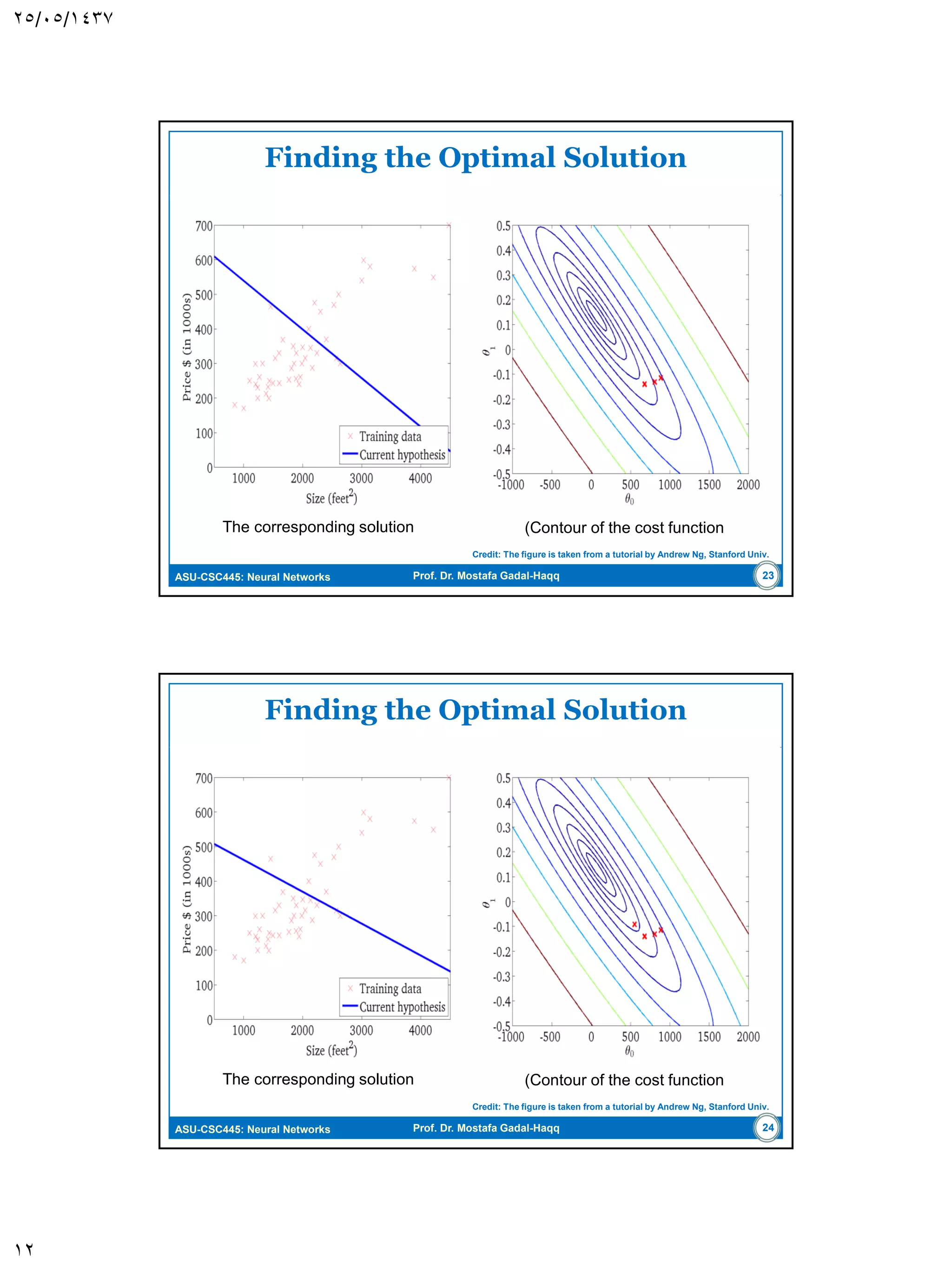
ASU-CSC445: Neural Networks Prof. Dr. Mostafa Gadal-Haqq The corresponding solution (Contour of the cost function Finding a Solution Figure copyright of Andrew Ng. 20
The corresponding solution (Contour of the cost function Figure copyright of Andrew Ng. 21
The corresponding solution (Contour of the cost function Figure copyright of Andrew Ng. 22
The corresponding solution (Contour of the cost function Figure copyright of Andrew Ng. 23
The corresponding solution (Contour of the cost function Figure copyright of Andrew Ng. 24
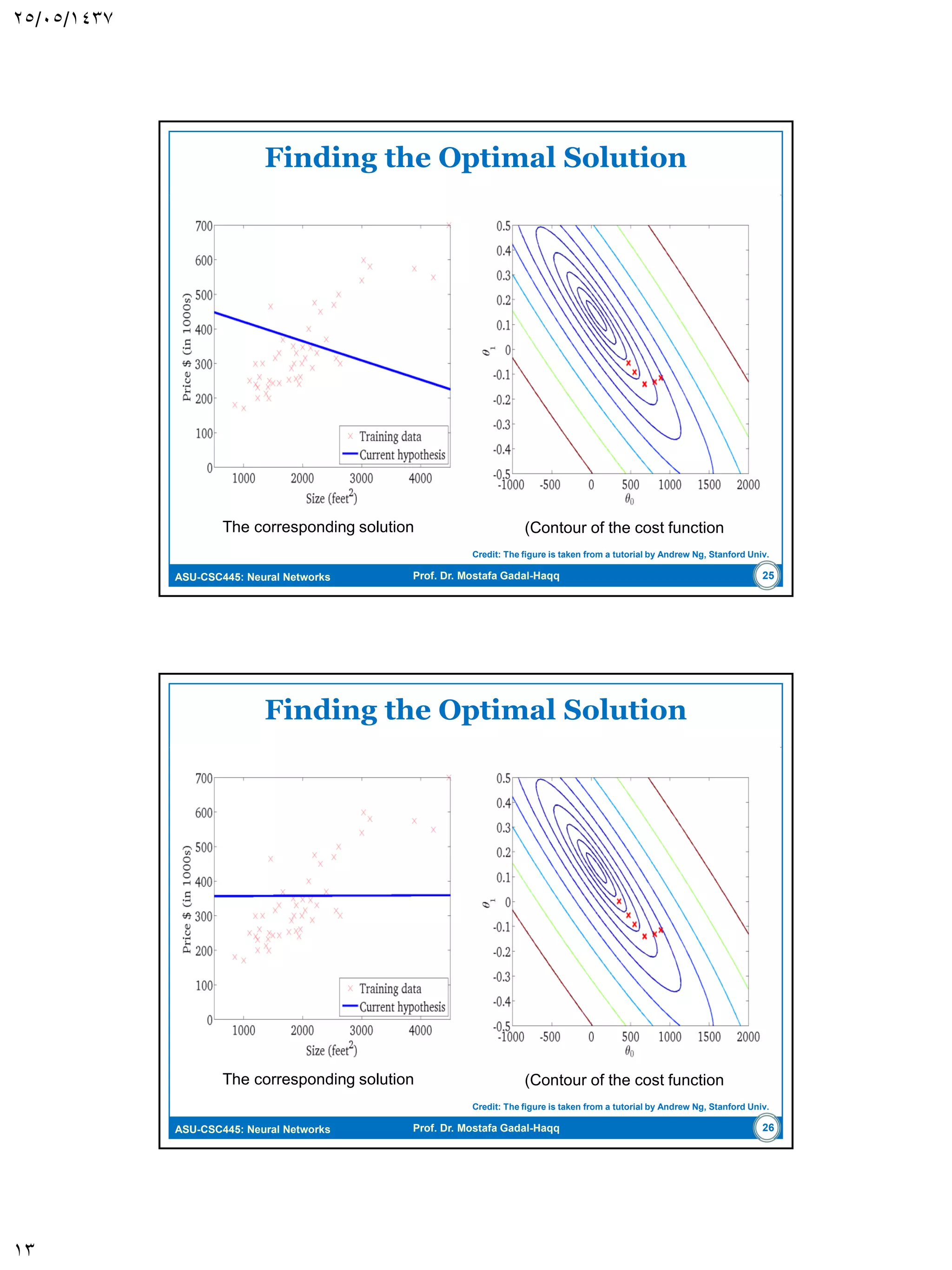
The corresponding solution (Contour of the cost function Figure copyright of Andrew Ng. 25
The corresponding solution (Contour of the cost function Figure copyright of Andrew Ng. 26
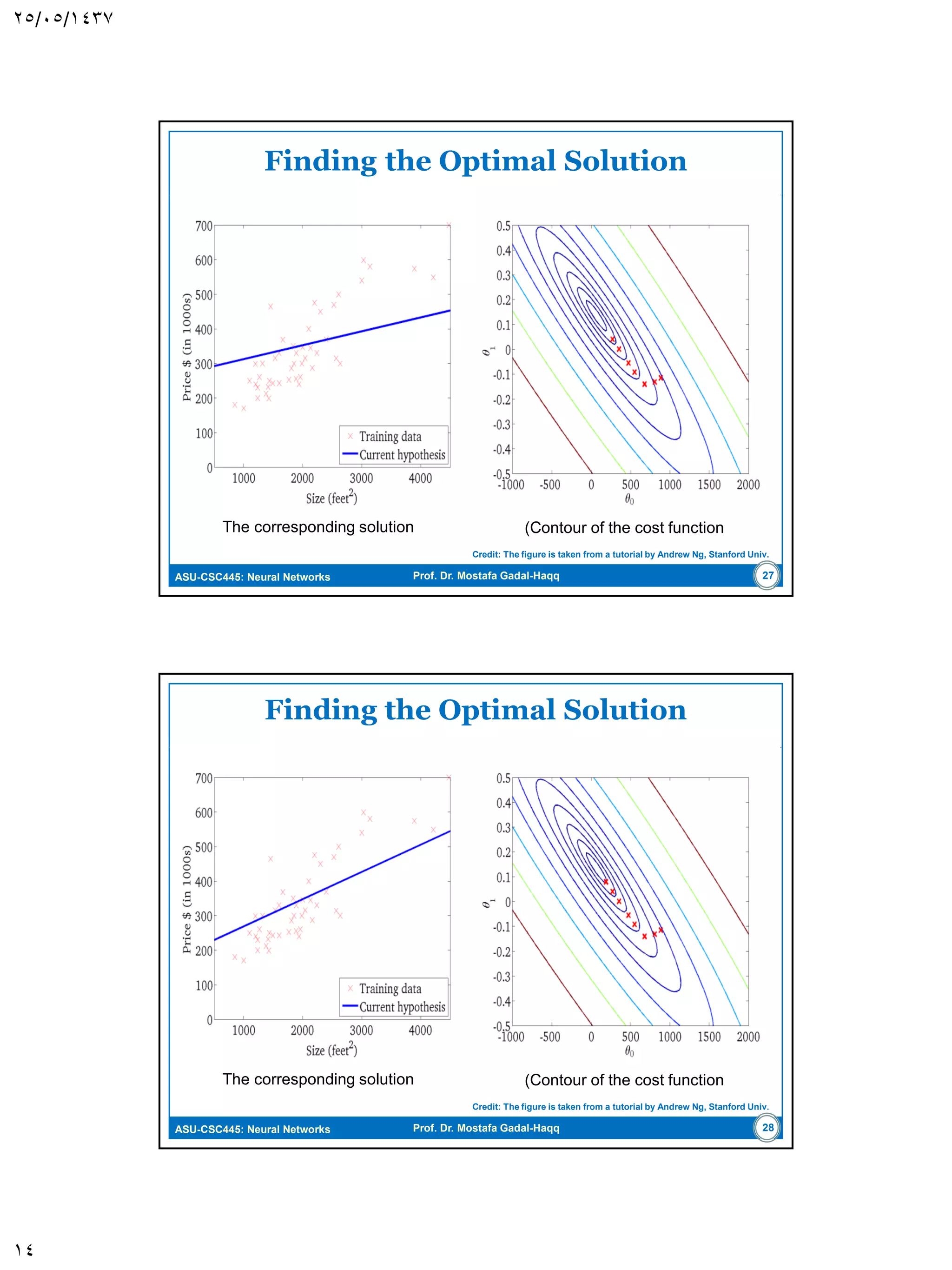
The corresponding solution (Contour of the cost function Figure copyright of Andrew Ng. 27
The corresponding solution (Contour of the cost function Figure copyright of Andrew Ng. 28
ASU-CSC445: Neural Networks Prof. Dr. Mostafa Gadal-Haqq Virtues and Limitation of the LMS Alg. Robustness  Since the LMS is model independent, therefore it is robust with respect to disturbance.  That is, the LMS is optimal in accordance with H norm (the response of the transfer function T of the estimator).  The philosophy of the optimality is to accommodate with the worst-case scenario: • “If you don’t know what you are up against, plan for the worst scenario and optimize.” Figure 3.8 Formulation of the optimal H∞ estimation problem. The generic estimation error at the transfer operator’s output could be the weight-error vector, the explanational error, etc. 29
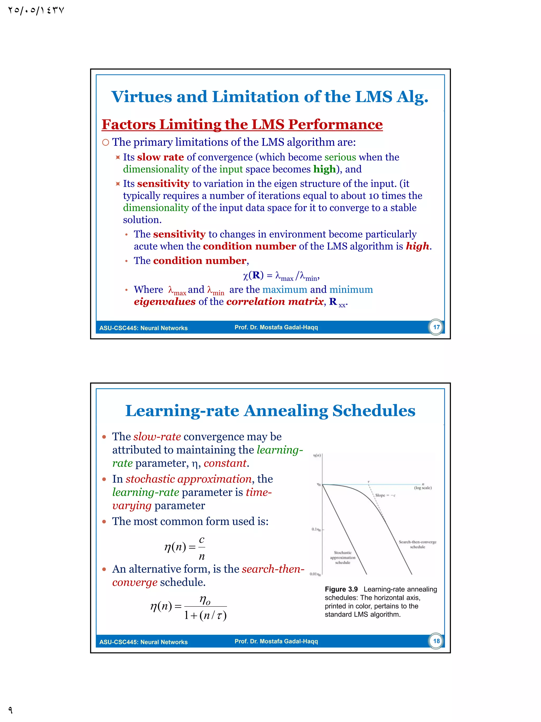
ASU-CSC445: Neural Networks Prof. Dr. Mostafa Gadal-Haqq Virtues and Limitation of the LMS Alg. Factors Limiting the LMS Performance  The primary limitations of the LMS algorithm are:  Its slow rate of convergence (which become serious when the dimensionality of the input space becomes high), and  Its sensitivity to variation in the eigen structure of the input. (it typically requires a number of iterations equal to about 10 times the dimensionality of the input data space for it to converge to a stable solution. • The sensitivity to changes in environment become particularly acute when the condition number of the LMS algorithm is high. • The condition number, (R) = max /min, • Where max and min are the maximum and minimum eigenvalues of the correlation matrix, R xx. 30
ASU-CSC445: Neural Networks Prof. Dr. Mostafa Gadal-Haqq Learning-rate Annealing Schedules  The slow-rate convergence may be attributed to maintaining the learning- rate parameter, , constant.  In stochastic approximation, the learning-rate parameter is time- varying parameter  The most common form used is:  An alternative form, is the search-then- converge schedule. Figure 3.9 Learning-rate annealing schedules: The horizontal axis, printed in color, pertains to the standard LMS algorithm. 31 n c n )( )/(1 )(    n n o  
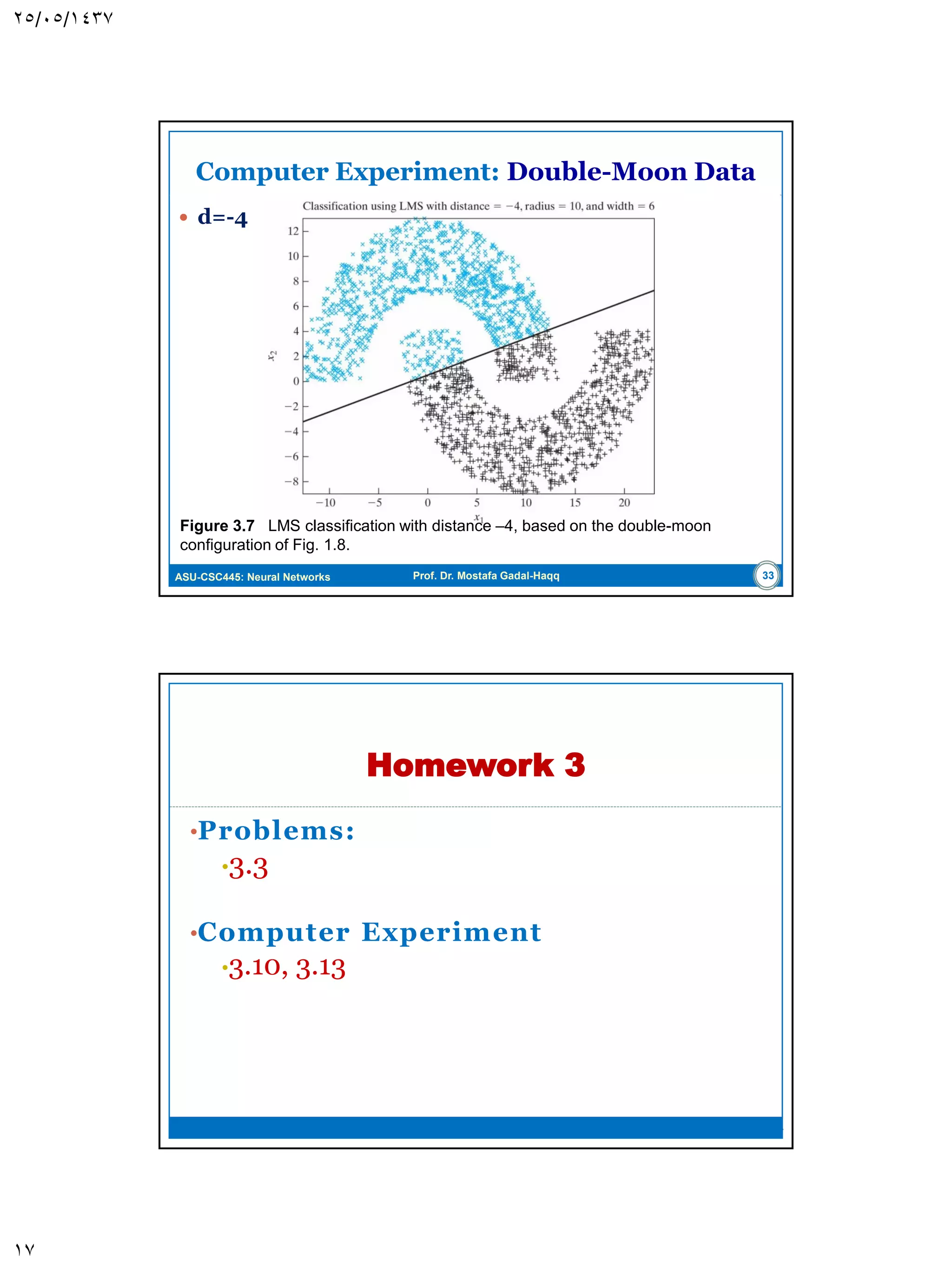
ASU-CSC445: Neural Networks Prof. Dr. Mostafa Gadal-Haqq Computer Experiment  d=1 Figure 3.6 LMS classification with distance 1, based on the double-moon configuration of Fig. 1.8. 32
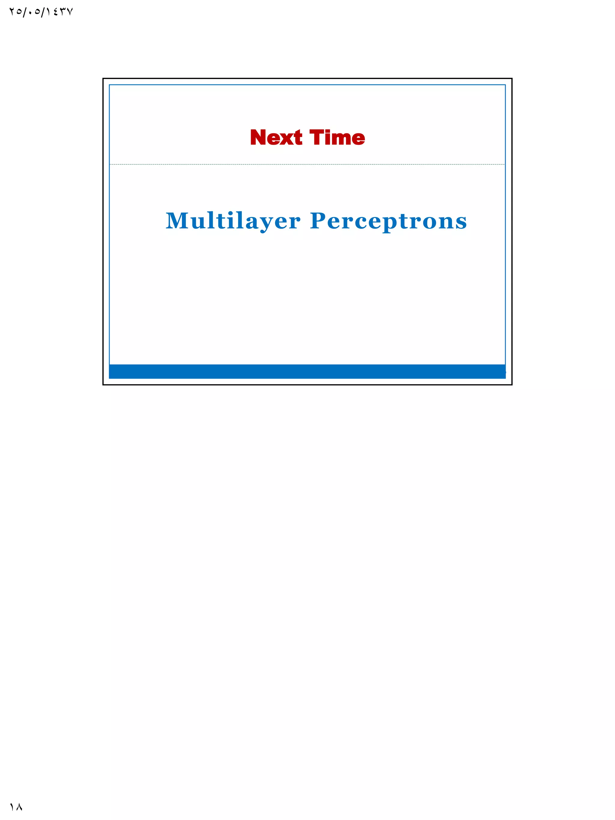
ASU-CSC445: Neural Networks Prof. Dr. Mostafa Gadal-Haqq Computer Experiment  d=-4 Figure 3.7 LMS classification with distance –4, based on the double-moon configuration of Fig. 1.8. 33
•Problems: •3.3 •Computer Experiment •3.10, 3.13 Homework 3 34
Multilayer Perceptrons Next Time 35

Neural Networks: Least Mean Square (LSM) Algorithm

  • 1.
    CHAPTER 03 THE LEAST-MEANSQUARE ALGORITHM CSC445: Neural Networks Prof. Dr. Mostafa Gadal-Haqq M. Mostafa Computer Science Department Faculty of Computer & Information Sciences AIN SHAMS UNIVERSITY (most of figures in this presentation are copyrighted to Pearson Education, Inc.)
  • 2.
    ASU-CSC445: Neural NetworksProf. Dr. Mostafa Gadal-Haqq  Introduction  Filtering Structure of the LMS Algorithm  Unconstrained Optimization: A Review  Method of Steepest Descent  Newton’s Method  Gauss-Newton Method  The Least-Mean Square Algorithm  Computer Experiment 2 Model Building Through Regression
  • 3.
    ASU-CSC445: Neural NetworksProf. Dr. Mostafa Gadal-Haqq Introduction  In Least-Mean Square (LMS) , developed by Widrow and Hoff (1960), was the first linear adaptive- filtering algorithm (inspired by the perceptron) for solving problems such as prediction:  Some features of the LMS algorithm:  Linear computational complexity with respect to adjustable parameters.  Simple to code  Robust with respect to external disturbance 3
  • 4.
    ASU-CSC445: Neural NetworksProf. Dr. Mostafa Gadal-Haqq Filtering Structure of the LMS Algorithm  Unknown dynamic system described by: Figure 3.1 (a) Unknown dynamic system. (b) Signal-flow graph of adaptive model for the system; the graph embodies a feedback loop set in color. 4 T M ixixix )](),...,(),([ 21x  ,...,...,1),(),(: niidiΤ x where  M is the input dimensionality  The stimulus vector x(i) can arise in either way of the following:  Snapshot data, The M input elements of x originate at different point in space  Temporal data, The M input elements of x represent the set of present and (M-1) past values of some excitation.
  • 5.
    ASU-CSC445: Neural NetworksProf. Dr. Mostafa Gadal-Haqq Filtering Structure of the LMS Algorithm  The problem addressed is “how to design a multi- input-single-output model of the unknown dynamic system by building it around a single linear neuron”  Adaptive filtering (system identification):  Start from an arbitrary setting of the adjustable weights.  Adjustment of weights are made on continuous basis.  Computation of adjustments to the weight are completed inside one interval that is one sampling period long.  Adaptive filter consists of two continuous processes:  Filtering process: computation of the output signal y(i) and the error signal e(i).  Adaptive process: The automatic adjustment of the weights according to the error signal. 5
  • 6.
    ASU-CSC445: Neural NetworksProf. Dr. Mostafa Gadal-Haqq Filtering Structure of the LMS Algorithm  These two processes together constitute a feedback loop acting around the neuron.  Since the neuron is linear: where The error signal is determined by the cost function used to derive the adaptive-filtering algorithm, which is closely related to optimization process. 6 )()()()()()()( 1 iiiyixiwiviy T M k kk xw   T M iwiwiwi )](),...,(),([)( 21w )()()( iyidie 
  • 7.
    ASU-CSC445: Neural NetworksProf. Dr. Mostafa Gadal-Haqq Unconstrained Optimization: A Review  Consider the cost function E (w) that is continuously differentiable function of unknown weights w. we need to find the optimal solution w* that satisfies:  That is, we need to solve the unconstrained-optimization problem stated as: “Minimize the cost function E (w) with respect to the weight vector w”  The necessary condition for optimality:  Usually the solution is based on the idea of local iterative descent: Starting with a guess w(0), generate a sequence of weight vectors w(1), w(2), …, such that: 7 )(*)( ww EE  0*)(  wE ))(())1(( nn ww EE 
  • 8.
    ASU-CSC445: Neural NetworksProf. Dr. Mostafa Gadal-Haqq Unconstrained Optimization: A Review Method of Steepest descent  The successive adjustments applied to the weight vector w are in the direction of steepest descent; that is in a direction opposite to the gradient of E (w).  If g = E (w) , then the steepest descent algorithm is  Where  is a positive constant called the step size, or learning- rate, parameter. In each step, the algorithm applies the correction:  HW: Prove the convergence of this algorithm and show how it is influenced by the learning rate . (Sec. 3.3 of Haykin) 8 )()()1( nnn gww  )( )()1()( n nnn g www  
  • 9.
    ASU-CSC445: Neural NetworksProf. Dr. Mostafa Gadal-Haqq Unconstrained Optimization: A Review  When  is small, the transient response of the algorithm is overdamped, i.e., w(n) follows smooth path.  When  is large, the transient response of the algorithm is underdamped, i.e., w(n) follows zigzaging (oscillatory) path.  When  exceeds critical value, the algorithm becomes unstable. Figure 3.2 Trajectory of the method of steepest descent in a two-dimensional space for two different values of learning-rate parameter: (a) small η (b) large η .The coordinates w1 and w2 are elements of the weight vector w; they both lie in the W -plane. 9
  • 10.
    ASU-CSC445: Neural NetworksProf. Dr. Mostafa Gadal-Haqq Unconstrained Optimization: A Review Newton’s Method  The idea is to minimize the quadratic approximation of the cost function E (w) around the current point w(n):  Where H(n) is the Hessian matrix of E (w)  The weights are updated by minimizing E (w) as: 10 )()()( 2 1 )()(g ))(())1(())(( T nnnnn nnn T wHww www   EEE                                           2 2 2 2 1 2 2 2 2 2 2 12 2 1 2 21 2 2 1 2 2 ))(()( MMM M M wwwww wwwww wwwww nn EEE EEE EEE E     wH )()()( )()()1( 1 nnn nnn gHw www   
  • 11.
    ASU-CSC445: Neural NetworksProf. Dr. Mostafa Gadal-Haqq Unconstrained Optimization: A Review Newton’s Method  Generally, Newton’s method converges quickly and does not exhibit the zigzagging behavior of the method of steepest- descent.  However, Newton’s method has two main disadvantages:  the Hessian matrix H(n) has to be a positive definite matrix for all n, which is not guaranteed by the algorithm.  This is solved by the modified Gauss-Newton method.  It has high computational complexity. 11
  • 12.
    ASU-CSC445: Neural NetworksProf. Dr. Mostafa Gadal-Haqq The Least-Mean Square Algorithm  The aim of the LMS algorithm is to minimize the instantaneous value of the cost function E (w) :  Differentiation of E (w), with respect to w, yields :  As with the least-square filters, the LMS operates on linear neuron, we can write: and Finally 12 )( 2 1 )ˆ( 2 newE ww w      )( )( ˆ )ˆ( ne ne E )( ˆ e(n) )()(ˆ)()( nnnidne T x w xw     )()( ˆ )ˆ( )( nenn x w w g     E )()()(ˆ)()(ˆ)1(ˆ nennngnn xwww  
  • 13.
    ASU-CSC445: Neural NetworksProf. Dr. Mostafa Gadal-Haqq The Least-Mean Square Algorithm  The inverse of the learning-rate acts as a memory of the LMS algorithm. The smaller the learning-rate , the longer the memory span over the past data,  which leads to more accurate results but with slow convergence rate.  In the steepest-descent algorithm the weight vector w(n) follows a well-defined trajectory in the weight space for a prescribed .  In contrast, in the LMS algorithm, the weight vector w(n) traces a random trajectory. For this reason, the LMS algorithm is sometimes referred to as “stochastic gradient algorithm.”  Unlike the steepest-descent, the LMS algorithm does not require knowledge of the statistics of the environment. It produces an instantaneous estimate of the weight vector. 13
  • 14.
    ASU-CSC445: Neural NetworksProf. Dr. Mostafa Gadal-Haqq The Least-Mean Square Algorithm  Summary of the LMS Algorithm 14
  • 15.
    ASU-CSC445: Neural NetworksProf. Dr. Mostafa Gadal-Haqq Virtues and Limitation of the LMS Alg. Computational Simplicity and Efficiency:  The Algorithm is very simple to code, only two or three line of code.  the computational complexity of the algorithm is linear in the adjustable parameters. 15
  • 16.
  • 17.
    ASU-CSC445: Neural NetworksProf. Dr. Mostafa Gadal-Haqq Cost Function Usually linear models produce concave cost functions Figure copyright of Andrew Ng. 17
  • 18.
    ASU-CSC445: Neural NetworksProf. Dr. Mostafa Gadal-Haqq 1 0 J(0,1) Cost Function Different starting point could lead to different solutionFigure copyright of Andrew Ng. 18
  • 19.
    ASU-CSC445: Neural NetworksProf. Dr. Mostafa Gadal-Haqq The corresponding solution (Contour of the cost function Finding a Solution Figure copyright of Andrew Ng. 20
  • 20.
    The corresponding solution(Contour of the cost function Figure copyright of Andrew Ng. 21
  • 21.
    The corresponding solution(Contour of the cost function Figure copyright of Andrew Ng. 22
  • 22.
    The corresponding solution(Contour of the cost function Figure copyright of Andrew Ng. 23
  • 23.
    The corresponding solution(Contour of the cost function Figure copyright of Andrew Ng. 24
  • 24.
    The corresponding solution(Contour of the cost function Figure copyright of Andrew Ng. 25
  • 25.
    The corresponding solution(Contour of the cost function Figure copyright of Andrew Ng. 26
  • 26.
    The corresponding solution(Contour of the cost function Figure copyright of Andrew Ng. 27
  • 27.
    The corresponding solution(Contour of the cost function Figure copyright of Andrew Ng. 28
  • 28.
    ASU-CSC445: Neural NetworksProf. Dr. Mostafa Gadal-Haqq Virtues and Limitation of the LMS Alg. Robustness  Since the LMS is model independent, therefore it is robust with respect to disturbance.  That is, the LMS is optimal in accordance with H norm (the response of the transfer function T of the estimator).  The philosophy of the optimality is to accommodate with the worst-case scenario: • “If you don’t know what you are up against, plan for the worst scenario and optimize.” Figure 3.8 Formulation of the optimal H∞ estimation problem. The generic estimation error at the transfer operator’s output could be the weight-error vector, the explanational error, etc. 29
  • 29.
    ASU-CSC445: Neural NetworksProf. Dr. Mostafa Gadal-Haqq Virtues and Limitation of the LMS Alg. Factors Limiting the LMS Performance  The primary limitations of the LMS algorithm are:  Its slow rate of convergence (which become serious when the dimensionality of the input space becomes high), and  Its sensitivity to variation in the eigen structure of the input. (it typically requires a number of iterations equal to about 10 times the dimensionality of the input data space for it to converge to a stable solution. • The sensitivity to changes in environment become particularly acute when the condition number of the LMS algorithm is high. • The condition number, (R) = max /min, • Where max and min are the maximum and minimum eigenvalues of the correlation matrix, R xx. 30
  • 30.
    ASU-CSC445: Neural NetworksProf. Dr. Mostafa Gadal-Haqq Learning-rate Annealing Schedules  The slow-rate convergence may be attributed to maintaining the learning- rate parameter, , constant.  In stochastic approximation, the learning-rate parameter is time- varying parameter  The most common form used is:  An alternative form, is the search-then- converge schedule. Figure 3.9 Learning-rate annealing schedules: The horizontal axis, printed in color, pertains to the standard LMS algorithm. 31 n c n )( )/(1 )(    n n o  
  • 31.
    ASU-CSC445: Neural NetworksProf. Dr. Mostafa Gadal-Haqq Computer Experiment  d=1 Figure 3.6 LMS classification with distance 1, based on the double-moon configuration of Fig. 1.8. 32
  • 32.
    ASU-CSC445: Neural NetworksProf. Dr. Mostafa Gadal-Haqq Computer Experiment  d=-4 Figure 3.7 LMS classification with distance –4, based on the double-moon configuration of Fig. 1.8. 33
  • 33.
  • 34.