Download as PDF, PPTX


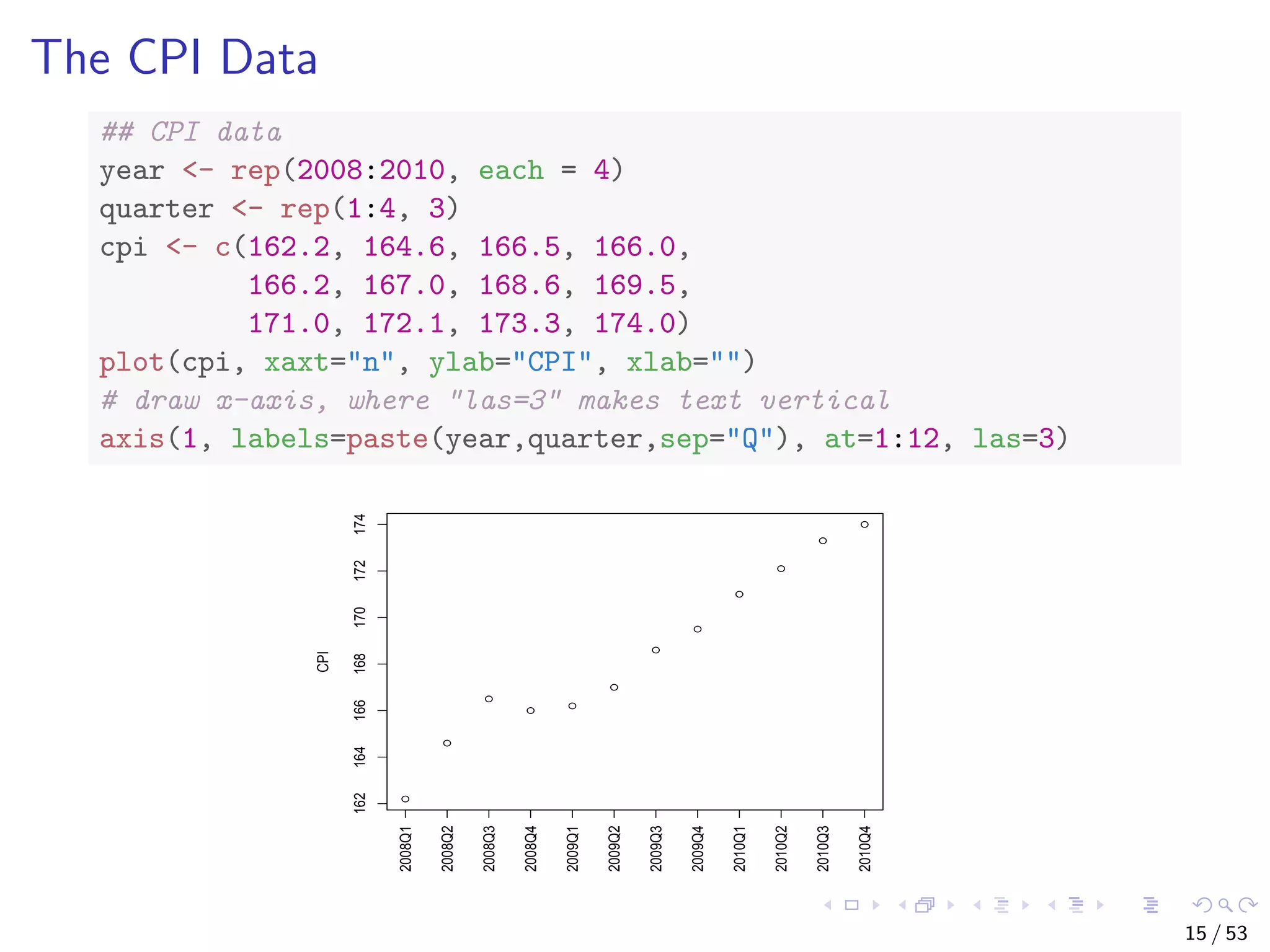
![Linear Regression ## correlation between CPI and year / quarter cor(year, cpi) ## [1] 0.9096316 cor(quarter, cpi) ## [1] 0.3738028 ## build a linear regression model with function lm() fit <- lm(cpi ~ year + quarter) fit ## ## Call: ## lm(formula = cpi ~ year + quarter) ## ## Coefficients: ## (Intercept) year quarter ## -7644.488 3.888 1.167 16 / 53](https://image.slidesharecdn.com/rdm-slides-regression-classification-190703041150/75/RDataMining-slides-regression-classification-16-2048.jpg)
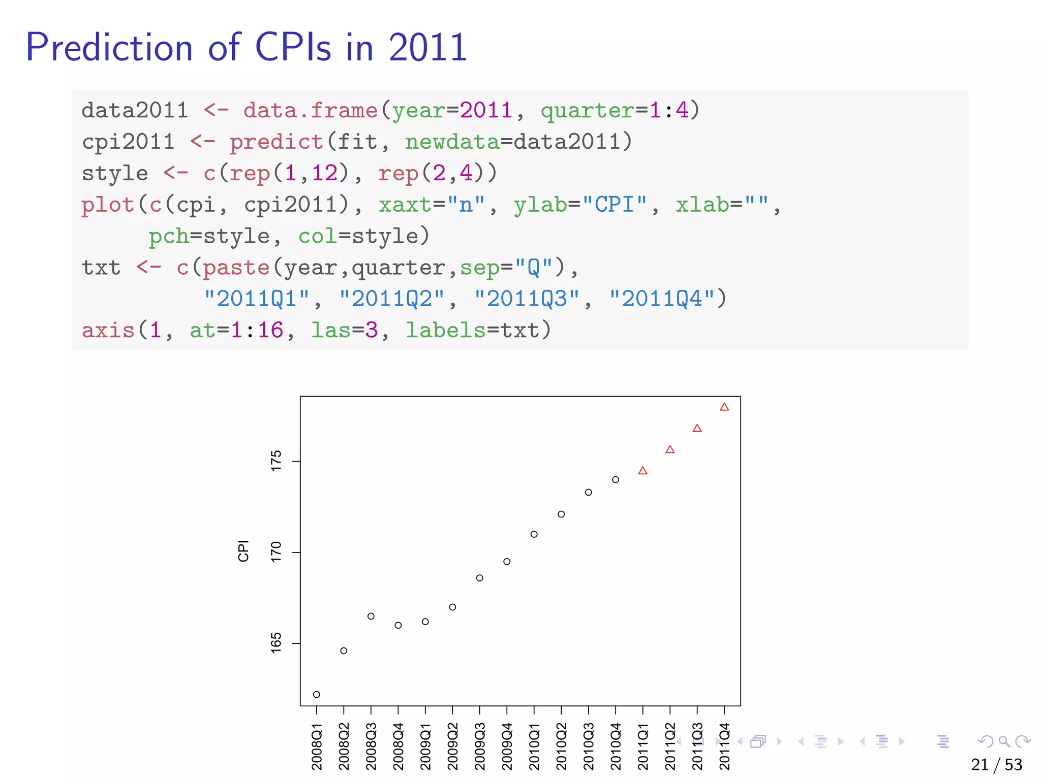
![With the above linear model, CPI is calculated as cpi = c0 + c1 ∗ year + c2 ∗ quarter, where c0, c1 and c2 are coefficients from model fit. What will the CPI be in 2011? # make prediction cpi2011 <- fit$coefficients[[1]] + fit$coefficients[[2]] * 2011 + fit$coefficients[[3]] * (1:4) cpi2011 ## [1] 174.4417 175.6083 176.7750 177.9417 17 / 53](https://image.slidesharecdn.com/rdm-slides-regression-classification-190703041150/75/RDataMining-slides-regression-classification-17-2048.jpg)
![With the above linear model, CPI is calculated as cpi = c0 + c1 ∗ year + c2 ∗ quarter, where c0, c1 and c2 are coefficients from model fit. What will the CPI be in 2011? # make prediction cpi2011 <- fit$coefficients[[1]] + fit$coefficients[[2]] * 2011 + fit$coefficients[[3]] * (1:4) cpi2011 ## [1] 174.4417 175.6083 176.7750 177.9417 An easier way is to use function predict(). 17 / 53](https://image.slidesharecdn.com/rdm-slides-regression-classification-190703041150/75/RDataMining-slides-regression-classification-18-2048.jpg)
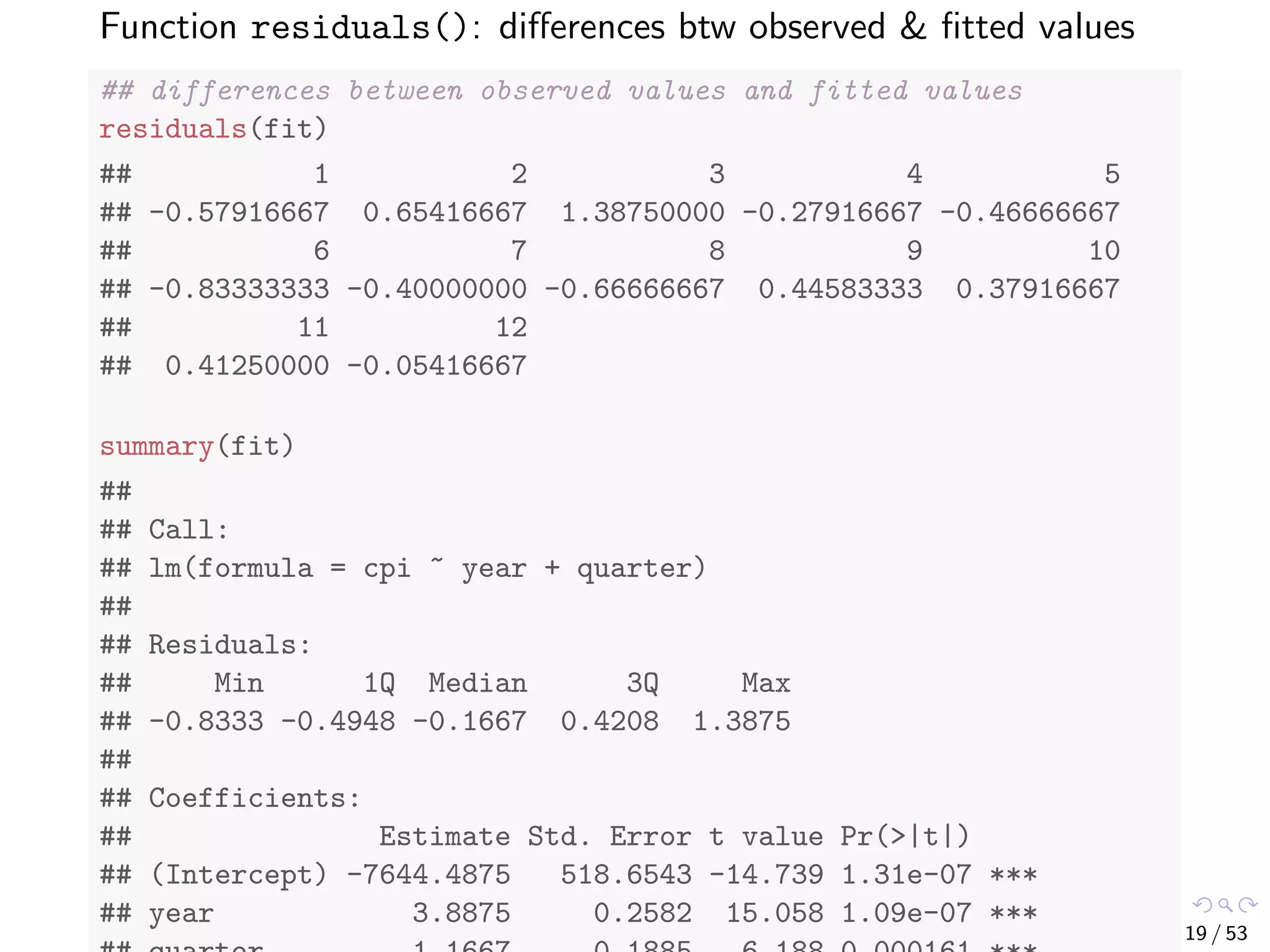
![More details of the model can be obtained with the code below. ## attributes of the model attributes(fit) ## $names ## [1] "coefficients" "residuals" "effects" ## [4] "rank" "fitted.values" "assign" ## [7] "qr" "df.residual" "xlevels" ## [10] "call" "terms" "model" ## ## $class ## [1] "lm" fit$coefficients ## (Intercept) year quarter ## -7644.487500 3.887500 1.166667 18 / 53](https://image.slidesharecdn.com/rdm-slides-regression-classification-190703041150/75/RDataMining-slides-regression-classification-19-2048.jpg)
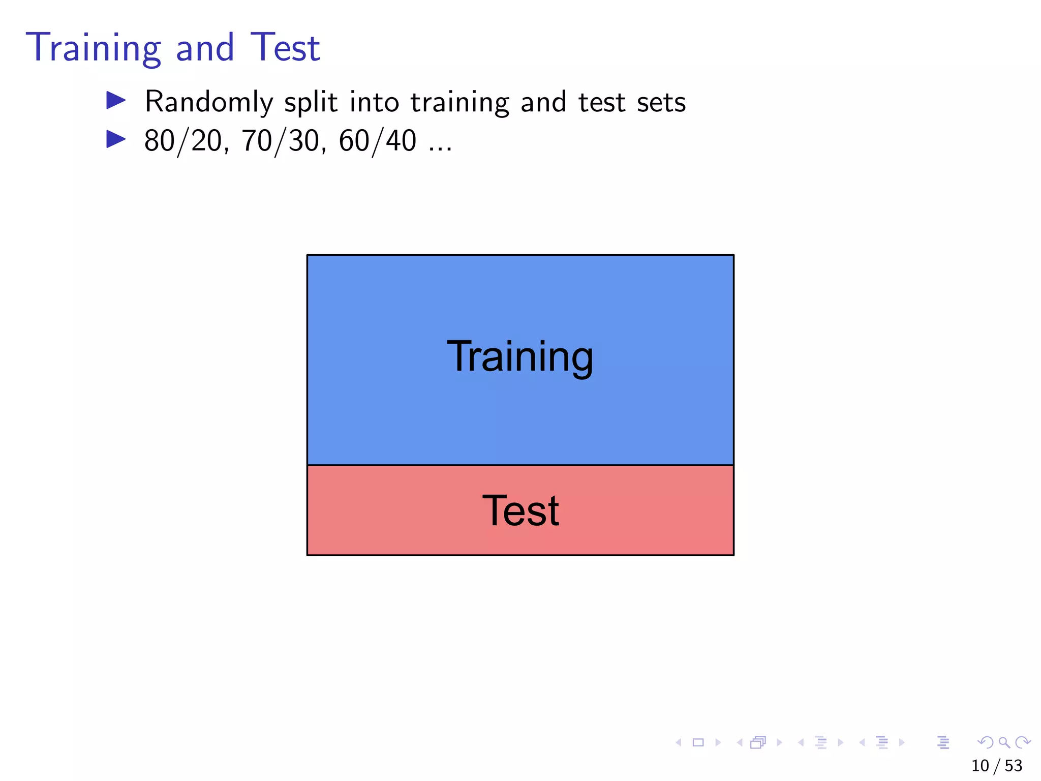
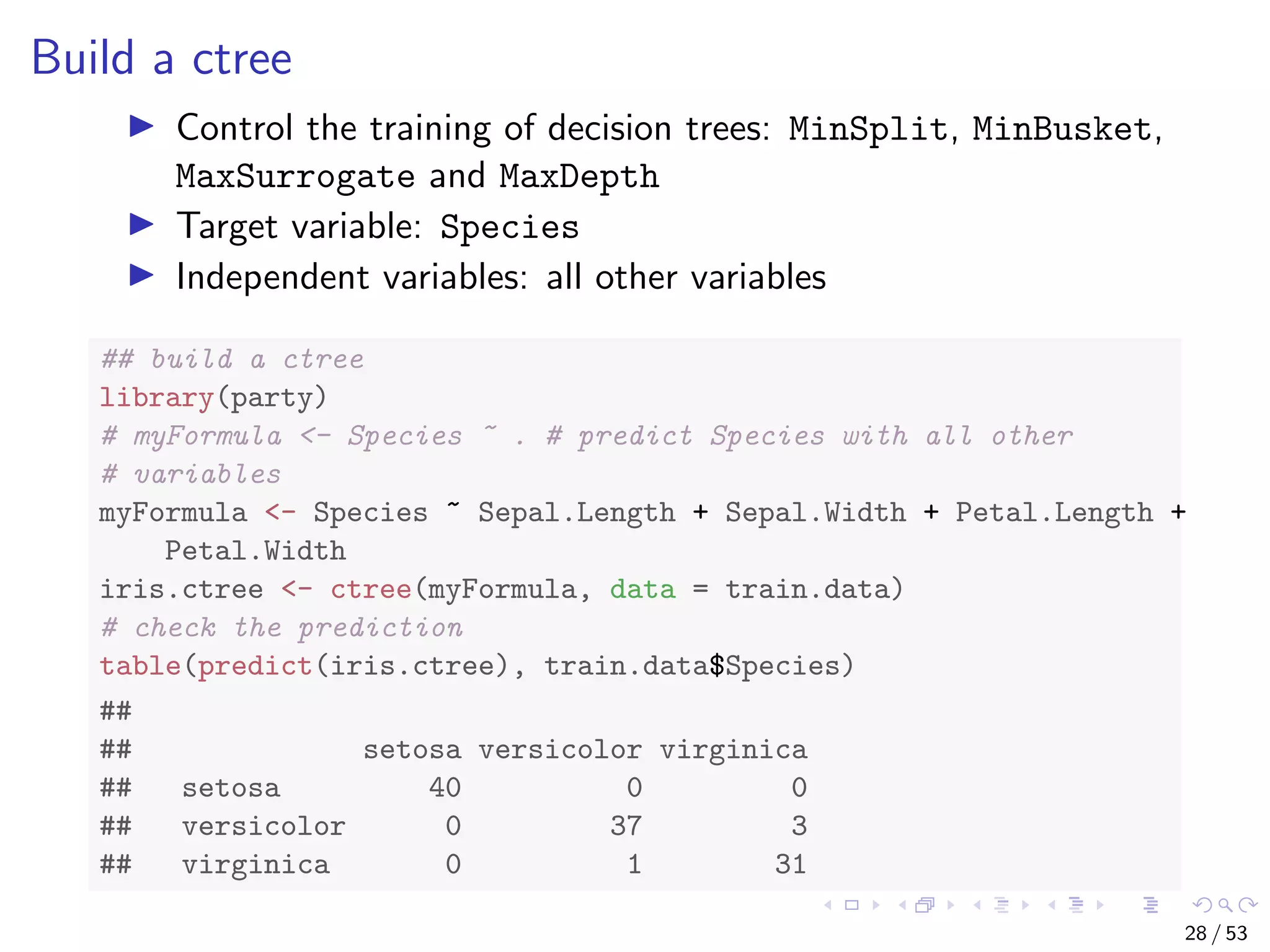
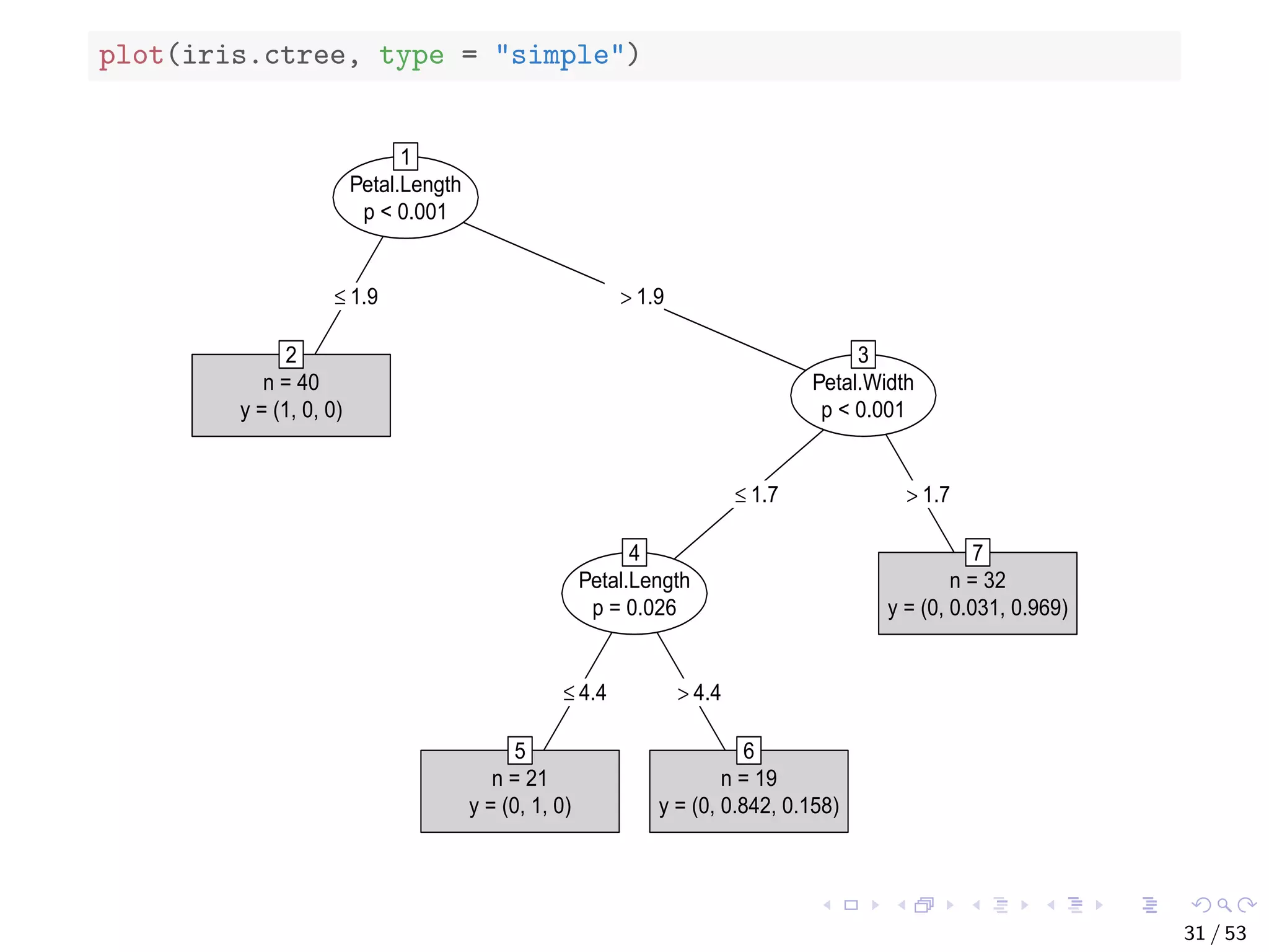
![The iris Data str(iris) ## 'data.frame': 150 obs. of 5 variables: ## $ Sepal.Length: num 5.1 4.9 4.7 4.6 5 5.4 4.6 5 4.4 4.9 ... ## $ Sepal.Width : num 3.5 3 3.2 3.1 3.6 3.9 3.4 3.4 2.9 3.1... ## $ Petal.Length: num 1.4 1.4 1.3 1.5 1.4 1.7 1.4 1.5 1.4 1... ## $ Petal.Width : num 0.2 0.2 0.2 0.2 0.2 0.4 0.3 0.2 0.2 0... ## $ Species : Factor w/ 3 levels "setosa","versicolor",.... # split data into two subsets: training (70%) and test (30%); set # a fixed random seed to make results reproducible set.seed(1234) ind <- sample(2, nrow(iris), replace = TRUE, prob = c(0.7, 0.3)) train.data <- iris[ind == 1, ] test.data <- iris[ind == 2, ] 27 / 53](https://image.slidesharecdn.com/rdm-slides-regression-classification-190703041150/75/RDataMining-slides-regression-classification-28-2048.jpg)
![The bodyfat Dataset ## build a decision tree with rpart data("bodyfat", package = "TH.data") dim(bodyfat) ## [1] 71 10 # str(bodyfat) head(bodyfat, 5) ## age DEXfat waistcirc hipcirc elbowbreadth kneebreadth ## 47 57 41.68 100.0 112.0 7.1 9.4 ## 48 65 43.29 99.5 116.5 6.5 8.9 ## 49 59 35.41 96.0 108.5 6.2 8.9 ## 50 58 22.79 72.0 96.5 6.1 9.2 ## 51 60 36.42 89.5 100.5 7.1 10.0 ## anthro3a anthro3b anthro3c anthro4 ## 47 4.42 4.95 4.50 6.13 ## 48 4.63 5.01 4.48 6.37 ## 49 4.12 4.74 4.60 5.82 ## 50 4.03 4.48 3.91 5.66 ## 51 4.24 4.68 4.15 5.91 34 / 53](https://image.slidesharecdn.com/rdm-slides-regression-classification-190703041150/75/RDataMining-slides-regression-classification-35-2048.jpg)
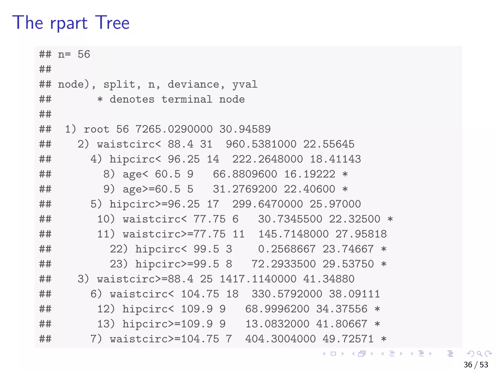
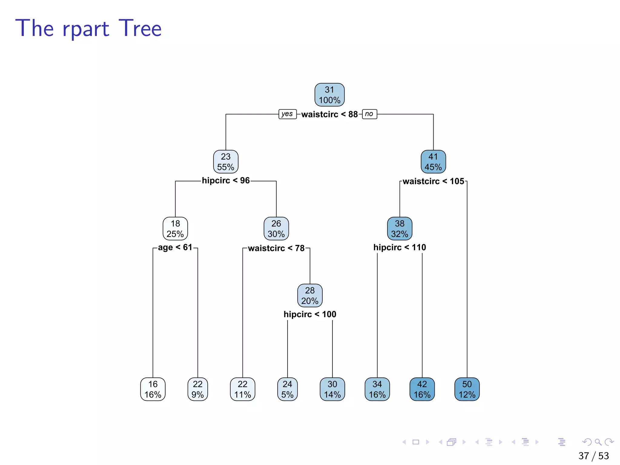
![Train a Decision Tree with Package rpart # split into training and test subsets set.seed(1234) ind <- sample(2, nrow(bodyfat), replace=TRUE, prob=c(0.7, 0.3)) bodyfat.train <- bodyfat[ind==1,] bodyfat.test <- bodyfat[ind==2,] # train a decision tree library(rpart) myFormula <- DEXfat ~ age + waistcirc + hipcirc + elbowbreadth + kneebreadth bodyfat.rpart <- rpart(myFormula, data = bodyfat.train, control = rpart.control(minsplit = 10)) # print(bodyfat.rpart£cptable) library(rpart.plot) rpart.plot(bodyfat.rpart) 35 / 53](https://image.slidesharecdn.com/rdm-slides-regression-classification-190703041150/75/RDataMining-slides-regression-classification-36-2048.jpg)
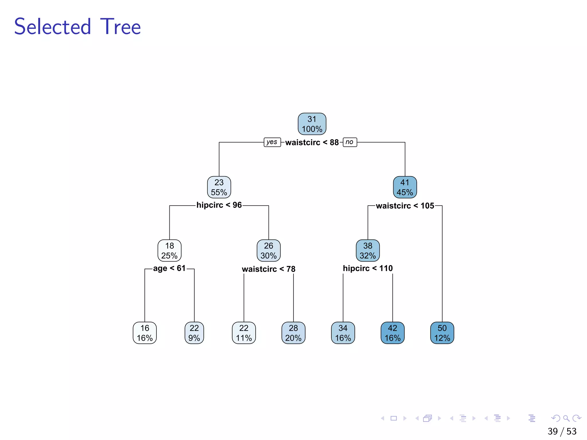
![Select the Best Tree # select the tree with the minimum prediction error opt <- which.min(bodyfat.rpart$cptable[, "xerror"]) cp <- bodyfat.rpart$cptable[opt, "CP"] # prune tree bodyfat.prune <- prune(bodyfat.rpart, cp = cp) # plot tree rpart.plot(bodyfat.prune) 38 / 53](https://image.slidesharecdn.com/rdm-slides-regression-classification-190703041150/75/RDataMining-slides-regression-classification-39-2048.jpg)
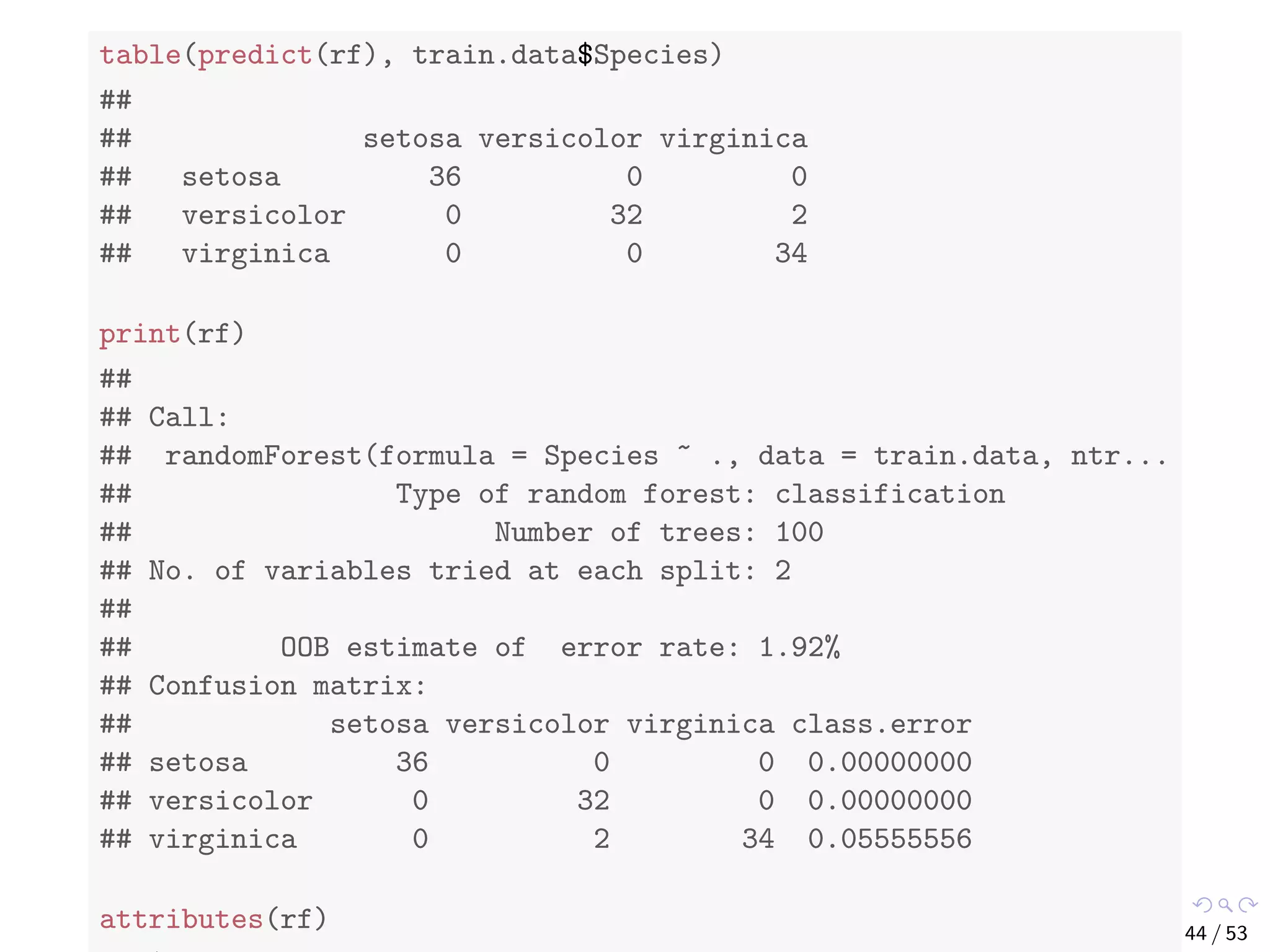
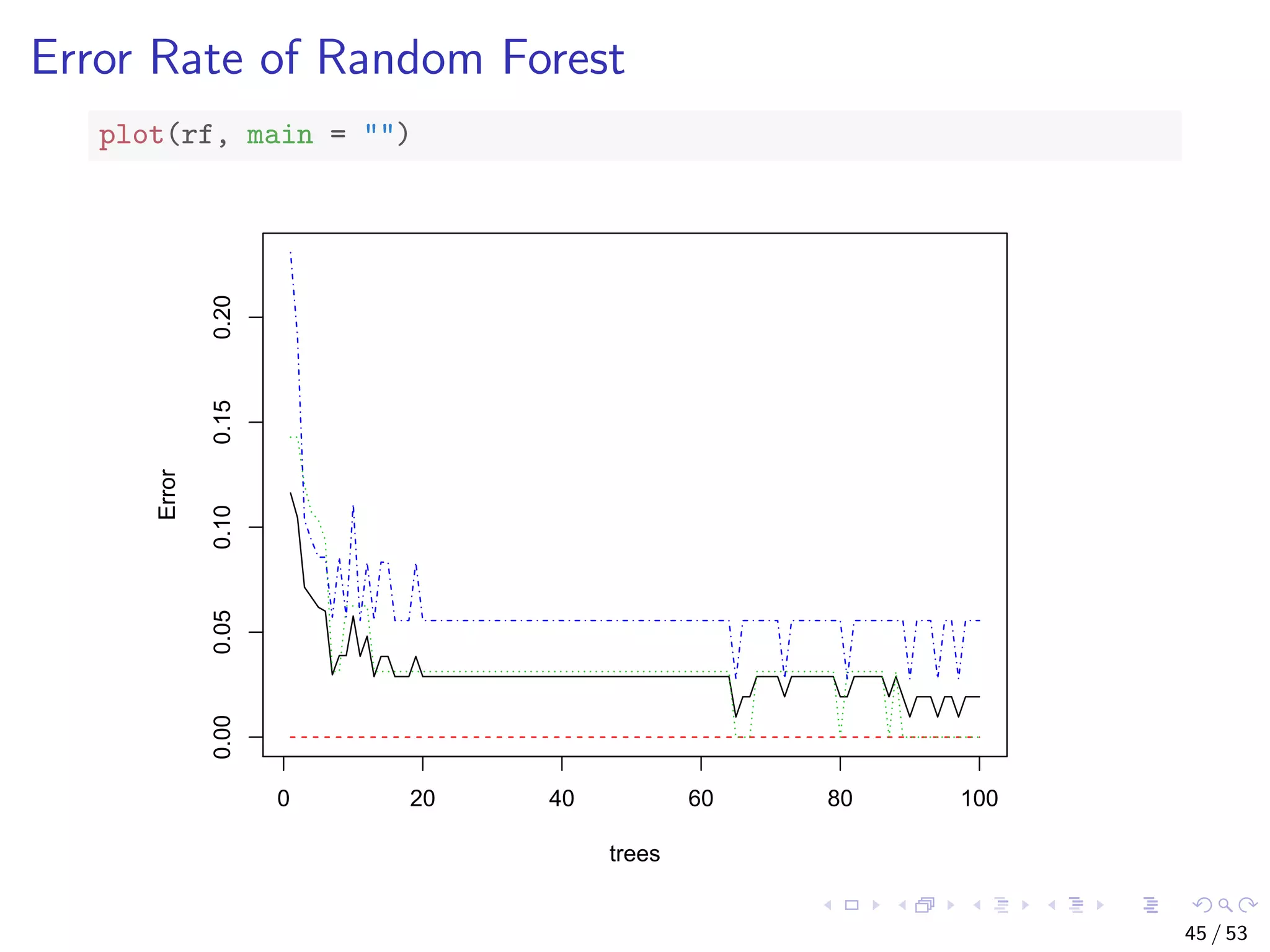
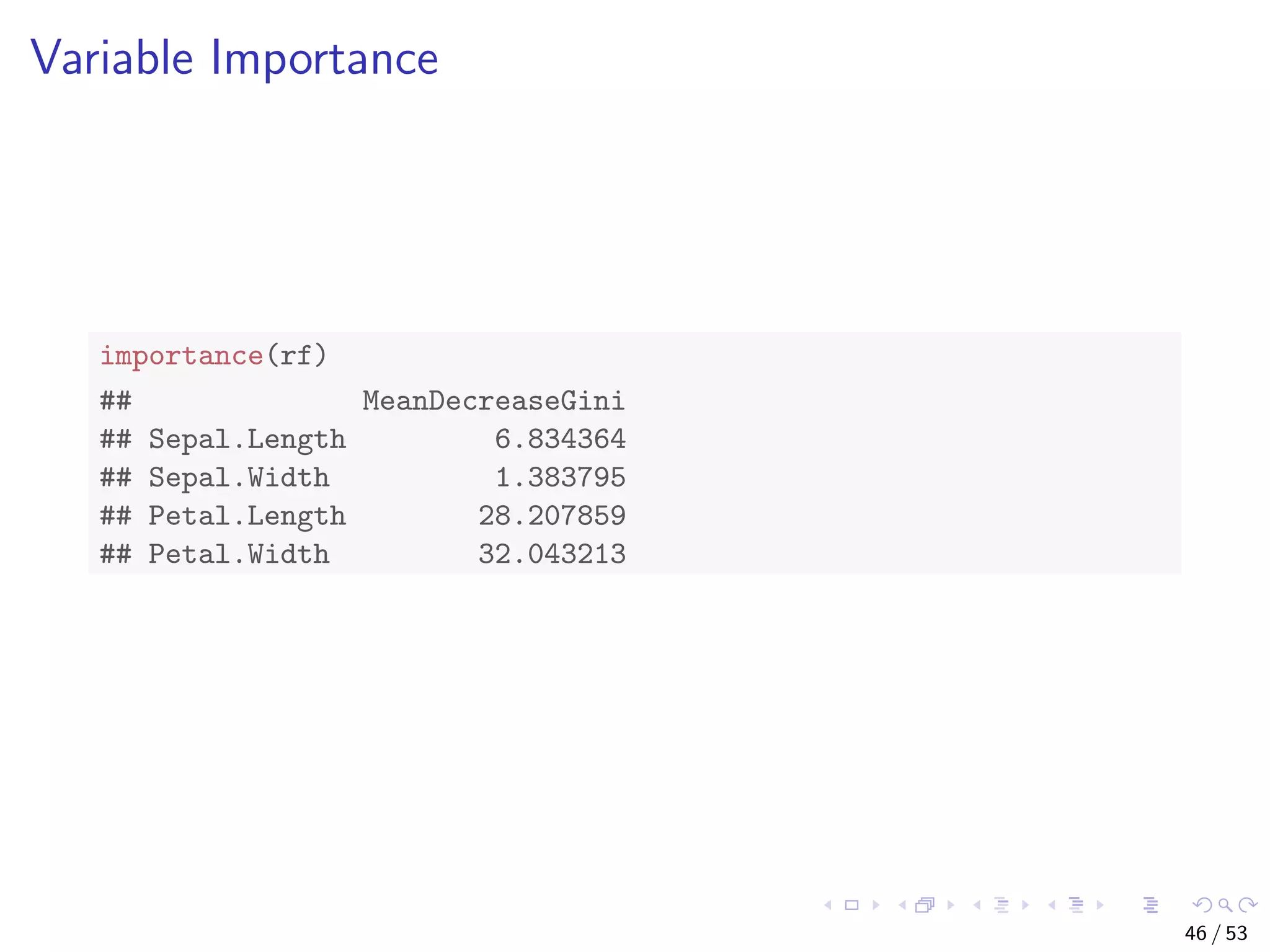
![Train a Random Forest # split into two subsets: training (70%) and test (30%) ind <- sample(2, nrow(iris), replace=TRUE, prob=c(0.7, 0.3)) train.data <- iris[ind==1,] test.data <- iris[ind==2,] # use all other variables to predict Species library(randomForest) rf <- randomForest(Species ~ ., data=train.data, ntree=100, proximity=T) 43 / 53](https://image.slidesharecdn.com/rdm-slides-regression-classification-190703041150/75/RDataMining-slides-regression-classification-44-2048.jpg)

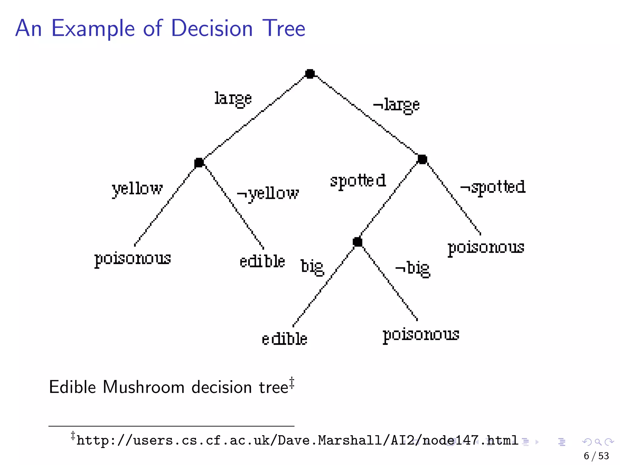
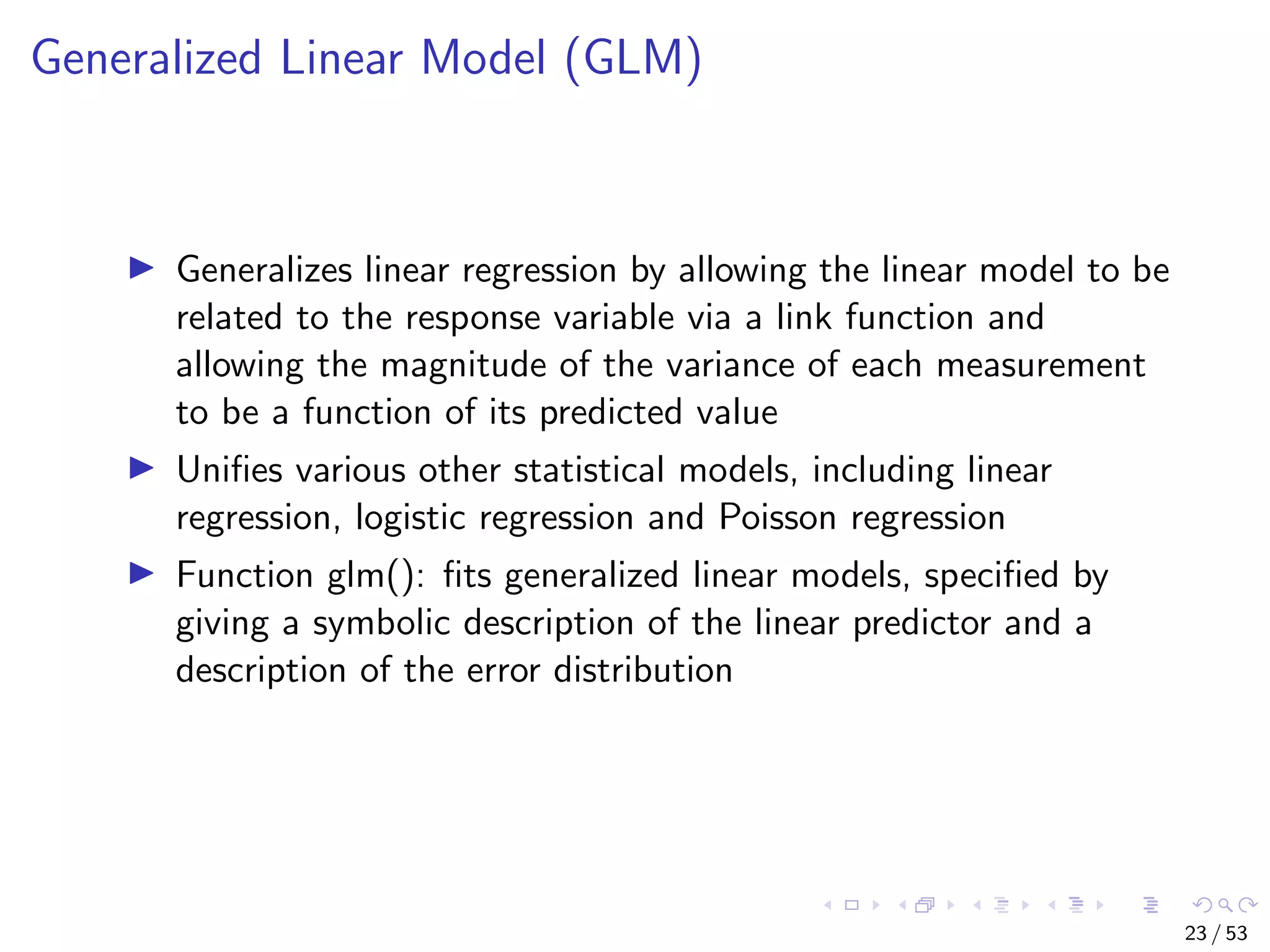
The document describes building regression and classification models in R, including linear regression, generalized linear models, decision trees, and random forests. It uses examples of CPI data to demonstrate linear regression and predicts CPI values in 2011. For classification, it builds a decision tree model on the iris dataset using the party package and visualizes the tree. The document provides information on evaluating and comparing different models.