Download as PDF, PPTX
![R Language I drops whitespace, semi-colons optional but are needed for multiple commands in the same line I comments: # I case sensitive I functional and object oriented programming (a=b rephrased as ’=’(a,b)) I interpreted but with lazy evaluation I not strongly typed I help() displays help on a function, dataset, etc. a = 3.2 a = "a string"; b = 2 # no strong typing print(a) ## [1] "a string"](https://image.slidesharecdn.com/rminicoursecombined-150930180229-lva1-app6891/75/Data-Analysis-with-R-combined-slides-8-2048.jpg)
![q = rep(3.2, times = 10) # repeat value multiple times w = seq(0, 1, by = 0.1) # values in [0,1] in 0.1 increments w = seq(0, 1, length.out = 11) # equally spaced values w <= 0.5 # boolean vector any(w <= 0.5) # is it true for some elements? all(w <= 0.5) # is it true for all elements? which(w <= 0.5) # for which elements is it true? w[w <= 0.5] # extracting from w entries for which w<=0.5 subset(w, w <= 0.5) # an alternative with the subset function w[w <= 0.5] = 0 # zero out all components <= 0.5](https://image.slidesharecdn.com/rminicoursecombined-150930180229-lva1-app6891/75/Data-Analysis-with-R-combined-slides-13-2048.jpg)
![Arrays are multidimensional generalization of vectors. z = seq(1, 20,length.out = 20) # create a vector 1,2,..,20 x = array(data = z, dim = c(4, 5)) # create a 2-d array x[2,3] # refer to the second row and third column x[2,] # refer to the entire second row x[-1,] # all but the first row - same as x[c(2,3,4),] y = x[c(1,2),c(1,2)] # 2x2 top left sub-matrix 2 * y + 1 # element-wise operation y %*% y # matrix product (both arguments are matrices) x[1,] %*% x[1,] # inner product t(x) # matrix transpose outer(x[,1], x[,1]) # outer product rbind(x[1,], x[1,]) # vertical concatenation cbind(x[1,], x[1,]) # horizontal concatenation](https://image.slidesharecdn.com/rminicoursecombined-150930180229-lva1-app6891/75/Data-Analysis-with-R-combined-slides-14-2048.jpg)
![Lists Lists are ordered collections of possibly di↵erent types. Named positions allow creating self-describing data. L=list(name = 'John', age = 55, no.children = 2, children.ages = c(15, 18)) names(L) # displays all position names L[[2]] # second element L[2] # list containing second element L$name # value in list corresponding to name L['name'] # same thing L$children.ages[2] # same as L[[4]][2]](https://image.slidesharecdn.com/rminicoursecombined-150930180229-lva1-app6891/75/Data-Analysis-with-R-combined-slides-15-2048.jpg)
![Datasets Example: Iris dataset (in datasets package) names(iris) # lists the dimension (column) names head(iris, 4) # show first four rows iris[1,] # first row iris$Sepal.Length[1:10] # sepal length of first ten samples # allow replacing iris£Sepal.Length with shorter Sepal.Length attach(iris, warn.conflicts = FALSE) mean(Sepal.Length) # average of Sepal.Length across all rows colMeans(iris[,1:4]) # means of all four numeric columns subset(iris, Sepal.Length < 5 & Species != "setosa") # count number of rows corresponding to setosa species dim(subset(iris, Species == "setosa"))[1] summary(iris)](https://image.slidesharecdn.com/rminicoursecombined-150930180229-lva1-app6891/75/Data-Analysis-with-R-combined-slides-17-2048.jpg)
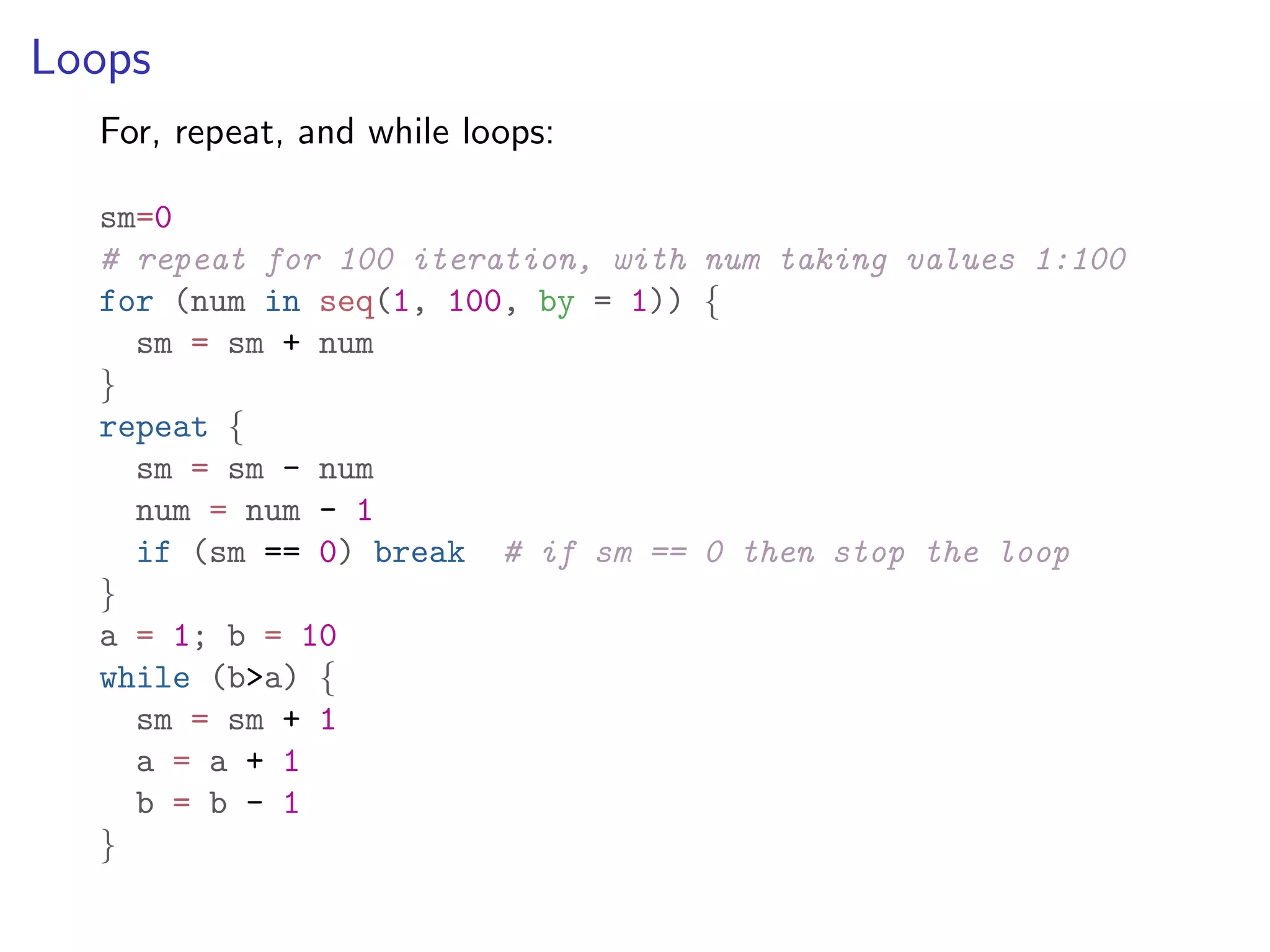
![If-Else a = 10; b = 5; c = 1 if (a < b) { d = 1 } else if (a == b) { d = 2 } else { d = 3 } print(d) ## [1] 3 AND: &&, OR: ||, equality: ==, inequality: !=](https://image.slidesharecdn.com/rminicoursecombined-150930180229-lva1-app6891/75/Data-Analysis-with-R-combined-slides-18-2048.jpg)
![## [1] 13.34 17.48 21.21 24.71 28.03 31.24 34.34 37.37 40.33 43 ## [1] 13.34 17.48 21.21 24.71 28.03 31.24 34.34 37.37 40.33 43 0.0 0.5 1.0 1.5 0 250 500 750 1000 array size computationtime(sec) language C R](https://image.slidesharecdn.com/rminicoursecombined-150930180229-lva1-app6891/75/Data-Analysis-with-R-combined-slides-24-2048.jpg)
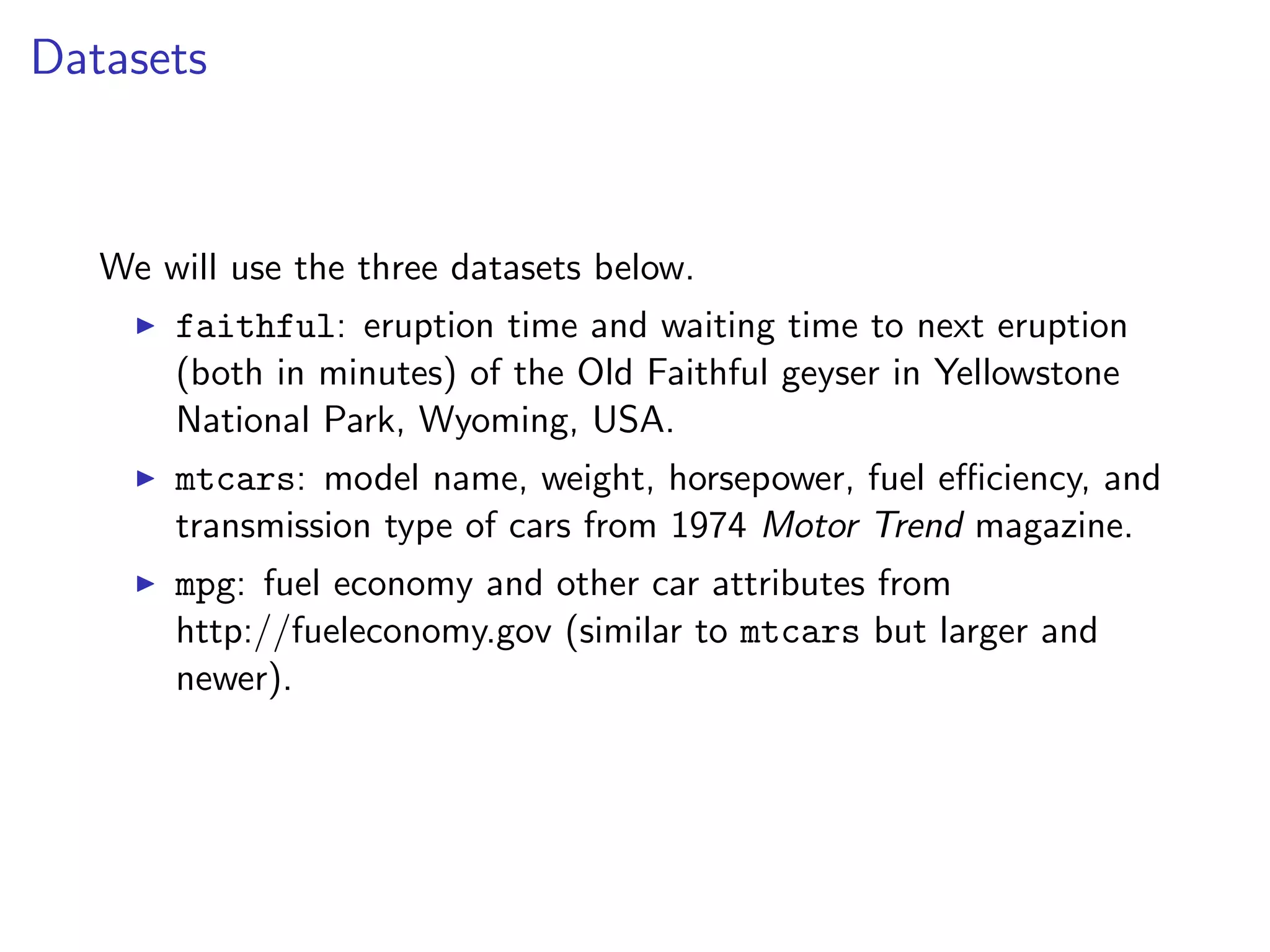
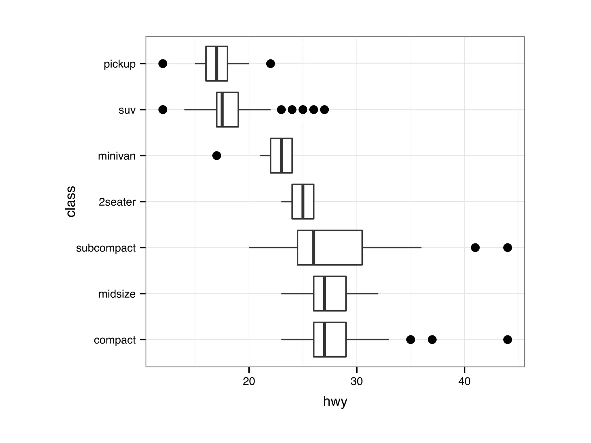
![names(faithful) ## [1] "eruptions" "waiting" names(mtcars) ## [1] "mpg" "cyl" "disp" "hp" "drat" "wt" "qsec" "vs" ## [11] "carb" names(mpg) ## [1] "manufacturer" "model" "displ" "year" ## [5] "cyl" "trans" "drv" "cty" ## [9] "hwy" "fl" "class"](https://image.slidesharecdn.com/rminicoursecombined-150930180229-lva1-app6891/75/Data-Analysis-with-R-combined-slides-31-2048.jpg)
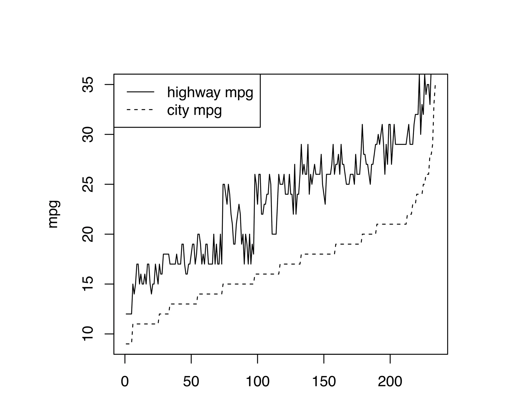
![S = sort.int(mpg$cty, index.return = T) # x: city mpg # ix: indices of sorted values of city mpg plot(S$x, # plot sorted city mpg values with a line plot type = "l", lty = 2, xlab = "sample number (sorted by city mpg)", ylab = "mpg") lines(mpg$hwy[S$ix] ,lty = 1) # add dashed line of hwy mpg legend("topleft", c("highway mpg", "city mpg"), lty = c(1, 2))](https://image.slidesharecdn.com/rminicoursecombined-150930180229-lva1-app6891/75/Data-Analysis-with-R-combined-slides-42-2048.jpg)
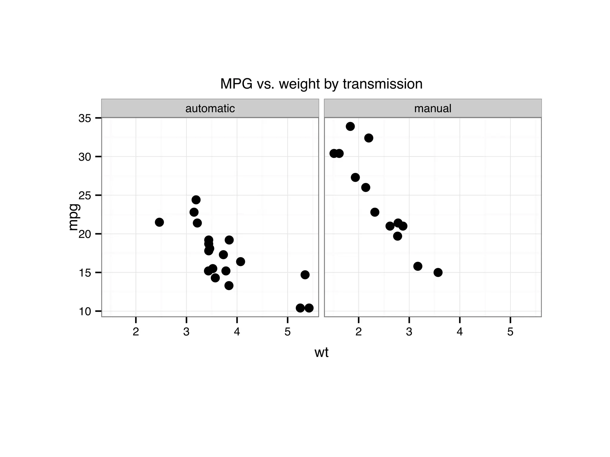
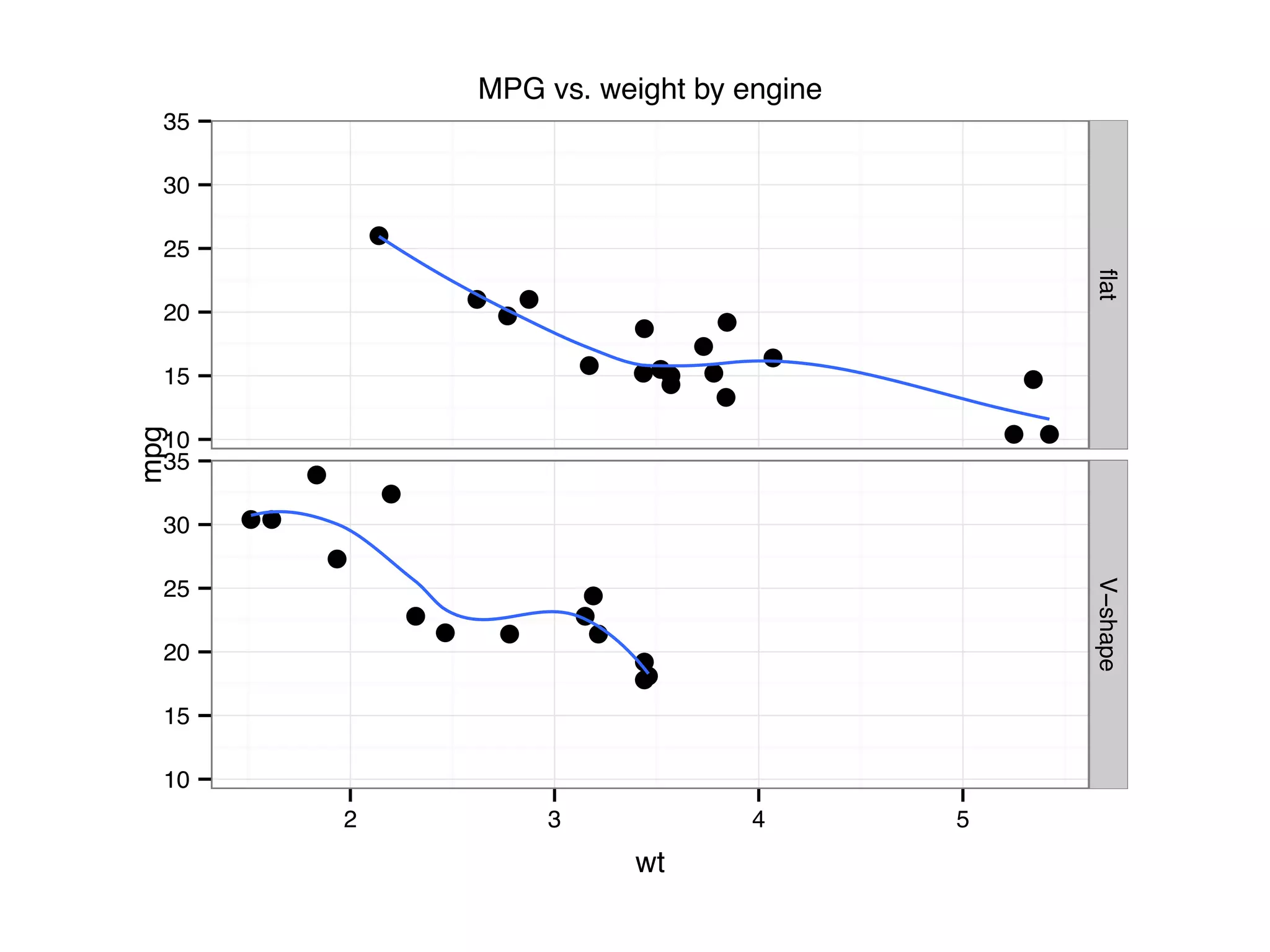
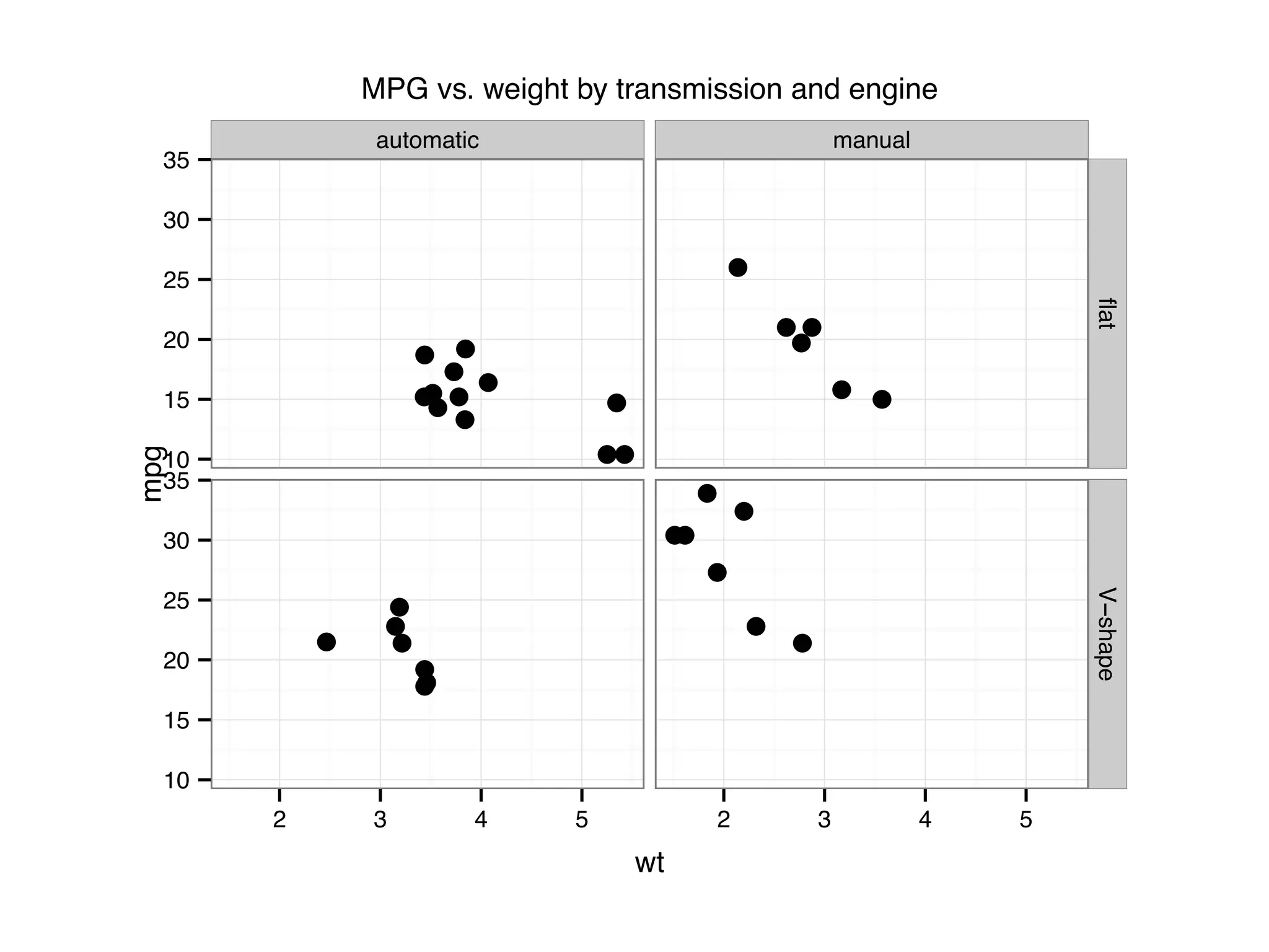
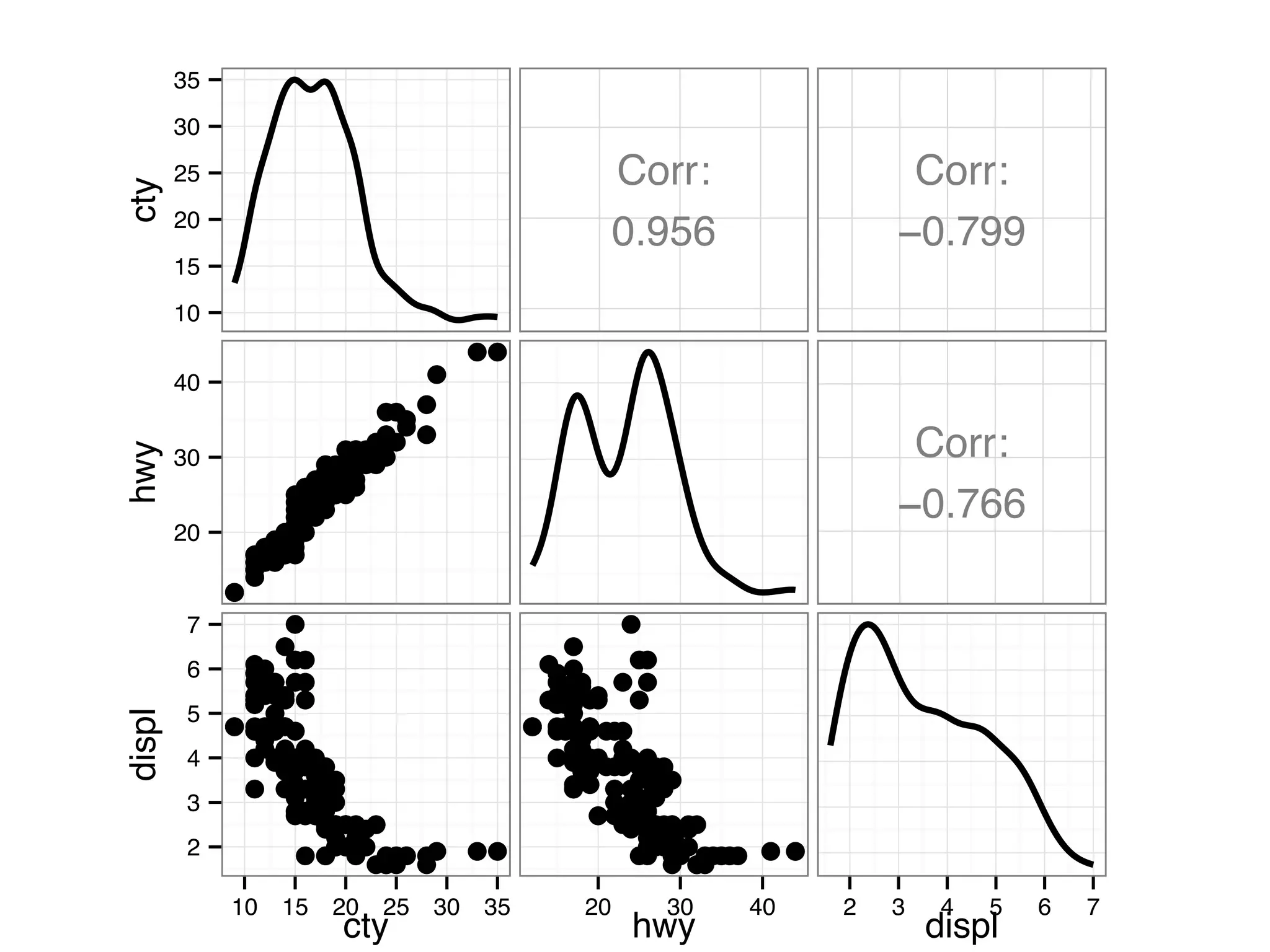
![I Manual transmission cars tend to have lower weights and be more fuel e cient I Cars with V-shape engines tend to weigh less and be more fuel e cient I Manual transmission and V-engine cars tend to be lighter and more fuel e cient. Automatic transmission and non V-engine are heavier and less fuel e cient. “All pairs” plot: DF = mpg[, c("cty", "hwy", "displ")] library(GGally) ggpairs(DF)](https://image.slidesharecdn.com/rminicoursecombined-150930180229-lva1-app6891/75/Data-Analysis-with-R-combined-slides-67-2048.jpg)
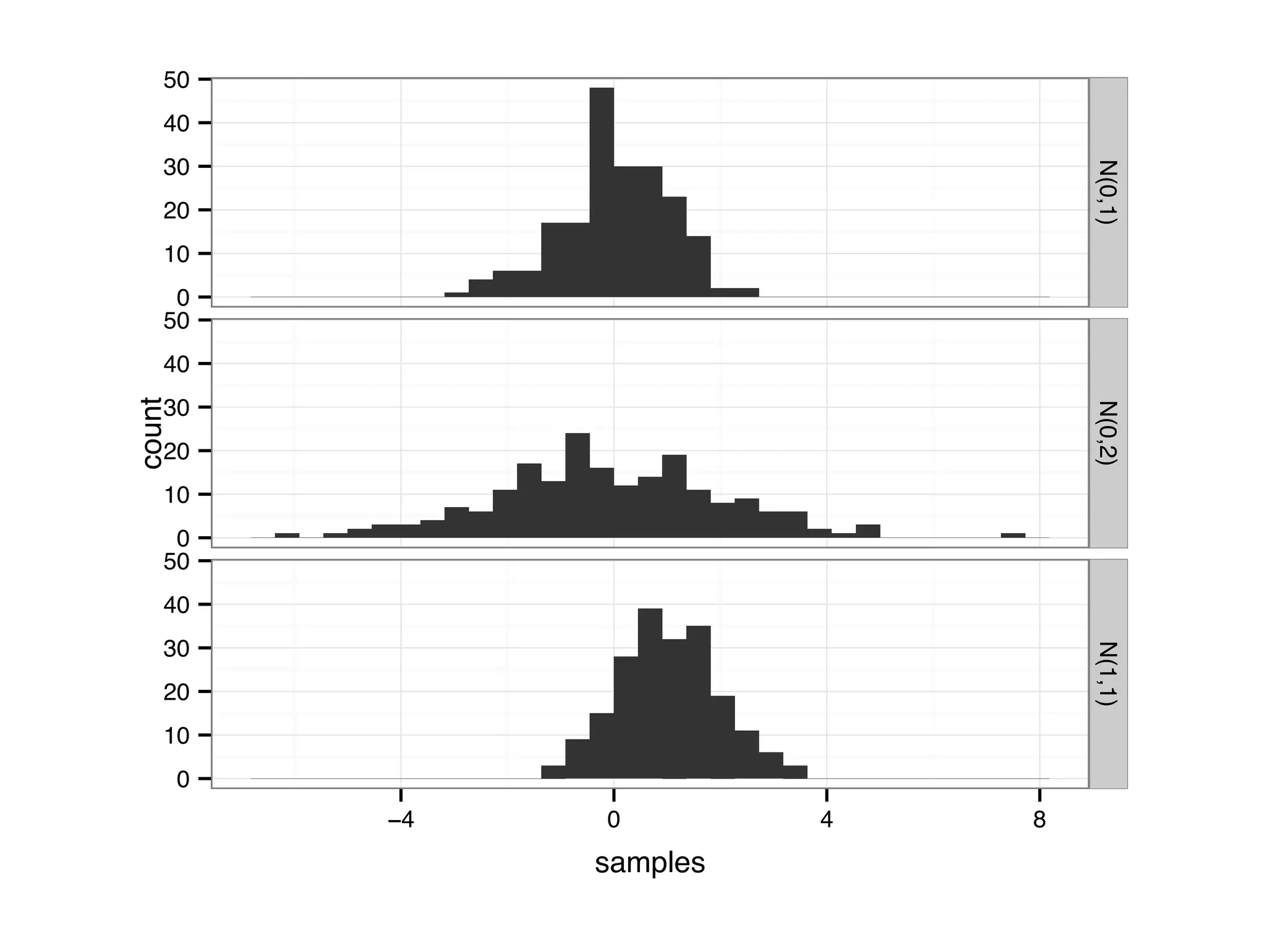
![D = data.frame(samples = c(rnorm(200, 1, 1), rnorm(200, 0, 1), rnorm(200, 0, 2))) D$parameter[1:200] = 'N(1,1)'; D$parameter[201:400] = 'N(0,1)'; D$parameter[401:600] = 'N(0,2)'; qplot(samples, facets = parameter~., geom = 'histogram', data = D)](https://image.slidesharecdn.com/rminicoursecombined-150930180229-lva1-app6891/75/Data-Analysis-with-R-combined-slides-79-2048.jpg)
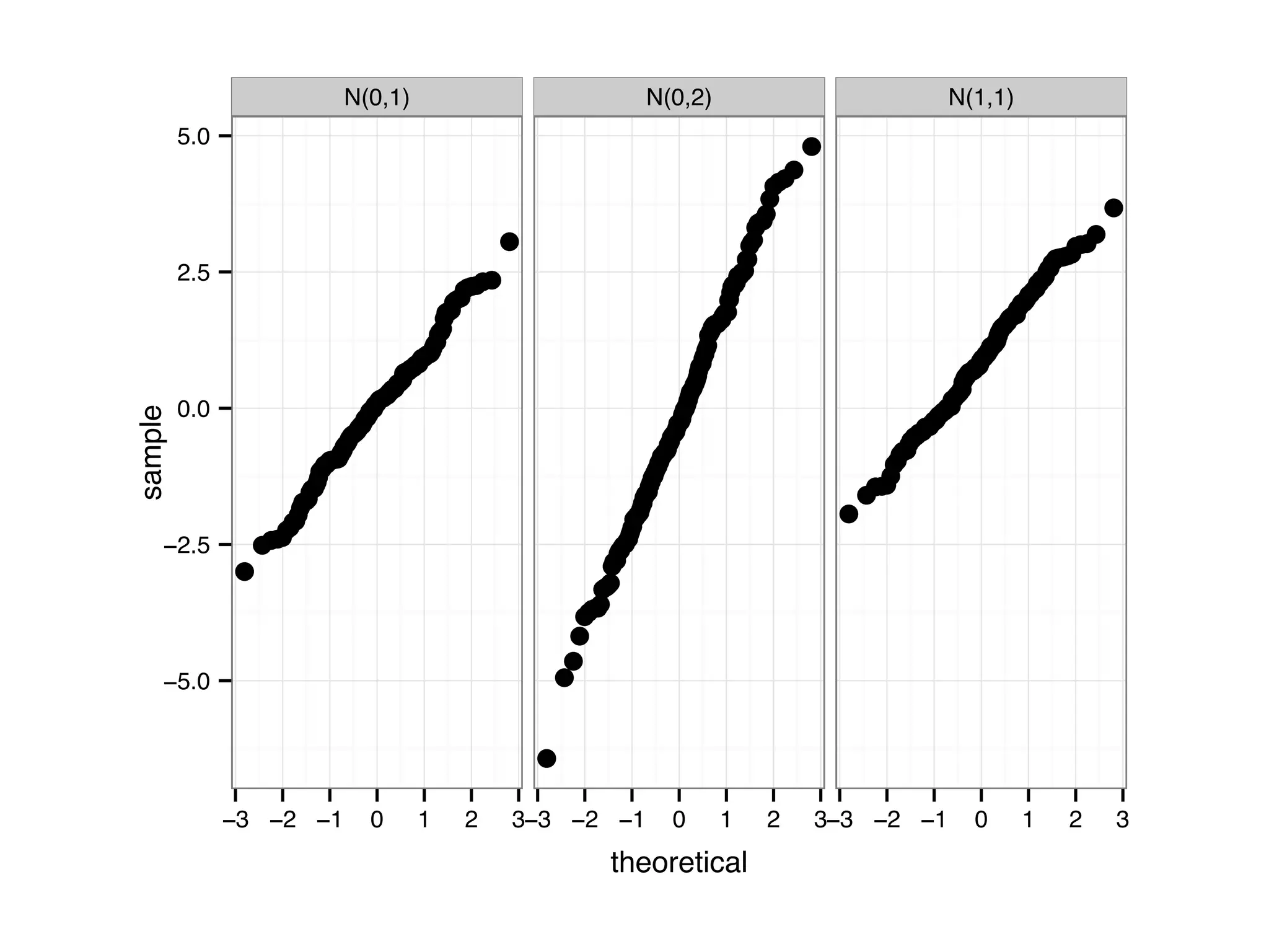
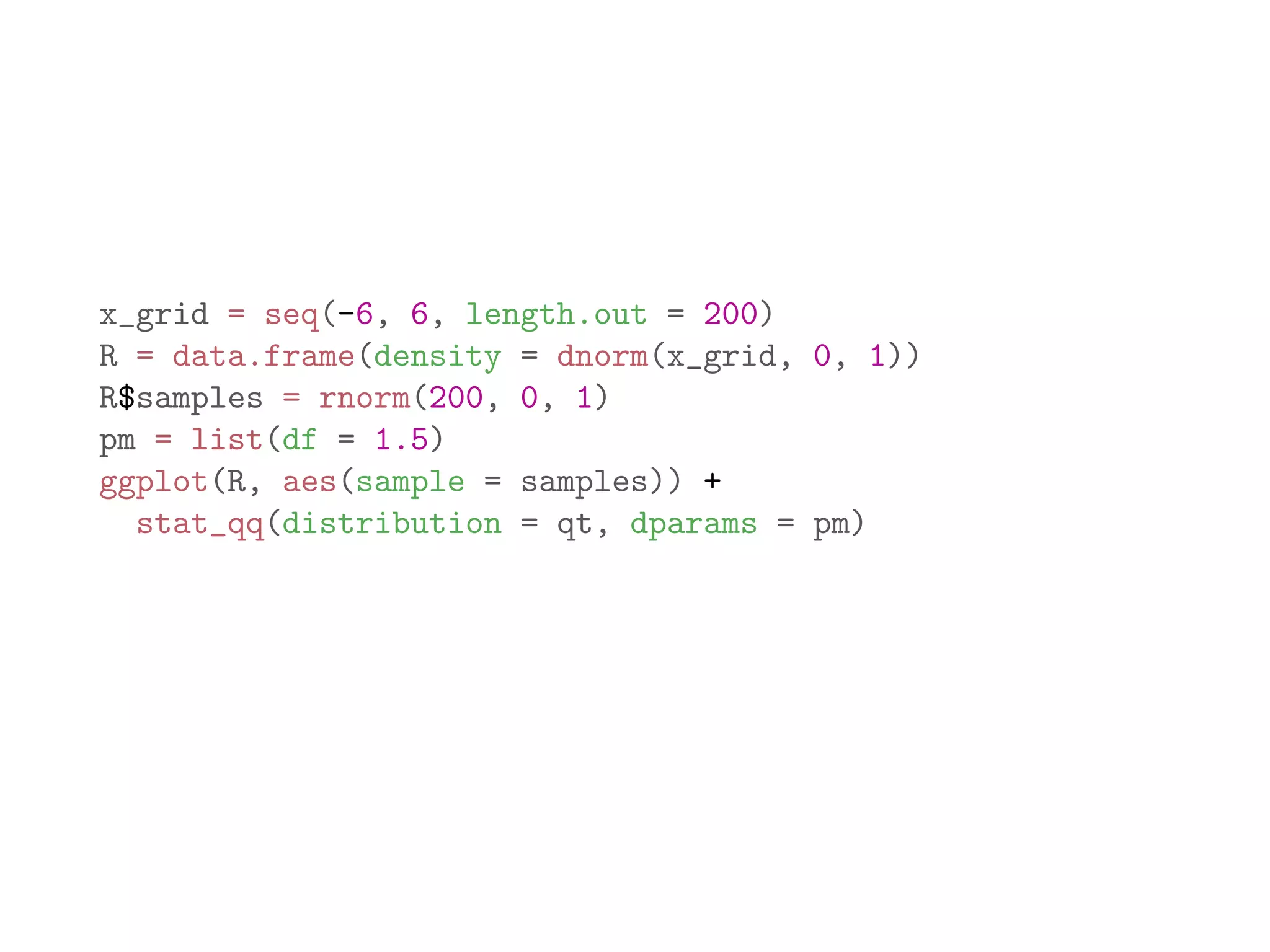
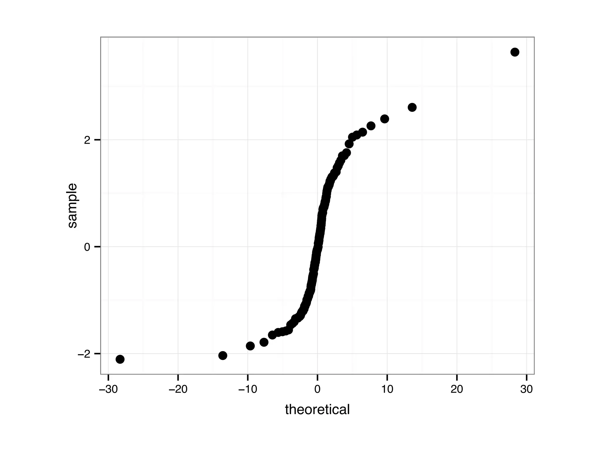
![D = data.frame(samples = c(rnorm(200, 1, 1), rnorm(200, 0, 1), rnorm(200, 0, 2))); D$parameter[1:200] = 'N(1,1)'; D$parameter[201:400] = 'N(0,1)'; D$parameter[401:600] = 'N(0,2)'; ggplot(D, aes(sample = samples)) + stat_qq() + facet_grid(.~parameter)](https://image.slidesharecdn.com/rminicoursecombined-150930180229-lva1-app6891/75/Data-Analysis-with-R-combined-slides-81-2048.jpg)
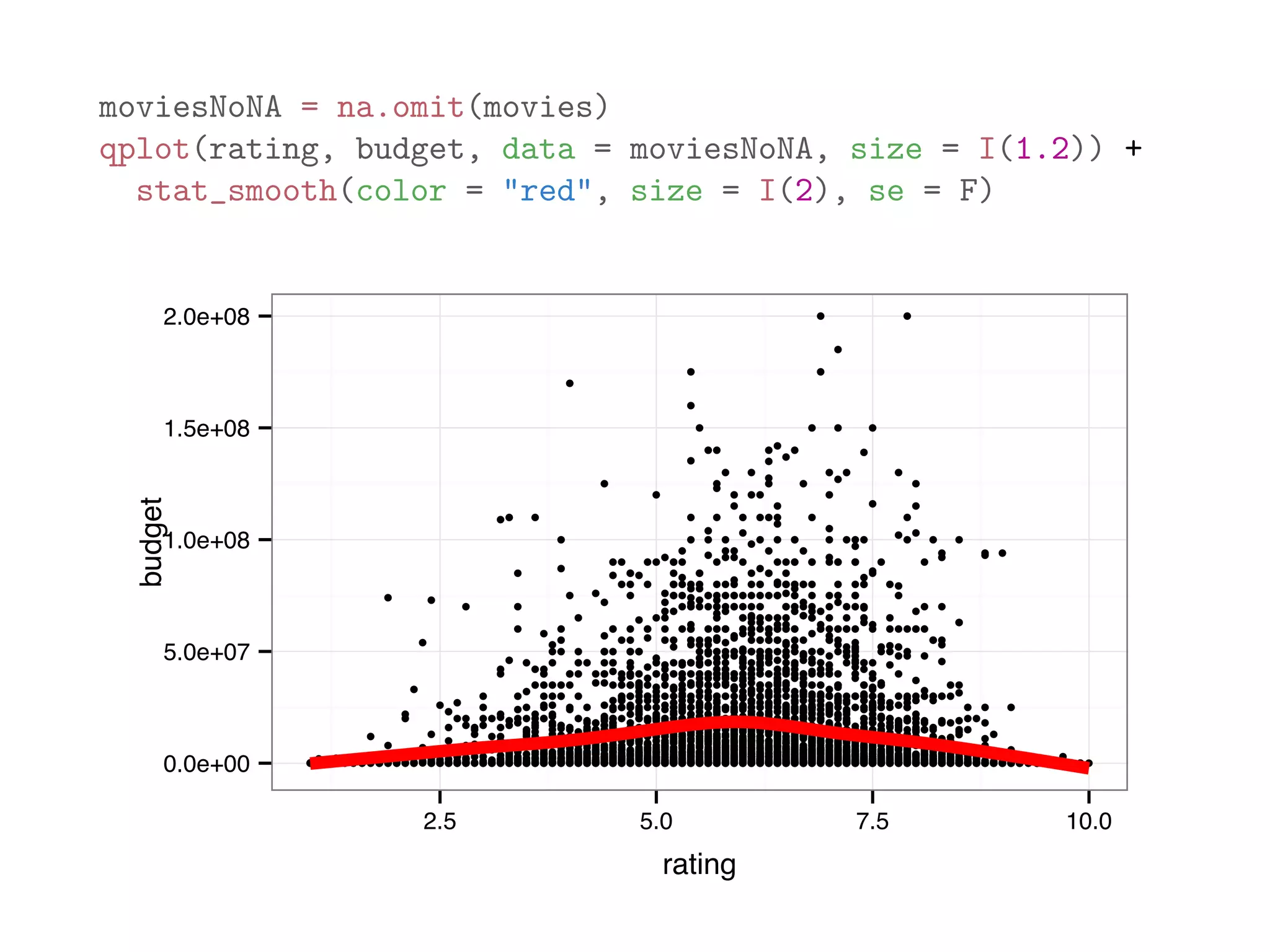
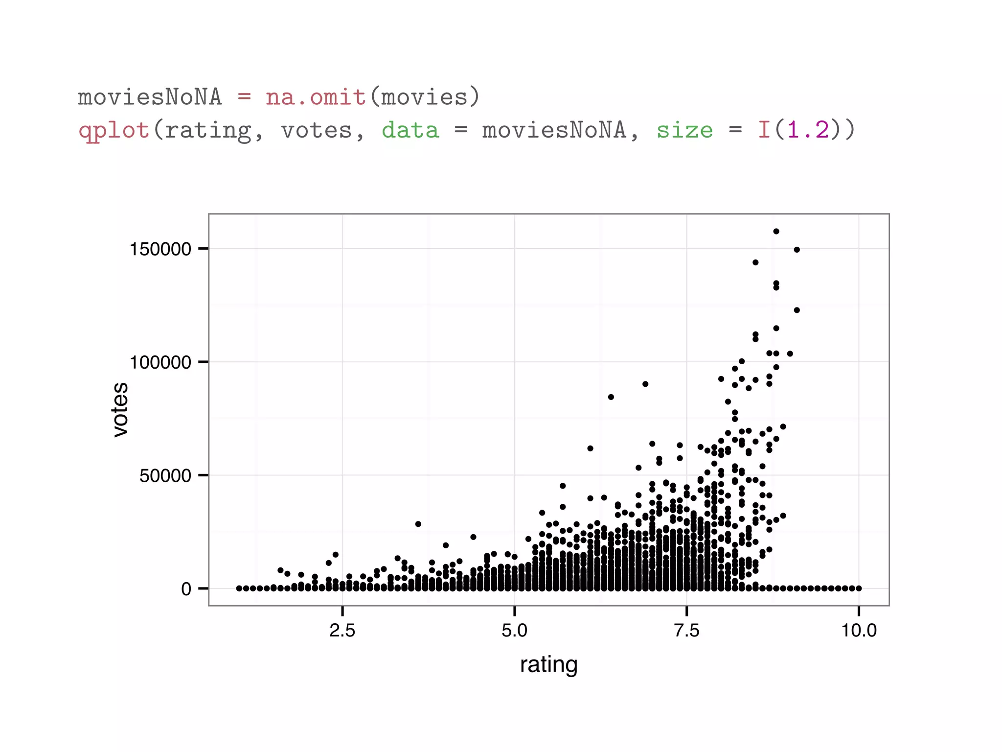
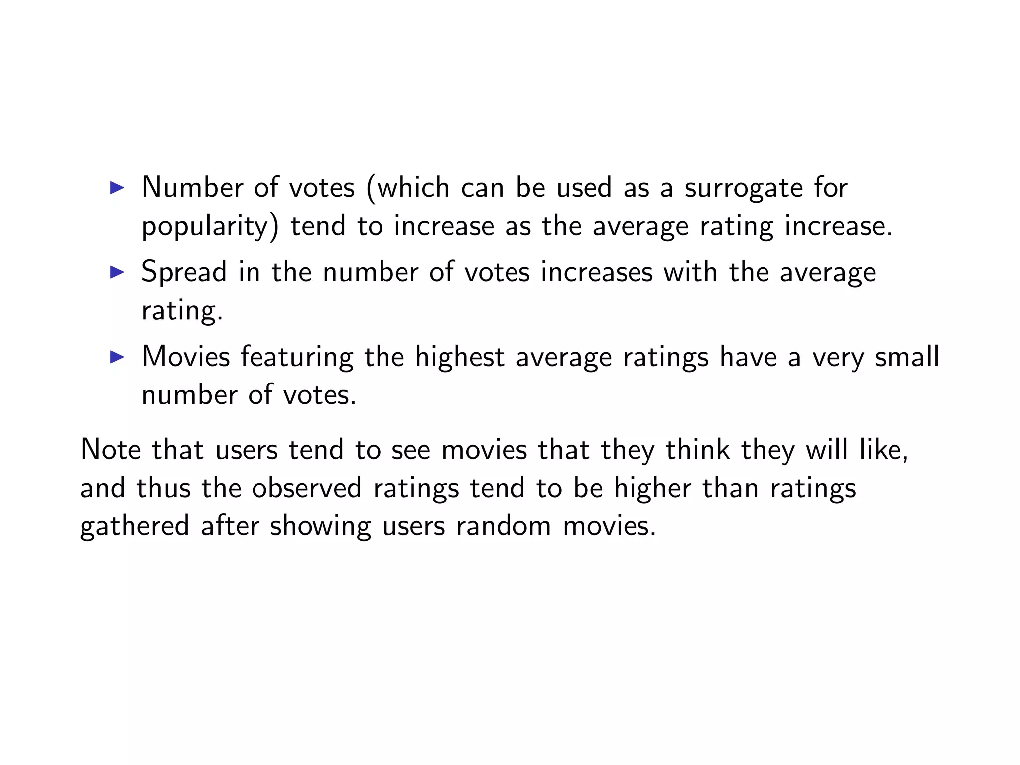
![The code below analyzes the dataframe movies in the ggplot2 package, which contains 24 attributes (genre, year, budget, user ratings, etc.) for 58788 movies obtained from the website http://www.imdb.com with some missing values. mean(movies$length) # average length ## [1] 82.34 mean(movies$budget) # average budget ## [1] NA # average budget (removing missing values) mean(movies$budget, na.rm = TRUE) ## [1] 13412513 mean(is.na(movies$budget)) # frequency of non-missing budget ## [1] 0.9113](https://image.slidesharecdn.com/rminicoursecombined-150930180229-lva1-app6891/75/Data-Analysis-with-R-combined-slides-95-2048.jpg)
![originalData = rnorm(20) originalData[1] = 1000 sortedData = sort(originalData) originalData = originalData[3:18] lowerLimit = mean(sortedData) - 5 * sd(sortedData) upperLimit = mean(sortedData) + 5 * sd(sortedData) noOutlierInd = (lowerLimit < originalData) & (originalData < upperLimit) dataWithoutOutliers = originalData[noOutlierInd]](https://image.slidesharecdn.com/rminicoursecombined-150930180229-lva1-app6891/75/Data-Analysis-with-R-combined-slides-105-2048.jpg)
![library(robustHD) originalData = c(1000, rnorm(10)) print(originalData[1:5]) ## [1] 1000.0000 -0.6265 0.1836 -0.8356 1.5953 print(winsorize(originalData[1:5])) ## [1] 3.2060 -0.6265 0.1836 -0.8356 1.5953](https://image.slidesharecdn.com/rminicoursecombined-150930180229-lva1-app6891/75/Data-Analysis-with-R-combined-slides-106-2048.jpg)
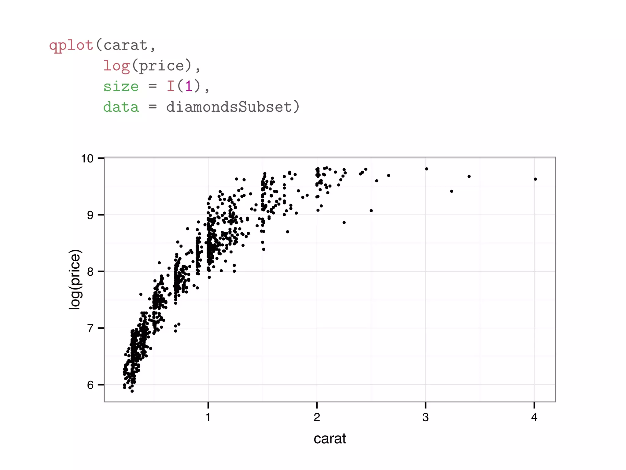
![print(diamonds[1:10,1:8]) ## carat cut color clarity depth table price x ## 1 0.23 Ideal E SI2 61.5 55 326 3.95 ## 2 0.21 Premium E SI1 59.8 61 326 3.89 ## 3 0.23 Good E VS1 56.9 65 327 4.05 ## 4 0.29 Premium I VS2 62.4 58 334 4.20 ## 5 0.31 Good J SI2 63.3 58 335 4.34 ## 6 0.24 Very Good J VVS2 62.8 57 336 3.94 ## 7 0.24 Very Good I VVS1 62.3 57 336 3.95 ## 8 0.26 Very Good H SI1 61.9 55 337 4.07 ## 9 0.22 Fair E VS2 65.1 61 337 3.87 ## 10 0.23 Very Good H VS1 59.4 61 338 4.00](https://image.slidesharecdn.com/rminicoursecombined-150930180229-lva1-app6891/75/Data-Analysis-with-R-combined-slides-109-2048.jpg)
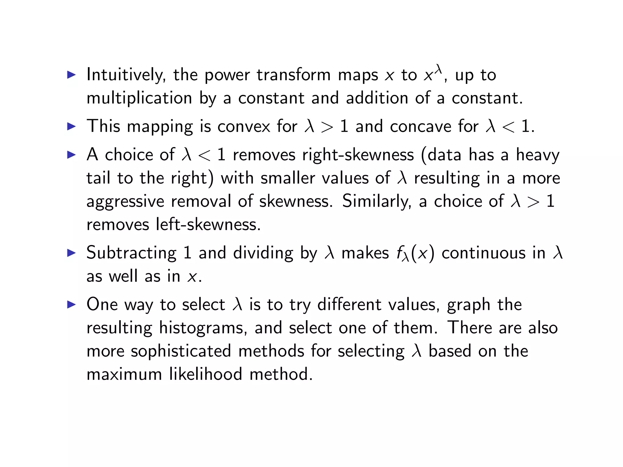
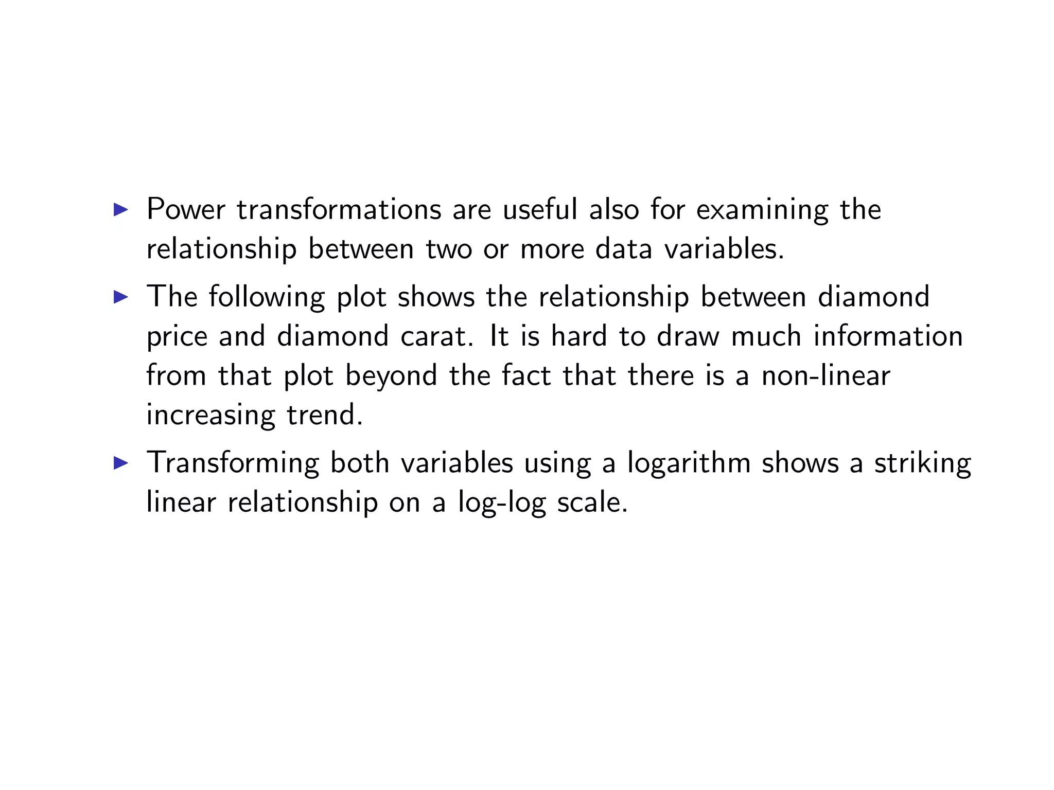
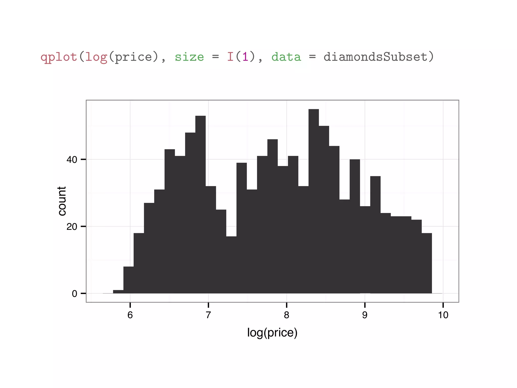
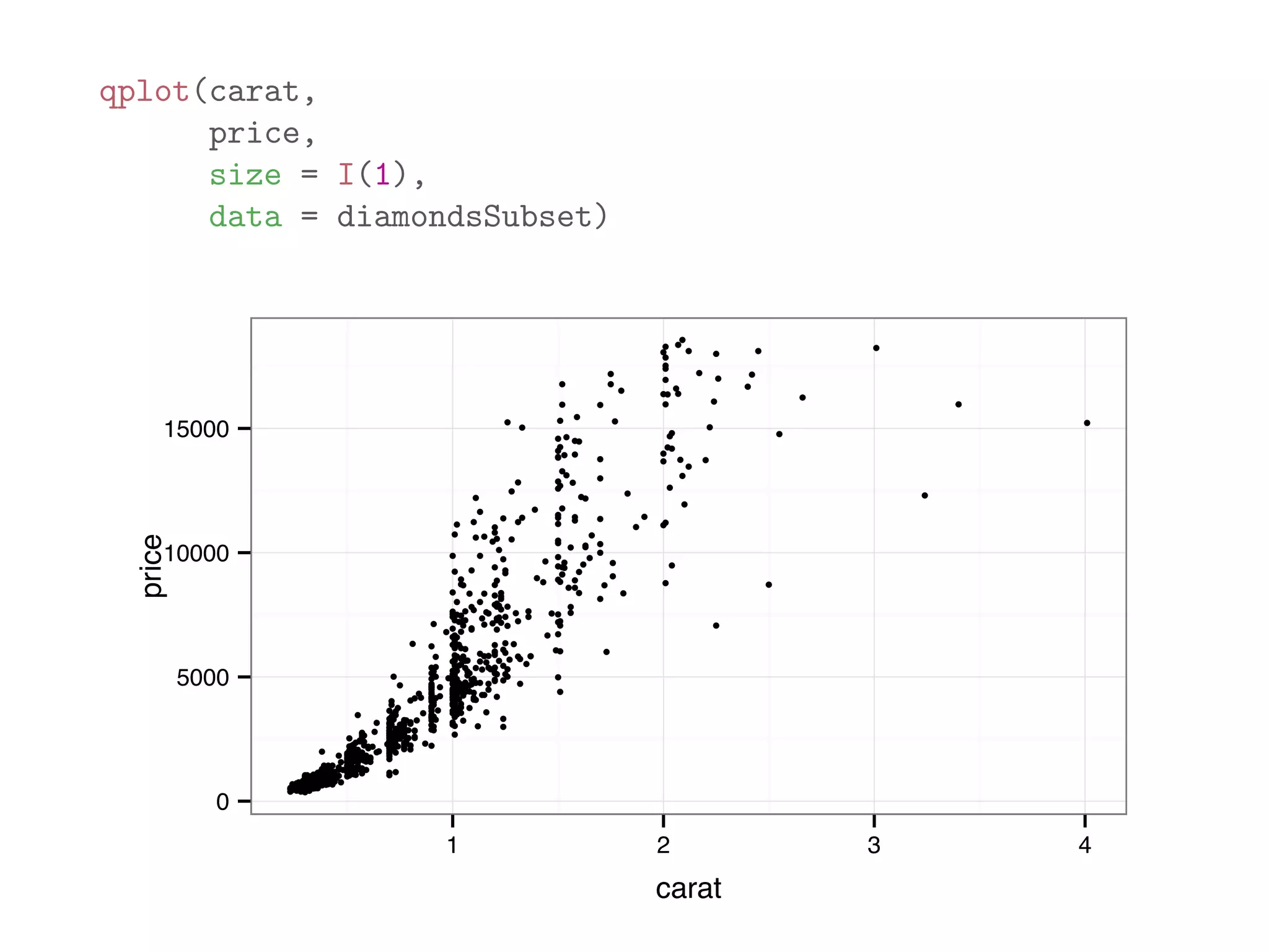
![diamondsSubset = diamonds[sample(dim(diamonds)[1], 1000),] qplot(price, data = diamondsSubset) 0 50 100 150 200 0 5000 10000 15000 20000 price count](https://image.slidesharecdn.com/rminicoursecombined-150930180229-lva1-app6891/75/Data-Analysis-with-R-combined-slides-110-2048.jpg)

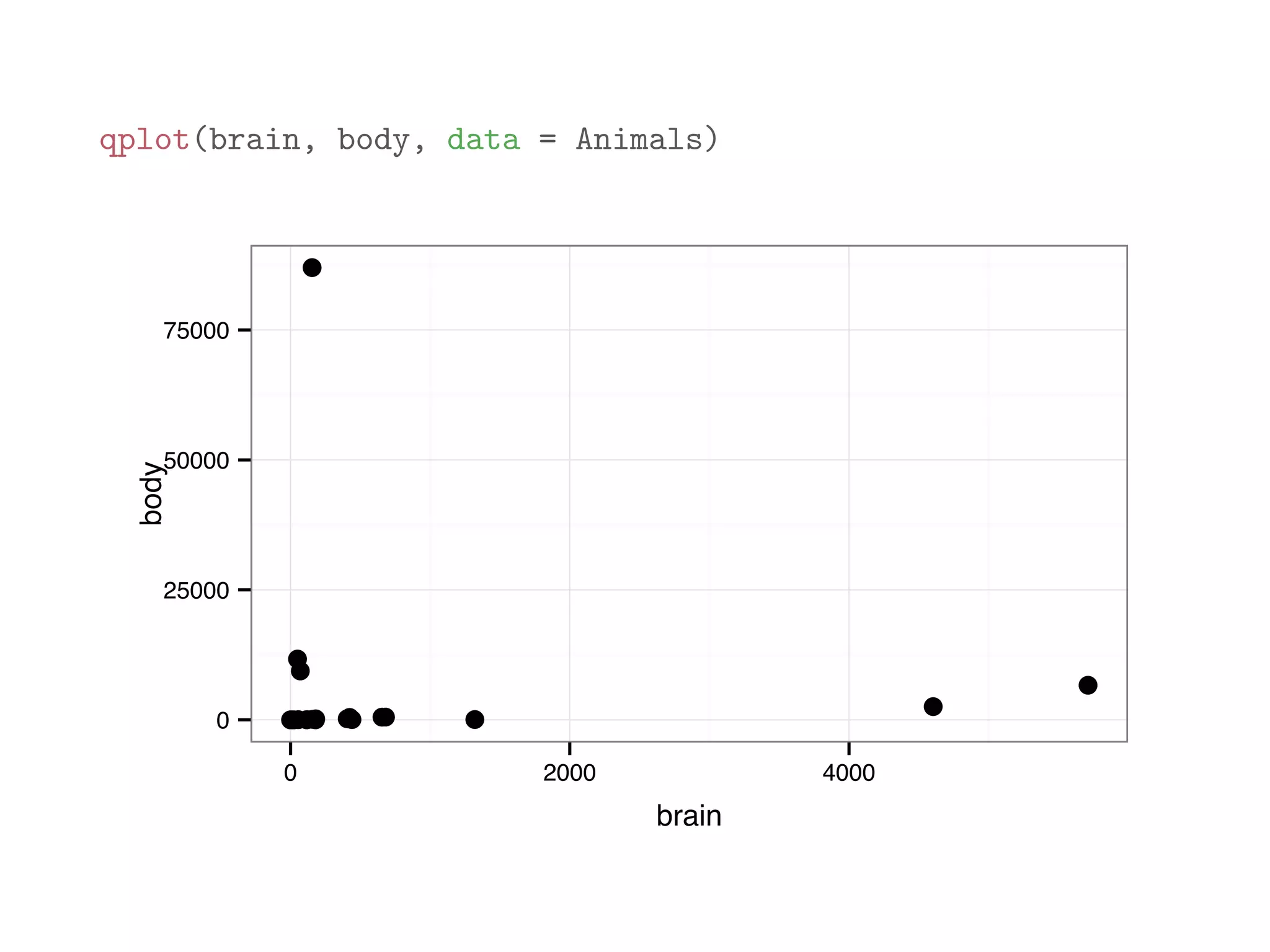
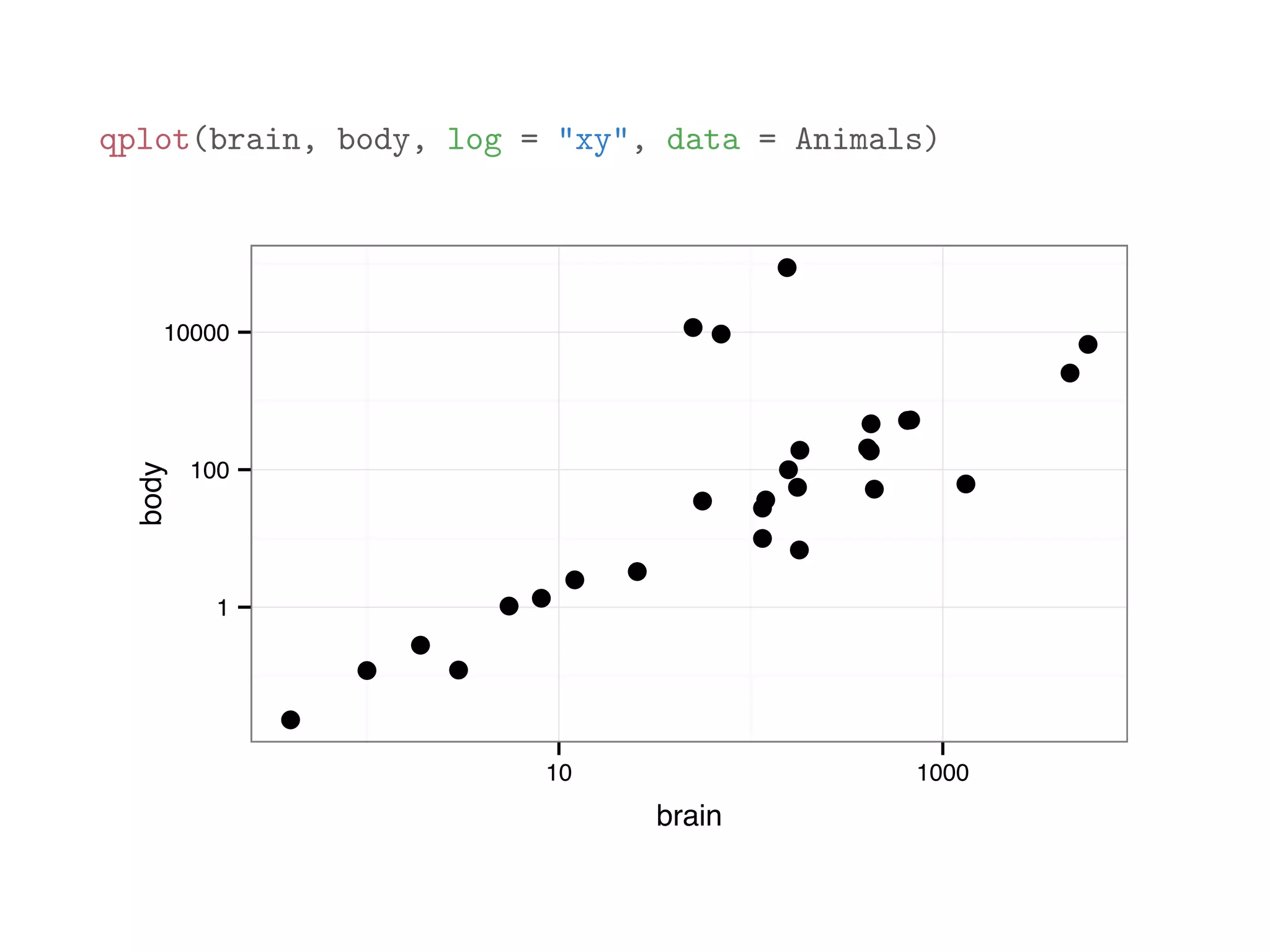
![library(MASS) print(Animals[1:12,]) ## body brain ## Mountain beaver 1.35 8.1 ## Cow 465.00 423.0 ## Grey wolf 36.33 119.5 ## Goat 27.66 115.0 ## Guinea pig 1.04 5.5 ## Dipliodocus 11700.00 50.0 ## Asian elephant 2547.00 4603.0 ## Donkey 187.10 419.0 ## Horse 521.00 655.0 ## Potar monkey 10.00 115.0 ## Cat 3.30 25.6 ## Giraffe 529.00 680.0](https://image.slidesharecdn.com/rminicoursecombined-150930180229-lva1-app6891/75/Data-Analysis-with-R-combined-slides-118-2048.jpg)
![I For example, suppose x represent the tenure of an employee (in years) and ranges from 0 to 50. I A binning process may divide the range [0, 50] into the following ranges (0, 10], (10, 20], . . . , (41, 50] and use corresponding replacement values of 5, 15, . . . , 45 respectively. I The notation (a, b] corresponds to all values larger than a and smaller or equal to b. Discretization in R can be done via the function cut.](https://image.slidesharecdn.com/rminicoursecombined-150930180229-lva1-app6891/75/Data-Analysis-with-R-combined-slides-123-2048.jpg)
![Data Transformations: Indicator Variables I Replace a variable x (numeric, ordinal, or categorical) taking k values with a binary k-dimensional vector v, such that v[i] (or vi in mathematical notation) is one if and only if x takes on the i-value in its range. I Replace variable by vector that is all zeros, except for one component that equals one. I Often, indicator variables are used in conjunction with binning: bin the variable into k bins and then create a k dimensional indicator variable. I High dimensional indicator vectors may be easily handled in computations by taking advantage of its extreme sparsity.](https://image.slidesharecdn.com/rminicoursecombined-150930180229-lva1-app6891/75/Data-Analysis-with-R-combined-slides-124-2048.jpg)
![Data Manipulations: Shu✏ing I A common operation in data analysis is to select a random subset of the rows of a dataframe, with or without replacement. I sample() accepts a vector of values from which to sample (typically a vector of row indices), the number of samples, whether the sampling is done with or without replacement, and the probability of sampling di↵erent values. I sample(k,k) generates a random permutation of order k. I After obtaining the indices that we wish to sample. we form a new array or dataframe containing the sampled rows of the original dataframe. D = array(data = seq(1, 20, length.out = 20), dim = c(4, 5)) D_shuffled = D[sample(4, 4),]](https://image.slidesharecdn.com/rminicoursecombined-150930180229-lva1-app6891/75/Data-Analysis-with-R-combined-slides-126-2048.jpg)
![Data Manipulations: Partitioning I In some cases, we need to partition the dataset’s rows into two or more collection of rows. I Generate a random permutation of k objects (using sample(k,k)), where k is the number of rows in the data, and then divide the permutation vector into two or more parts based on the prescribed sizes, and new dataframes whose rows correspond to the divided permutation vector. D = array(data = seq(1, 20, length.out = 20), dim = c(4, 5)) rand_perm = sample(4,4) first_set_of_indices = rand_perm[1:floor(4*0.75)] second_set_of_indices = rand_perm[(floor(4*0.75)+1):4] D1 = D[first_set_of_indices,] D2 = D[second_set_of_indices,]](https://image.slidesharecdn.com/rminicoursecombined-150930180229-lva1-app6891/75/Data-Analysis-with-R-combined-slides-127-2048.jpg)
![Reshaping Data R package reshape2 converts data between tall and wide formats. The melt function accepts a dataframe in a wide format, and the indices of the columns that act as unique identifiers (remaining columns act as measurements or values) and returns a tall version of the data. print(smiths) ## subject time age weight height ## 1 John Smith 1 33 90 1.87 ## 2 Mary Smith 1 NA NA 1.54 smiths_tall = melt(smiths, id = 1) print(smiths_tall[1:4,]) ## subject variable value ## 1 John Smith time 1 ## 2 Mary Smith time 1 ## 3 John Smith age 33 ## 4 Mary Smith age NA](https://image.slidesharecdn.com/rminicoursecombined-150930180229-lva1-app6891/75/Data-Analysis-with-R-combined-slides-130-2048.jpg)
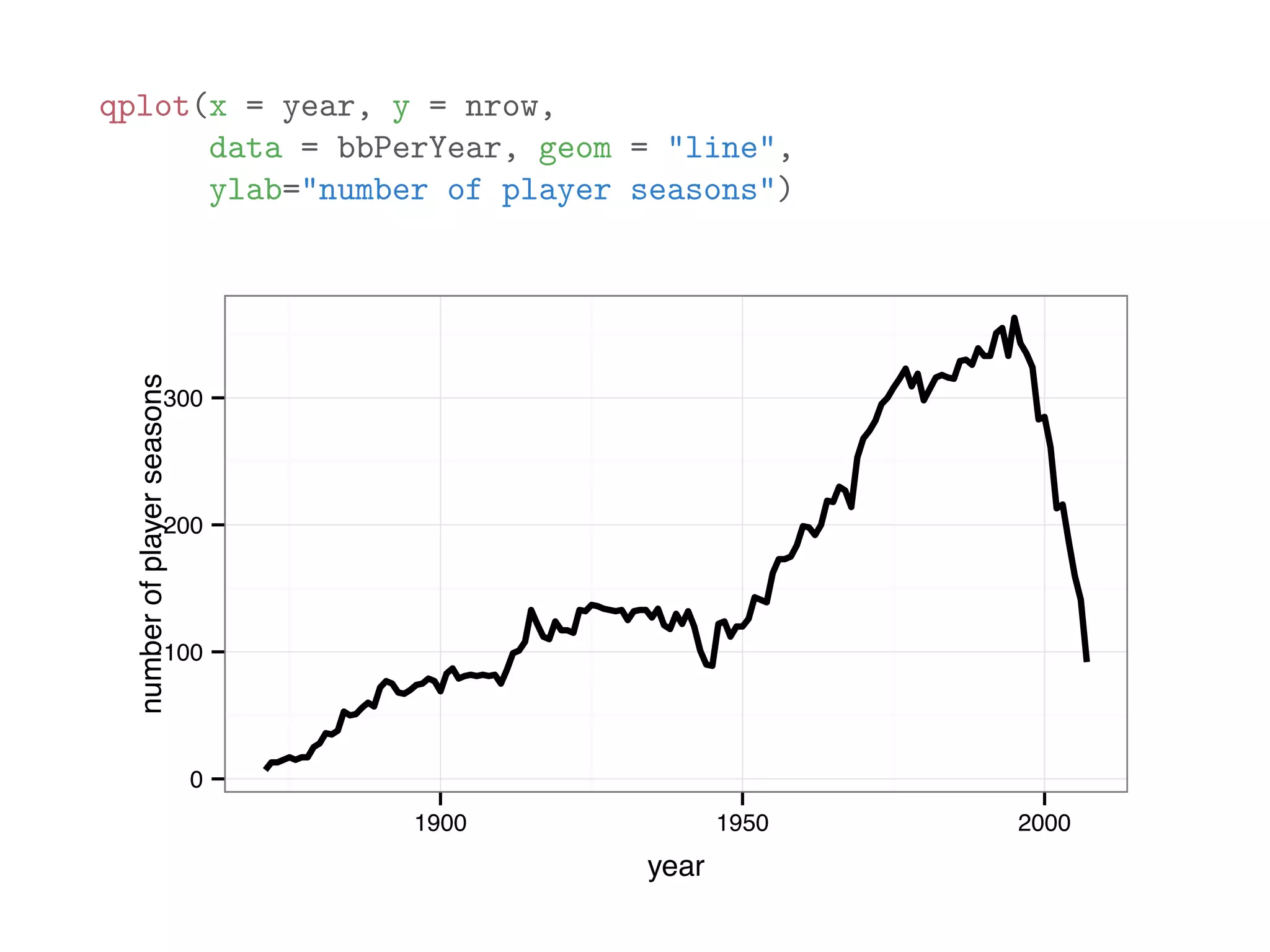
![library(plyr) names(baseball) ## [1] "id" "year" "stint" "team" "lg" "g" "ab" ## [9] "h" "X2b" "X3b" "hr" "rbi" "sb" "cs" ## [17] "so" "ibb" "hbp" "sh" "sf" "gidp" # count number of players recorded for each year bbPerYear = ddply(baseball, "year", "nrow") head(bbPerYear) ## year nrow ## 1 1871 7 ## 2 1872 13 ## 3 1873 13 ## 4 1874 15 ## 5 1875 17 ## 6 1876 15](https://image.slidesharecdn.com/rminicoursecombined-150930180229-lva1-app6891/75/Data-Analysis-with-R-combined-slides-141-2048.jpg)
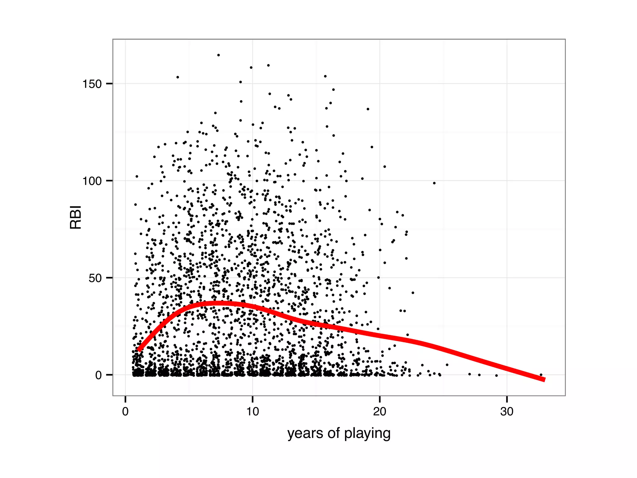
![# add a column career.year which measures the number of years # passed since each player started batting bbMod2 = ddply(baseball, "id", transform, career.year = year - min(year) + 1) # sample a random subset 3000 rows to avoid over-plotting bbSubset = bbMod2[sample(dim(bbMod2)[1], 3000),] qplot(career.year, rbi, data = bbSubset, size = I(0.8), geom = "jitter", ylab = "RBI", xlab = "years of playing") + geom_smooth(color = "red", se = F, size = 1.5)](https://image.slidesharecdn.com/rminicoursecombined-150930180229-lva1-app6891/75/Data-Analysis-with-R-combined-slides-144-2048.jpg)
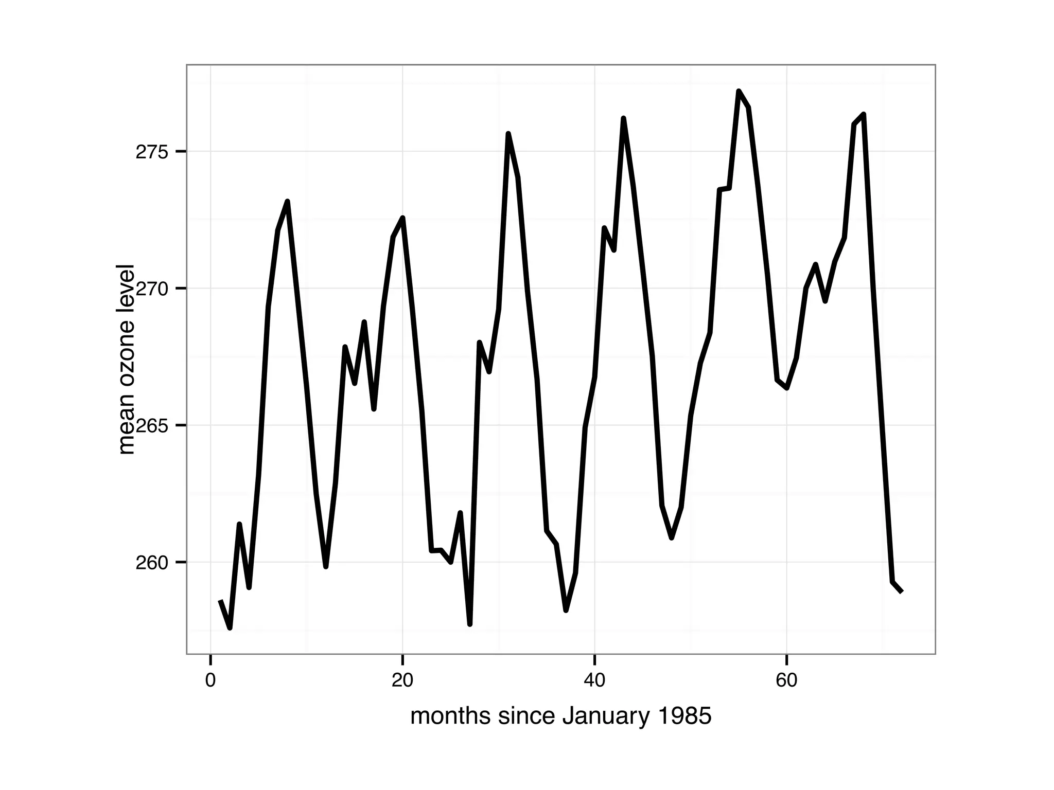

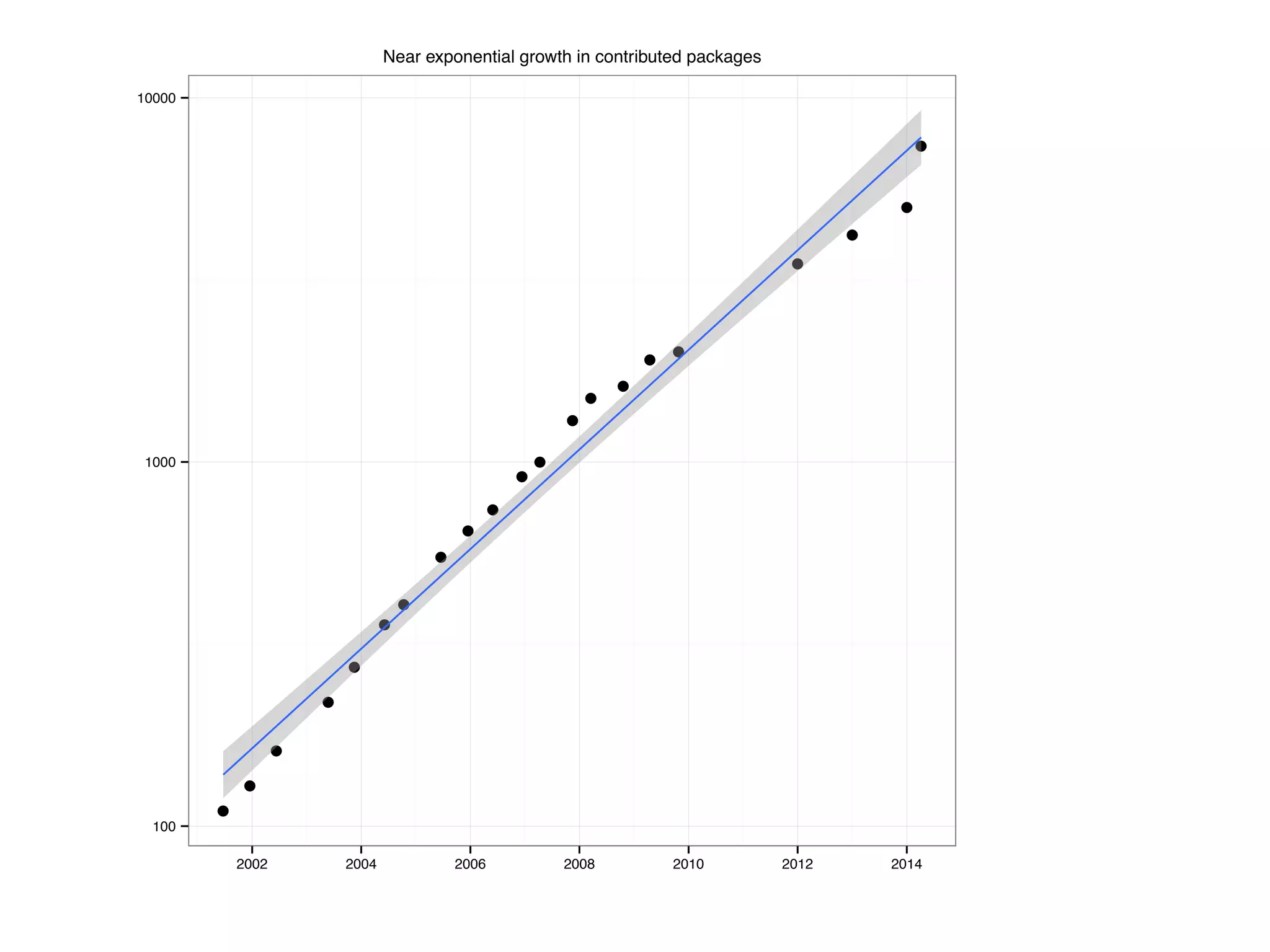
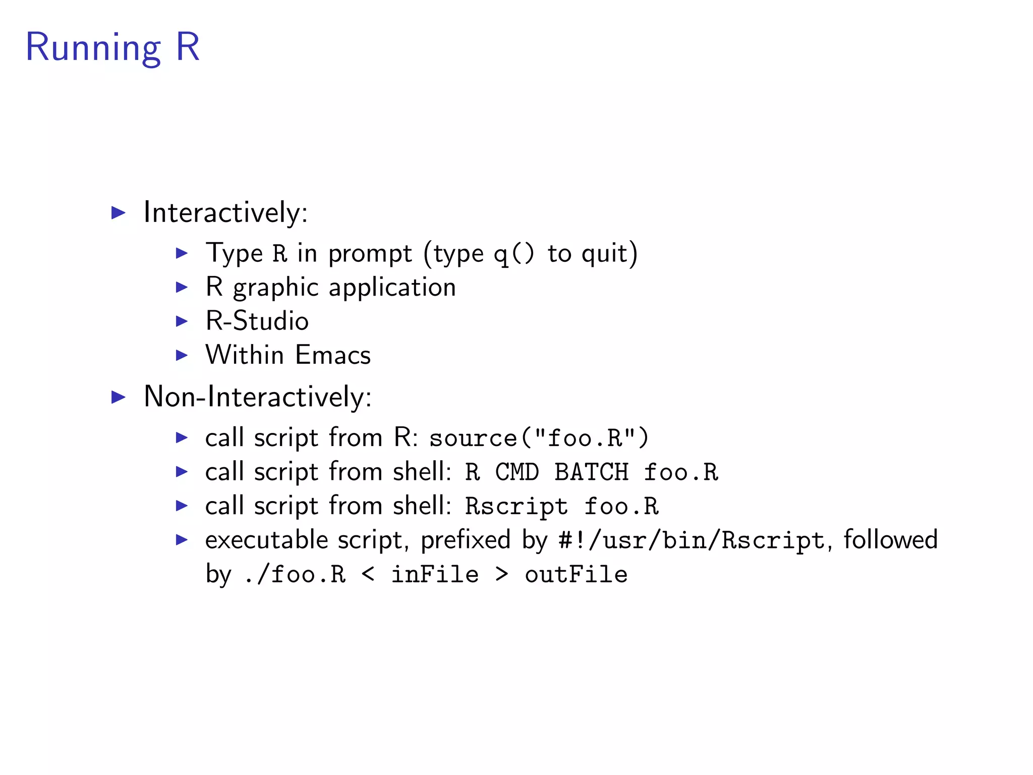
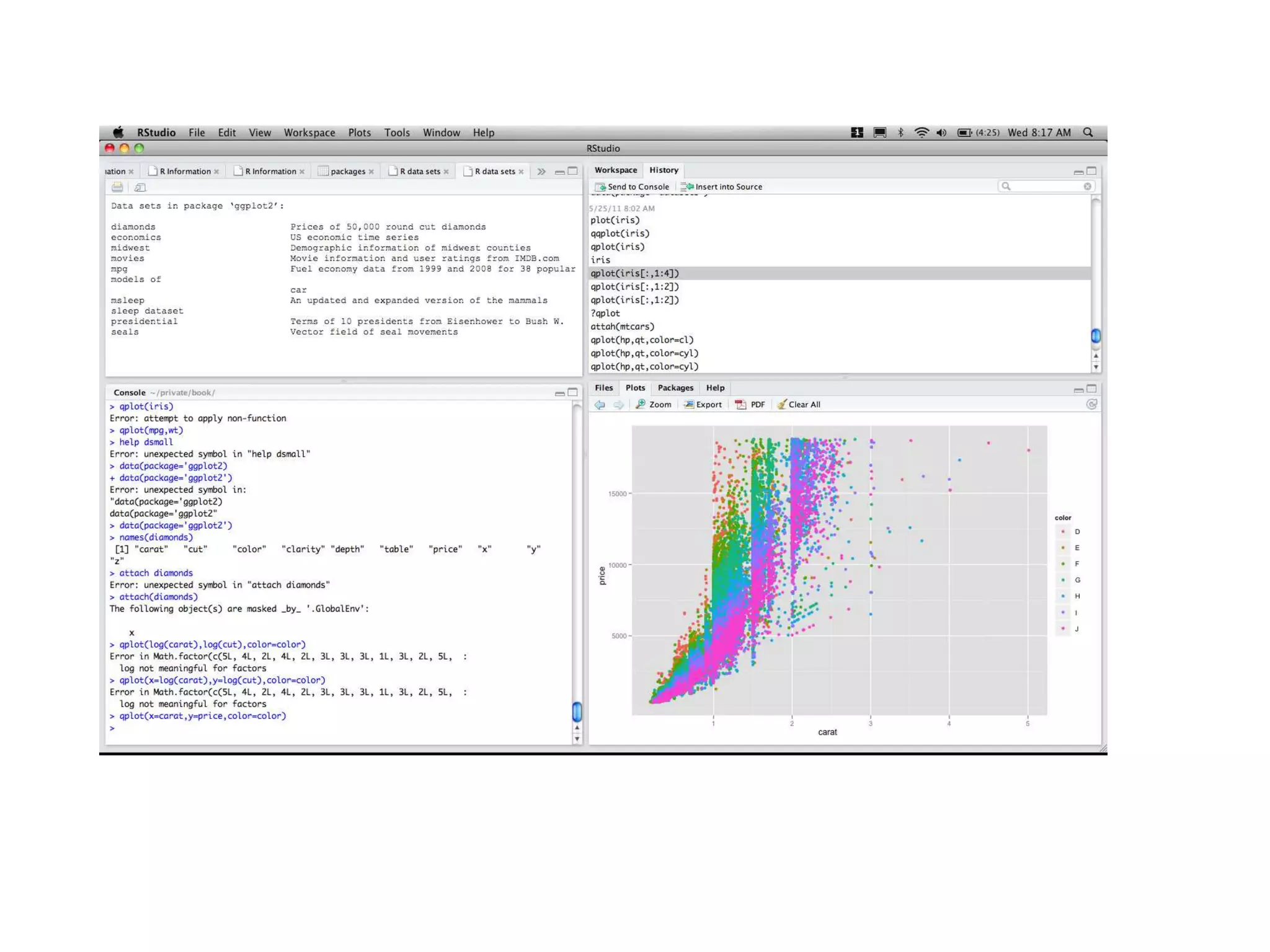
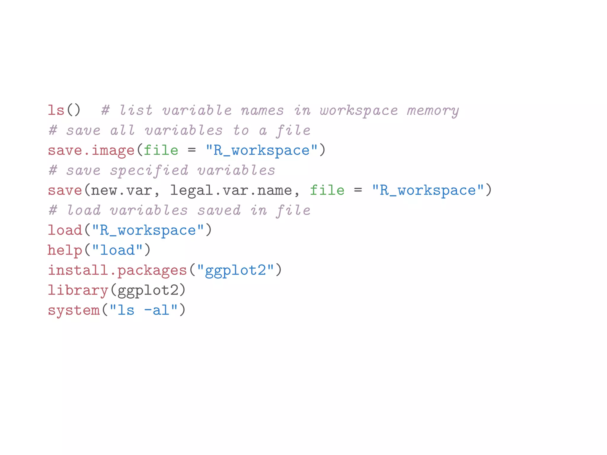
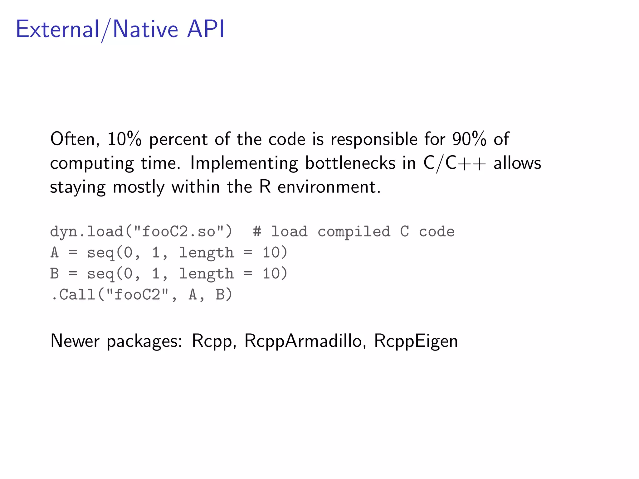
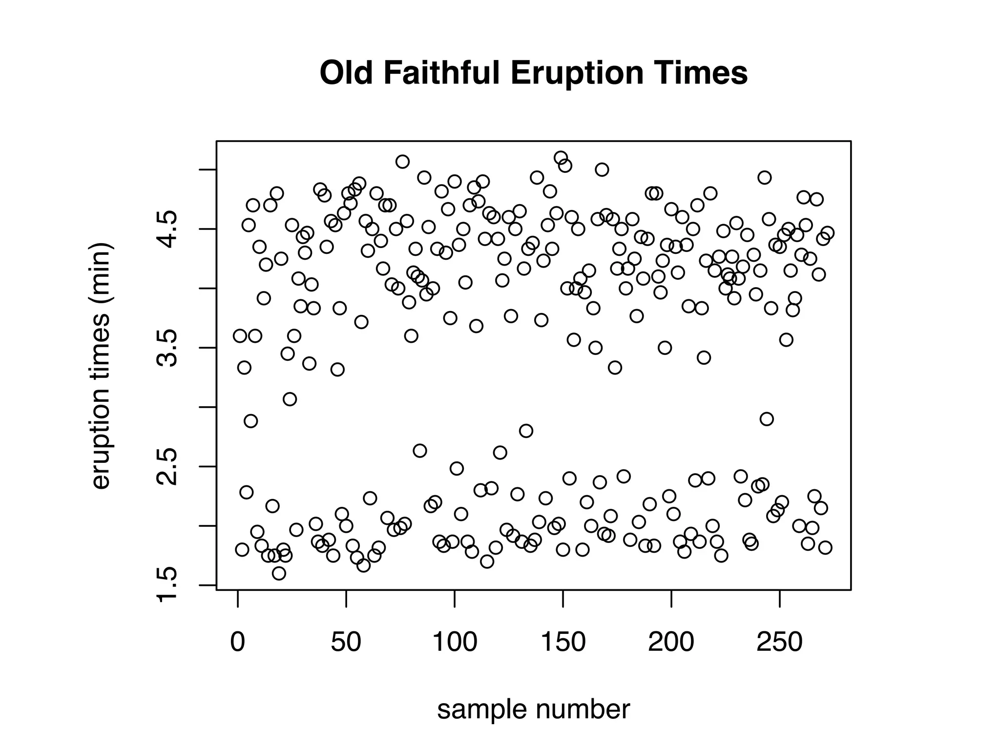
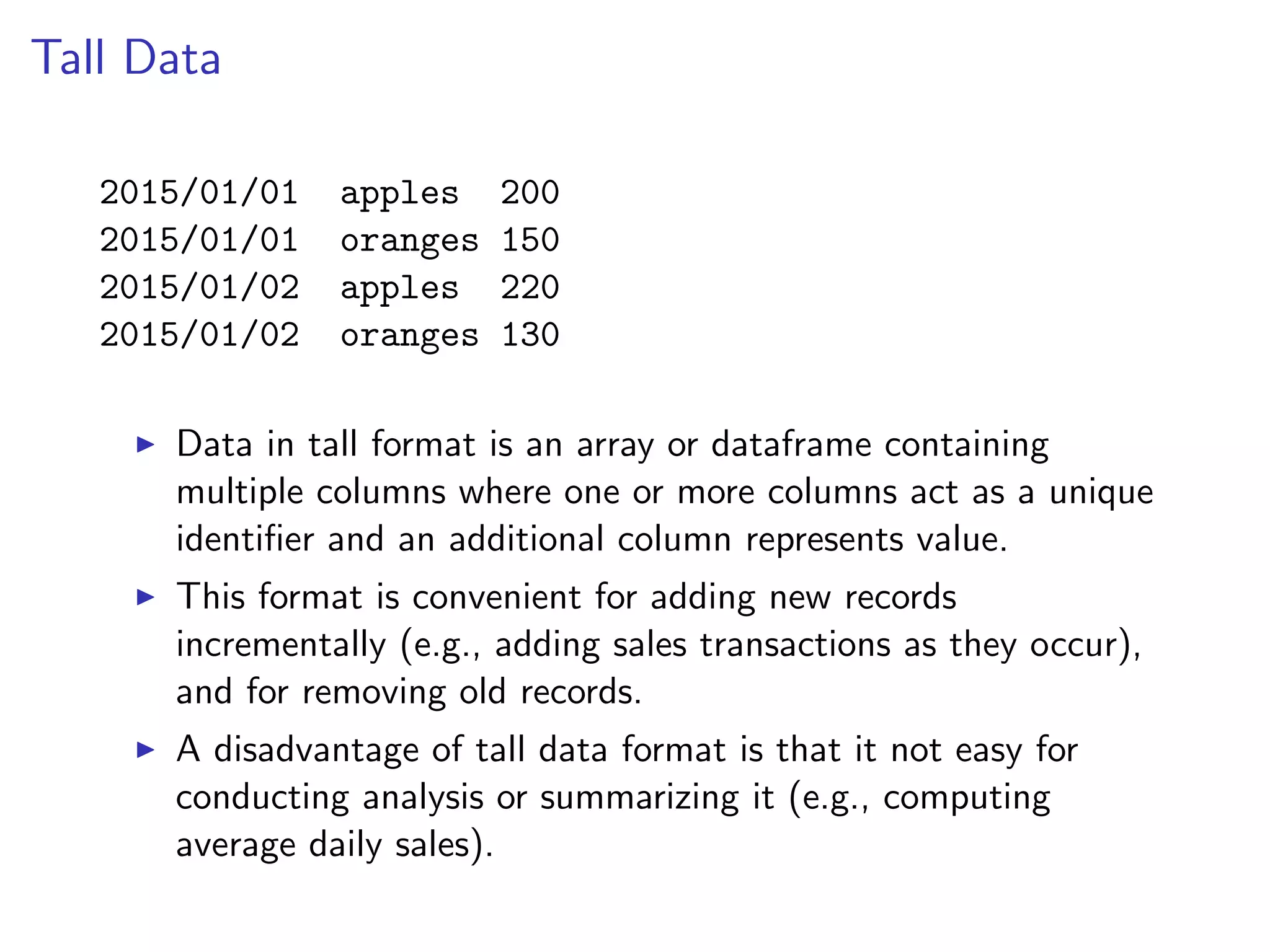
The document discusses an R programming module that will cover getting started with R, data types and structures, control flow and functions, and scalability. It compares R to MATLAB and Python, describing their similarities as interactive shells for data manipulation but noting differences in popularity across fields and open-source availability. Base graphics and ggplot2 for data visualization are introduced. Sample datasets are also mentioned.