The document provides a comprehensive guide for R developers transitioning to Python, focusing on installation, syntax differences, and data structures like vectors and data frames. It highlights the advantages of using Python 3 and the Anaconda distribution, and offers insights on libraries like NumPy for data manipulation. Key topics include vector operations, broadcasting rules, and indexing syntax in Python compared to R.


![Installation Vectors Data Frames Analysis Visualization I/O Conclusion Python syntax in 2 minutes (2) Function: # WARNING: This is purely to cover some basic python syntax # there are better ways to do this in Python def quote_pad_string(a_string): maximum_length = 10 num_missing_characters = maximum_length - len(a_string) if num_missing_characters < 0: num_missing_characters = 0 if num_missing_characters: for i in range(num_missing_characters): a_string = a_string + " " else: a_string = a_string[:maximum_length] return "’" + a_string.upper() + "’"](https://image.slidesharecdn.com/python-for-r-datascientists-160614160836/75/Python-for-R-developers-and-data-scientists-10-2048.jpg)
![Installation Vectors Data Frames Analysis Visualization I/O Conclusion Python syntax in 2 minutes (2) def defines the body of a function. Python is dynamically typed: # WARNING: This is purely to cover some basic python syntax # there are better ways to do this in Python def quote_pad_string(a_string): maximum_length = 10 num_missing_characters = maximum_length - len(a_string) if num_missing_characters < 0: num_missing_characters = 0 if num_missing_characters: for i in range(num_missing_characters): a_string = a_string + " " else: a_string = a_string[:maximum_length] return "’" + a_string.upper() + "’"](https://image.slidesharecdn.com/python-for-r-datascientists-160614160836/75/Python-for-R-developers-and-data-scientists-11-2048.jpg)
![Installation Vectors Data Frames Analysis Visualization I/O Conclusion Python syntax in 2 minutes (2) Python uses indentation for code blocks instead of curly braces: # WARNING: This is purely to cover some basic python syntax # there are better ways to do this in Python def quote_pad_string(a_string): maximum_length = 10 num_missing_characters = maximum_length - len(a_string) if num_missing_characters < 0: num_missing_characters = 0 if num_missing_characters: for i in range(num_missing_characters): a_string = a_string + " " else: a_string = a_string[:maximum_length] return "’" + a_string.upper() + "’"](https://image.slidesharecdn.com/python-for-r-datascientists-160614160836/75/Python-for-R-developers-and-data-scientists-12-2048.jpg)
![Installation Vectors Data Frames Analysis Visualization I/O Conclusion Python syntax in 2 minutes (2) ‘=’ for assignment: # WARNING: This is purely to cover some basic python syntax # there are better ways to do this in Python def quote_pad_string(a_string): maximum_length = 10 num_missing_characters = maximum_length - len(a_string) if num_missing_characters < 0: num_missing_characters = 0 if num_missing_characters: for i in range(num_missing_characters): a_string = a_string + " " else: a_string = a_string[:maximum_length] return "’" + a_string.upper() + "’"](https://image.slidesharecdn.com/python-for-r-datascientists-160614160836/75/Python-for-R-developers-and-data-scientists-13-2048.jpg)
![Installation Vectors Data Frames Analysis Visualization I/O Conclusion Python syntax in 2 minutes (2) ‘if’ statement: # WARNING: This is purely to cover some basic python syntax # there are better ways to do this in Python def quote_pad_string(a_string): maximum_length = 10 num_missing_characters = maximum_length - len(a_string) if num_missing_characters < 0: num_missing_characters = 0 if num_missing_characters: for i in range(num_missing_characters): a_string = a_string + " " else: a_string = a_string[:maximum_length] return "’" + a_string.upper() + "’"](https://image.slidesharecdn.com/python-for-r-datascientists-160614160836/75/Python-for-R-developers-and-data-scientists-14-2048.jpg)
![Installation Vectors Data Frames Analysis Visualization I/O Conclusion Python syntax in 2 minutes (2) ‘for’ statement: # WARNING: This is purely to cover some basic python syntax # there are better ways to do this in Python def quote_pad_string(a_string): maximum_length = 10 num_missing_characters = maximum_length - len(a_string) if num_missing_characters < 0: num_missing_characters = 0 if num_missing_characters: for i in range(num_missing_characters): a_string = a_string + " " else: a_string = a_string[:maximum_length] return "’" + a_string.upper() + "’"](https://image.slidesharecdn.com/python-for-r-datascientists-160614160836/75/Python-for-R-developers-and-data-scientists-15-2048.jpg)
![Installation Vectors Data Frames Analysis Visualization I/O Conclusion Python syntax in 2 minutes (2) len(a_string) is a function call, a_string.upper() is a method invocation: # WARNING: This is purely to cover some basic python syntax # there are better ways to do this in Python def quote_pad_string(a_string): maximum_length = 10 num_missing_characters = maximum_length - len(a_string) if num_missing_characters < 0: num_missing_characters = 0 if num_missing_characters: for i in range(num_missing_characters): a_string = a_string + " " else: a_string = a_string[:maximum_length] return "’" + a_string.upper() + "’"](https://image.slidesharecdn.com/python-for-r-datascientists-160614160836/75/Python-for-R-developers-and-data-scientists-16-2048.jpg)
![Installation Vectors Data Frames Analysis Visualization I/O Conclusion Scalars - R In R there are no real scalar types. They are just vectors of length 1: > a <- 5 # Equivalent to a <- c(5) > a [1] 5 > length(a) [1] 1](https://image.slidesharecdn.com/python-for-r-datascientists-160614160836/75/Python-for-R-developers-and-data-scientists-18-2048.jpg)
![Installation Vectors Data Frames Analysis Visualization I/O Conclusion Scalars - Python In Python scalars and vectors are not the same thing: >>> a = 5 # Scalar 5 >>> b = np.array([5]) # Array with one element array([5]) >>> len(b) # Equivalent to ’length’ in R 1 This won’t work: >>> len(a) TypeError: object of type ’int’ has no len()](https://image.slidesharecdn.com/python-for-r-datascientists-160614160836/75/Python-for-R-developers-and-data-scientists-19-2048.jpg)
![Installation Vectors Data Frames Analysis Visualization I/O Conclusion Vectors, matrices and arrays - R In R, there’s ‘c’ for 1d vectors, ‘matrix’ for 2 dimensions, and ‘array’ for higher-order dimensions: > c(1,2,3,4) [1] 1 2 3 4 > matrix(1:4, nrow=2,ncol=2) [,1] [,2] [1,] 1 3 [2,] 2 4 > array(1:3, c(2,4,6)) ... Strangely enough, a 1d array is not the same as a vector: > a <- as.array(1:3) [1] 1 2 3 > is.vector(a) [1] FALSE](https://image.slidesharecdn.com/python-for-r-datascientists-160614160836/75/Python-for-R-developers-and-data-scientists-20-2048.jpg)
![Installation Vectors Data Frames Analysis Visualization I/O Conclusion Vectors, matrices and arrays - Python Python has no builtin vector or matrix type. You will need numpy: >>> import numpy as np # Equivalent to ’library(numpy)’ in R. >>> np.array([1, 2, 3, 4]) # 1d vector array([1, 2, 3, 4]) >>> np.array([[1, 2], [3, 4]]) # matrix array([[1, 2], [3, 4]]) np.array works with any dimension and it’s a single type (ndarray). (There’s also a matrix type specifically for two dimensions but it should be avoided. Always use ndarray.)](https://image.slidesharecdn.com/python-for-r-datascientists-160614160836/75/Python-for-R-developers-and-data-scientists-21-2048.jpg)
![Installation Vectors Data Frames Analysis Visualization I/O Conclusion Generating regular sequences R > 5:10 # Shortend for seq [1] 5 6 7 8 9 10 > seq(0, 1, length.out = 11) [1] 0.0 0.1 0.2 0.3 0.4 0.5 0.6 0.7 0.8 0.9 1.0 Python >>> np.arange(3.0) array([ 0., 1., 2.]) >>> np.arange(3, 7) array([3, 4, 5, 6]) >>> np.arange(3, 7, 2) array([3, 5])](https://image.slidesharecdn.com/python-for-r-datascientists-160614160836/75/Python-for-R-developers-and-data-scientists-22-2048.jpg)
![Installation Vectors Data Frames Analysis Visualization I/O Conclusion Vector operations - Python For the most part, vector operations in Python work just like in R: >>> a = np.arange(5.0) array([ 0., 1., 2., 3., 4.]) >>> 1.0 + a # Adding array([ 1., 2., 3., 4., 5.]) >>> a * a # Multiplying element wise array([ 0., 1., 4., 9., 16.]) >>> a ** 3 # to the power of 3 array([ 0., 1., 8., 27., 64.])](https://image.slidesharecdn.com/python-for-r-datascientists-160614160836/75/Python-for-R-developers-and-data-scientists-23-2048.jpg)
![Installation Vectors Data Frames Analysis Visualization I/O Conclusion Vector operations - Python (2) For matrix multiplication use the ‘@’ operator: >> a = np.array([[1, 0], [0, 1]]) array([[1, 0], [0, 1]]) >> b = np.array([[4, 1], [2, 2]]) array([[4, 1], [2, 2]]) >> a @ b array([[4, 1], [2, 2]]) (In Python 2 use np.dot(a,b).)](https://image.slidesharecdn.com/python-for-r-datascientists-160614160836/75/Python-for-R-developers-and-data-scientists-24-2048.jpg)
![Installation Vectors Data Frames Analysis Visualization I/O Conclusion Vector operations - Python (3) Numpy also has the usual mathematical operations that work on vectors: >> a = np.arange(5.0) array([ 0., 1., 2., 3., 4.]) >> np.sin(a) array([ 0., 0.84147098, 0.90929743, 0.14112001, -0.7568025 ]) Full reference here: http://docs.scipy.org/doc/numpy/reference/routines.math.html](https://image.slidesharecdn.com/python-for-r-datascientists-160614160836/75/Python-for-R-developers-and-data-scientists-25-2048.jpg)
![Installation Vectors Data Frames Analysis Visualization I/O Conclusion Recycling - R When doing vector operations, R automatically extends the smallest element to be as large as the other: > c(1,2) + c(1,2,3,4) # Equivalent to c(1,2,1,2) + c(1,2,3,4) [1] 2 4 4 6 You can do this even if the lengths aren’t multiples of one another, albeit with a warning: > c(1,2) + c(1,2,3,4,5) [1] 2 4 4 6 6 Warning message: In c(1, 2) + c(1,2,3,4,5) : longer object length is not a multiple of shorter object length](https://image.slidesharecdn.com/python-for-r-datascientists-160614160836/75/Python-for-R-developers-and-data-scientists-26-2048.jpg)


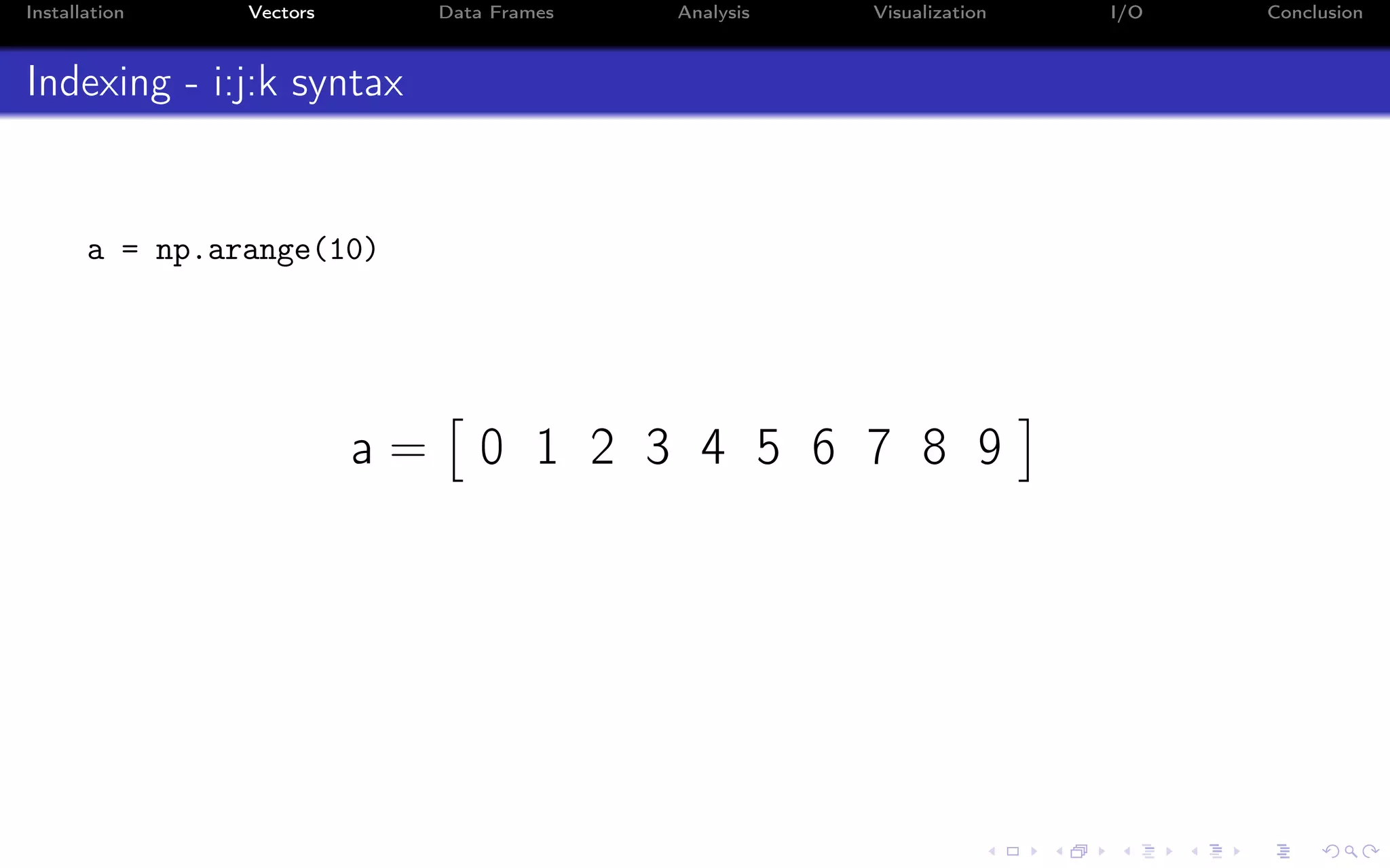
![Installation Vectors Data Frames Analysis Visualization I/O Conclusion Indexing - i:j:k syntax a = np.arange(10) a = 0 1 2 3 4 5 6 7 8 9 Indexing in Python starts from 0 (not 1): >>> a[0] 0.0 Indexing on a single value returns a scalar (not an array!)](https://image.slidesharecdn.com/python-for-r-datascientists-160614160836/75/Python-for-R-developers-and-data-scientists-36-2048.jpg)
![Installation Vectors Data Frames Analysis Visualization I/O Conclusion Indexing - i:j:k syntax a = np.arange(10) a = 0 1 2 3 4 5 6 7 8 9 Use ‘i:j’ to index from position i to j-1: >>> a[1:3] array([ 1, 2])](https://image.slidesharecdn.com/python-for-r-datascientists-160614160836/75/Python-for-R-developers-and-data-scientists-37-2048.jpg)
![Installation Vectors Data Frames Analysis Visualization I/O Conclusion Indexing - i:j:k syntax a = np.arange(10) a = 0 1 2 3 4 5 6 7 8 9 An optional ‘k’ element defines the step: >>> a[1:7:2] array([1, 3, 5])](https://image.slidesharecdn.com/python-for-r-datascientists-160614160836/75/Python-for-R-developers-and-data-scientists-38-2048.jpg)
![Installation Vectors Data Frames Analysis Visualization I/O Conclusion Indexing - i:j:k syntax a = np.arange(10) a = 0 1 2 3 4 5 6 7 8 9 i and j can be negative, which means they will start counting from the last: >>> a[1:-3] array([1, 2, 3, 4, 5, 6])](https://image.slidesharecdn.com/python-for-r-datascientists-160614160836/75/Python-for-R-developers-and-data-scientists-39-2048.jpg)
![Installation Vectors Data Frames Analysis Visualization I/O Conclusion Indexing - i:j:k syntax a = np.arange(10) a = 0 1 2 3 4 5 6 7 8 9 i and j can be negative, which means they will start counting from the last: >>> a[-3:-1] array([7, 8])](https://image.slidesharecdn.com/python-for-r-datascientists-160614160836/75/Python-for-R-developers-and-data-scientists-40-2048.jpg)
![Installation Vectors Data Frames Analysis Visualization I/O Conclusion Indexing - i:j:k syntax a = np.arange(10) a = 0 1 2 3 4 5 6 7 8 9 While a negative k will go in the opposite direction: >>> a[-3:-9:-1] array([7, 6, 5, 4, 3, 2])](https://image.slidesharecdn.com/python-for-r-datascientists-160614160836/75/Python-for-R-developers-and-data-scientists-41-2048.jpg)
![Installation Vectors Data Frames Analysis Visualization I/O Conclusion Indexing - i:j:k syntax a = np.arange(10) a = 0 1 2 3 4 5 6 7 8 9 Not all need to be included: >>> a[::-1] array([9, 8, 7, 6, 5, 4, 3, 2, 1, 0])](https://image.slidesharecdn.com/python-for-r-datascientists-160614160836/75/Python-for-R-developers-and-data-scientists-42-2048.jpg)
![Installation Vectors Data Frames Analysis Visualization I/O Conclusion Indexing - multiple dimensions Use ‘,’ for additional dimensions: x = 1 2 3 4 5 6 >>> x[0:2, 0:1] array([[1], [4]])](https://image.slidesharecdn.com/python-for-r-datascientists-160614160836/75/Python-for-R-developers-and-data-scientists-43-2048.jpg)
![Installation Vectors Data Frames Analysis Visualization I/O Conclusion Indexing using conditions Operators like ‘>’ or ‘<=’ operate element-wise and return a logical vector: >>> a > 4 array([False, False, False, False, False, True, True, True, True, True], dtype=bool) These can be combined into more complex expressions: >> (a > 2) && (b ** 2 <= a) ... And used as indexing too: >> a[a > 4] array([5, 6, 7, 8, 9])](https://image.slidesharecdn.com/python-for-r-datascientists-160614160836/75/Python-for-R-developers-and-data-scientists-44-2048.jpg)
![Installation Vectors Data Frames Analysis Visualization I/O Conclusion Assignment Any index can be used together with ‘=’ for assignment: >>> a[0] = 10 array([10, 1, 2, 3, 4, 5, 6, 7, 8, 9]) Conditions work as well: >>> a[a > 4] = 99 array([99, 1, 2, 3, 4, 99, 99, 99, 99, 99])](https://image.slidesharecdn.com/python-for-r-datascientists-160614160836/75/Python-for-R-developers-and-data-scientists-45-2048.jpg)


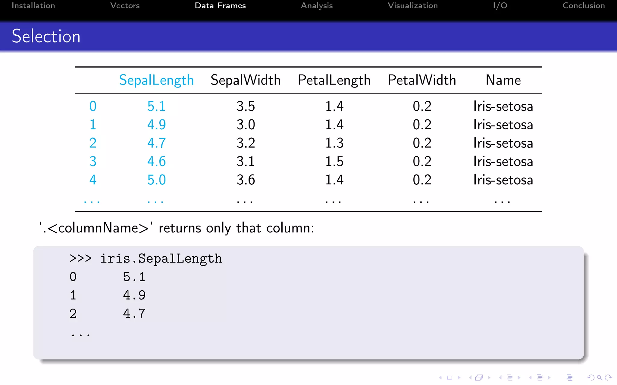
![Installation Vectors Data Frames Analysis Visualization I/O Conclusion Selection SepalLength SepalWidth PetalLength PetalWidth Name 0 5.1 3.5 1.4 0.2 Iris-setosa 1 4.9 3.0 1.4 0.2 Iris-setosa 2 4.7 3.2 1.3 0.2 Iris-setosa 3 4.6 3.1 1.5 0.2 Iris-setosa 4 5.0 3.6 1.4 0.2 Iris-setosa . . . . . . . . . . . . . . . . . . This also works: >>> iris["SepalLength"] ...](https://image.slidesharecdn.com/python-for-r-datascientists-160614160836/75/Python-for-R-developers-and-data-scientists-50-2048.jpg)
![Installation Vectors Data Frames Analysis Visualization I/O Conclusion Selection SepalLength SepalWidth PetalLength PetalWidth Name 0 5.1 3.5 1.4 0.2 Iris-setosa 1 4.9 3.0 1.4 0.2 Iris-setosa 2 4.7 3.2 1.3 0.2 Iris-setosa 3 4.6 3.1 1.5 0.2 Iris-setosa 4 5.0 3.6 1.4 0.2 Iris-setosa . . . . . . . . . . . . . . . . . . You can select multiple columns by passing a list: >>> iris[["SepalWidth", "SepalLength"]] SepalWidth SepalLength 0 3.5 5.1 1 3.0 4.9 ...](https://image.slidesharecdn.com/python-for-r-datascientists-160614160836/75/Python-for-R-developers-and-data-scientists-51-2048.jpg)
![Installation Vectors Data Frames Analysis Visualization I/O Conclusion Selection SepalLength SepalWidth PetalLength PetalWidth Name 0 5.1 3.5 1.4 0.2 Iris-setosa 1 4.9 3.0 1.4 0.2 Iris-setosa 2 4.7 3.2 1.3 0.2 Iris-setosa 3 4.6 3.1 1.5 0.2 Iris-setosa 4 5.0 3.6 1.4 0.2 Iris-setosa . . . . . . . . . . . . . . . . . . Or if you pass a slice you can select rows: >>> iris[1:3] SepalLength SepalWidth PetalLength PetalWidth Name 1 4.9 3.0 1.4 0.2 Iris-setosa 2 4.7 3.2 1.3 0.2 Iris-setosa](https://image.slidesharecdn.com/python-for-r-datascientists-160614160836/75/Python-for-R-developers-and-data-scientists-52-2048.jpg)
![Installation Vectors Data Frames Analysis Visualization I/O Conclusion Selection SepalLength SepalWidth PetalLength PetalWidth Name 0 5.1 3.5 1.4 0.2 Iris-setosa 1 4.9 3.0 1.4 0.2 Iris-setosa 2 4.7 3.2 1.3 0.2 Iris-setosa 3 4.6 3.1 1.5 0.2 Iris-setosa 4 5.0 3.6 1.4 0.2 Iris-setosa . . . . . . . . . . . . . . . . . . With loc you can slice both rows and columns: >>> iris.loc[1:3, ["SepalLength", "SepalWidth"]] SepalLength SepalWidth 1 4.9 3.0 2 4.7 3.2 3 4.6 3.1 loc is inclusive at the end.](https://image.slidesharecdn.com/python-for-r-datascientists-160614160836/75/Python-for-R-developers-and-data-scientists-53-2048.jpg)
![Installation Vectors Data Frames Analysis Visualization I/O Conclusion Selection SepalLength SepalWidth PetalLength PetalWidth Name 0 5.1 3.5 1.4 0.2 Iris-setosa 1 4.9 3.0 1.4 0.2 Iris-setosa 2 4.7 3.2 1.3 0.2 Iris-setosa 3 4.6 3.1 1.5 0.2 Iris-setosa 4 5.0 3.6 1.4 0.2 Iris-setosa . . . . . . . . . . . . . . . . . . As well as only one single row: >>> iris.loc[3] SepalLength 4.6 SepalWidth 3.1 PetalLength 1.5 PetalWidth 0.2 Name Iris-setosa Name: 3, dtype: object](https://image.slidesharecdn.com/python-for-r-datascientists-160614160836/75/Python-for-R-developers-and-data-scientists-54-2048.jpg)
![Installation Vectors Data Frames Analysis Visualization I/O Conclusion Selection SepalLength SepalWidth PetalLength PetalWidth Name 0 5.1 3.5 1.4 0.2 Iris-setosa 1 4.9 3.0 1.4 0.2 Iris-setosa 2 4.7 3.2 1.3 0.2 Iris-setosa 3 4.6 3.1 1.5 0.2 Iris-setosa 4 5.0 3.6 1.4 0.2 Iris-setosa . . . . . . . . . . . . . . . . . . iloc works with integer indices, similar to numpy arrays: >>> iris.iloc[0:2, 0:3] SepalLength SepalWidth PetalLength 0 5.1 3.5 1.4 1 4.9 3.0 1.4](https://image.slidesharecdn.com/python-for-r-datascientists-160614160836/75/Python-for-R-developers-and-data-scientists-55-2048.jpg)
![Installation Vectors Data Frames Analysis Visualization I/O Conclusion Selection SepalLength SepalWidth PetalLength PetalWidth Name 0 5.1 3.5 1.4 0.2 Iris-setosa 1 4.9 3.0 1.4 0.2 Iris-setosa 2 4.7 3.2 1.3 0.2 Iris-setosa 3 4.6 3.1 1.5 0.2 Iris-setosa 4 5.0 3.6 1.4 0.2 Iris-setosa . . . . . . . . . . . . . . . . . . ‘:’ will include all the rows (or all the columns): >>> iris.iloc[0:2, :] SepalLength SepalWidth PetalLength PetalWidth Name 0 5.1 3.5 1.4 0.2 Iris-setosa 1 4.9 3.0 1.4 0.2 Iris-setosa](https://image.slidesharecdn.com/python-for-r-datascientists-160614160836/75/Python-for-R-developers-and-data-scientists-56-2048.jpg)
![Installation Vectors Data Frames Analysis Visualization I/O Conclusion Selection SepalLength SepalWidth PetalLength PetalWidth Name 0 5.1 3.5 1.4 0.2 Iris-setosa 1 4.9 3.0 1.4 0.2 Iris-setosa 2 4.7 3.2 1.3 0.2 Iris-setosa 3 4.6 3.1 1.5 0.2 Iris-setosa 4 5.0 3.6 1.4 0.2 Iris-setosa . . . . . . . . . . . . . . . . . . Or you can use conditions like numpy: >>> iris[iris.SepalLength < 5] SepalLength SepalWidth PetalLength PetalWidth Name 1 4.9 3.0 1.4 0.2 Iris-setosa 2 4.7 3.2 1.3 0.2 Iris-setosa 3 4.6 3.1 1.5 0.2 Iris-setosa ...](https://image.slidesharecdn.com/python-for-r-datascientists-160614160836/75/Python-for-R-developers-and-data-scientists-57-2048.jpg)
![Installation Vectors Data Frames Analysis Visualization I/O Conclusion Selection SepalLength SepalWidth PetalLength PetalWidth Name 0 5.1 3.5 1.4 0.2 Iris-setosa 1 4.9 3.0 1.4 0.2 Iris-setosa 2 4.7 3.2 1.3 0.2 Iris-setosa 3 4.6 3.1 1.5 0.2 Iris-setosa 4 5.0 3.6 1.4 0.2 Iris-setosa . . . . . . . . . . . . . . . . . . Picking a single value returns a scalar: >>> iris.iloc[0,0] 5.0999999999999996 Normally it’s better to use at or iat (faster).](https://image.slidesharecdn.com/python-for-r-datascientists-160614160836/75/Python-for-R-developers-and-data-scientists-58-2048.jpg)
![Installation Vectors Data Frames Analysis Visualization I/O Conclusion Assignment Assignment works as expected: >>> iris.loc[iris.SepalLength > 7.6, "Name"] = "Iris-orlando" Beware that this doesn’t work: >> iris[iris.SepalLength > 7.6].Name = "Iris-orlando" SettingWithCopyWarning: A value is trying to be set on a copy of a slice from a DataFrame.](https://image.slidesharecdn.com/python-for-r-datascientists-160614160836/75/Python-for-R-developers-and-data-scientists-59-2048.jpg)
![Installation Vectors Data Frames Analysis Visualization I/O Conclusion Operations Operators work as expected: >>> iris["SepalD"] = iris["SepalLength"] * iris["SepalWidth"] There’s also apply: >>> iris[["SepalLength", "SepalWidth"]].apply(np.sqrt) SepalLength SepalWidth 0 2.258318 1.870829 1 2.213594 1.732051 ... Use axis=1 to apply function to each row.](https://image.slidesharecdn.com/python-for-r-datascientists-160614160836/75/Python-for-R-developers-and-data-scientists-60-2048.jpg)

![Installation Vectors Data Frames Analysis Visualization I/O Conclusion Time Series (2) Use loc to select based on dates: >>> aapl.loc[’20130131’:’20130217’] Open High Low Close Volume Date 2013-01-31 65.28 65.61 65.00 65.07 79833215 2013-02-01 65.59 65.64 64.05 64.80 134867089 ... Use iloc as before for selecting based on numerical indices: >>> aapl.iloc[1:3] Open High Low Close Volume Date 2013-01-03 78.27 78.52 77.29 77.44 88240950 2013-01-04 76.71 76.95 75.12 75.29 148581860](https://image.slidesharecdn.com/python-for-r-datascientists-160614160836/75/Python-for-R-developers-and-data-scientists-64-2048.jpg)
![Installation Vectors Data Frames Analysis Visualization I/O Conclusion Statistical tests Use scipy.stats for common statistical tests: >>> from scipy import stats >>> iris_virginica = iris[iris.Name == ’Iris-virginica’].SepalLength.values >>> iris_setosa = iris[iris.Name == ’Iris-setosa’].SepalLength.values >>> t_test = stats.ttest_ind(iris_virginica, iris_setosa) >>> t_test.pvalue 6.8925460606740589e-28 Use scikits.bootstrap for bootstrapped confidence intervals.](https://image.slidesharecdn.com/python-for-r-datascientists-160614160836/75/Python-for-R-developers-and-data-scientists-66-2048.jpg)
![Installation Vectors Data Frames Analysis Visualization I/O Conclusion Decision trees Use scikit-learn: >>> from sklearn import tree >>> clf = tree.DecisionTreeClassifier() >>> clf = clf.fit(sk_iris.data, sk_iris.target) After being fitted, the model can then be used to predict the class of samples: >>> clf.predict([[5.1, 3.5, 1.4, 0.2]]) array([0])](https://image.slidesharecdn.com/python-for-r-datascientists-160614160836/75/Python-for-R-developers-and-data-scientists-69-2048.jpg)
![Installation Vectors Data Frames Analysis Visualization I/O Conclusion Support Vector Machines scikit-learn has a very regular API. Here’s the same example using an SVM: >>> from sklearn import svm >>> clf_svm = svm.SVC() >>> clf_svm = clf_svm.fit(sk_iris.data, sk_iris.target) >>> clf_svm.predict([[5.1, 3.5, 1.4, 0.2]]) array([0])](https://image.slidesharecdn.com/python-for-r-datascientists-160614160836/75/Python-for-R-developers-and-data-scientists-70-2048.jpg)
![Installation Vectors Data Frames Analysis Visualization I/O Conclusion Principal Component Analysis from sklearn import decomposition pca = decomposition.PCA(n_components=3) pca = pca.fit(sk_iris.data) explained_variance_ratio_ and components_ will include the explained variance and the PCA components respectively: >>> pca.explained_variance_ratio_ array([ 0.92461621, 0.05301557, 0.01718514]) >>>pca.components_ array([[ 0.36158968, -0.08226889, 0.85657211, 0.35884393], [-0.65653988, -0.72971237, 0.1757674 , 0.07470647], [ 0.58099728, -0.59641809, -0.07252408, -0.54906091]])](https://image.slidesharecdn.com/python-for-r-datascientists-160614160836/75/Python-for-R-developers-and-data-scientists-72-2048.jpg)

![Installation Vectors Data Frames Analysis Visualization I/O Conclusion NAs There’s no builtin NA in Python. You normally use NaN for NAs. numpy has a bunch of builtin functions to ignore NaNs: >>> a = np.array([1.0, 3.0, np.NaN, 5.0]) >>> a.sum() nan >>> np.nansum(a) 9.0 Pandas usually ignores NaNs when computing sums, means, etc.. but propagates them accordingly. scikit-learn assumes there’s no missing data so be sure to pre-process them, e.g. remove them or set them to 0. Look at sklearn.preprocessing.Imputer statsmodels also use NaNs for missing data, but only has basic support for handling them (it can only ignore them or raise an error). See the missing attribute in the model class.](https://image.slidesharecdn.com/python-for-r-datascientists-160614160836/75/Python-for-R-developers-and-data-scientists-74-2048.jpg)
![Installation Vectors Data Frames Analysis Visualization I/O Conclusion Pandas read_csv Reads data from CSV files >>> pd.read_csv(’foo.csv’) Unnamed: 0 A B C D 0 2000-01-01 0.266457 -0.399641 -0.219582 1.186860 1 2000-01-02 -1.170732 -0.345873 1.653061 -0.282953 ... Conversely there is to_csv to write CSV files: In [136]: df.to_csv(’foo.csv’)](https://image.slidesharecdn.com/python-for-r-datascientists-160614160836/75/Python-for-R-developers-and-data-scientists-80-2048.jpg)

![Installation Vectors Data Frames Analysis Visualization I/O Conclusion h5py - datasets Creating a data set: >>> import h5py >>> import numpy as np >>> >>> f = h5py.File("mytestfile.hdf5", "w") >>> dset = f.create_dataset("mydataset", (100,), dtype=’i’) Datasets work similarly to numpy arrays: >>> dset[...] = np.arange(100) >>> dset[0] 0 >>> dset[10] 10 >>> dset[0:100:10] array([ 0, 10, 20, 30, 40, 50, 60, 70, 80, 90])](https://image.slidesharecdn.com/python-for-r-datascientists-160614160836/75/Python-for-R-developers-and-data-scientists-82-2048.jpg)