Download to read offline


![# Read data trainingSet <- read.csv(trainingFile, header = FALSE) testSet <- read.csv(testFile, header = FALSE) trainingSet$V65 <- factor(trainingSet$V65) testSet$V65 <- factor(testSet$V65) # Classify library(caret) knn.fit <- knn3(V65 ~ ., data=trainingSet, k=5) # Predict new values pred.test <- predict(knn.fit, testSet[,1:64], type="class")](https://image.slidesharecdn.com/rmachinelearning-170523094935/75/Clean-Learn-and-Visualise-data-with-R-18-2048.jpg)
![# Confusion matrix library(caret) confusionMatrix(pred.test, testSet[,65])](https://image.slidesharecdn.com/rmachinelearning-170523094935/75/Clean-Learn-and-Visualise-data-with-R-19-2048.jpg)
![# Pairs for the numeric data pairs(Prestige[,-c(5,6)], pch=21, bg=Prestige$type)](https://image.slidesharecdn.com/rmachinelearning-170523094935/75/Clean-Learn-and-Visualise-data-with-R-24-2048.jpg)
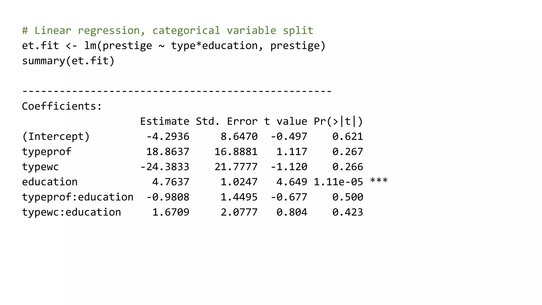
![# Pairs for the numeric data cf <- et.fit$coefficients ggplot(prestige, aes(education, prestige)) + geom_point(aes(col=type)) + geom_abline(slope=cf[4], intercept = cf[1], colour='red') + geom_abline(slope=cf[4] + cf[5], intercept = cf[1] + cf[2], colour='green') + geom_abline(slope=cf[4] + cf[6], intercept = cf[1] + cf[3], colour='blue')](https://image.slidesharecdn.com/rmachinelearning-170523094935/75/Clean-Learn-and-Visualise-data-with-R-30-2048.jpg)
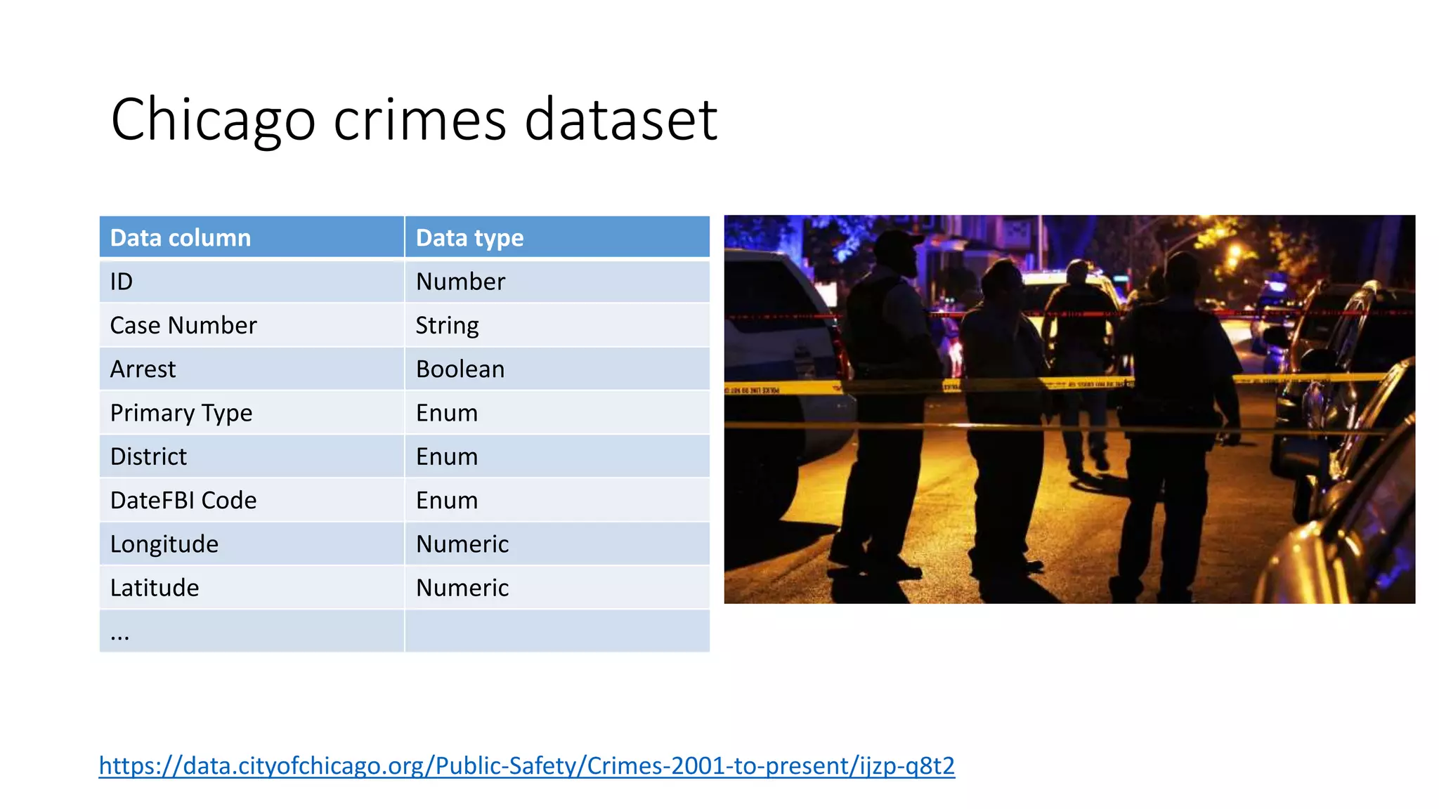
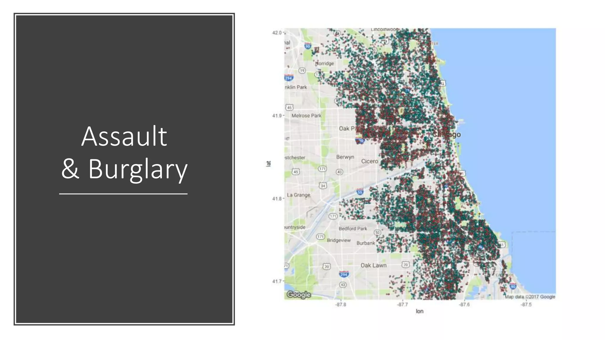
![# Read data crimeData <- read.csv(crimeFilePath) # Only data with location, only Assault or Burglary types crimeData <- crimeData[ !is.na(crimeData$Latitude) & !is.na(crimeData$Longitude),] selectedCrimes <- subset(crimeData, Primary.Type %in% c(crimeTypes[2], crimeTypes[4])) # Visualise library(ggplot2) library(ggmap) # Get map from Google map_g <- get_map(location=c(lon=mean(crimeData$Longitude, na.rm=TRUE), lat=mean( crimeData$Latitude, na.rm=TRUE)), zoom = 11, maptype = "terrain", scale = 2) ggmap(map_g) + geom_point(data = selectedCrimes, aes(x = Longitude, y = Latitude, fill = Primary.Type, alpha = 0.8), size = 1, shape = 21) + guides(fill=FALSE, alpha=FALSE, size=FALSE)](https://image.slidesharecdn.com/rmachinelearning-170523094935/75/Clean-Learn-and-Visualise-data-with-R-34-2048.jpg)
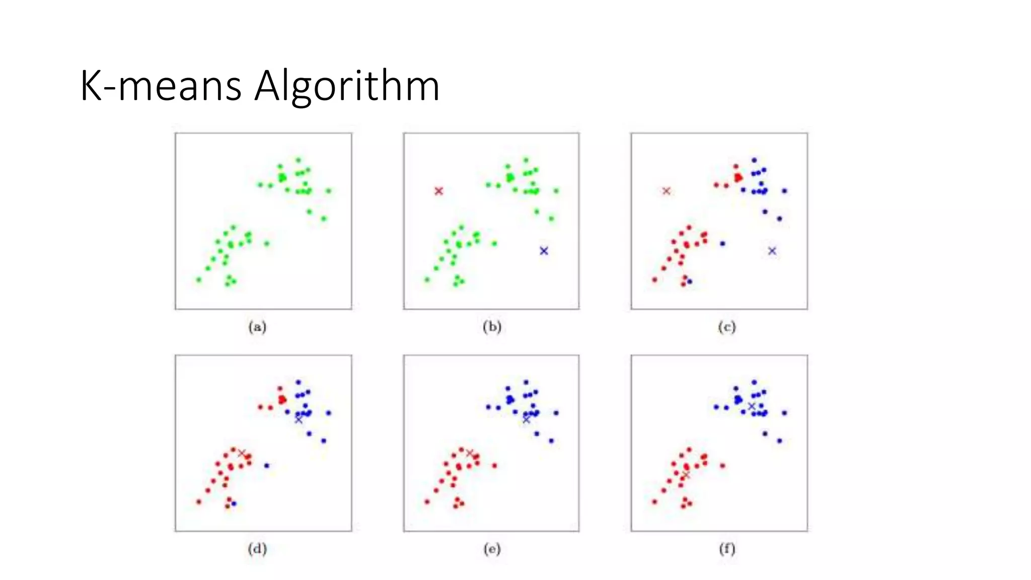
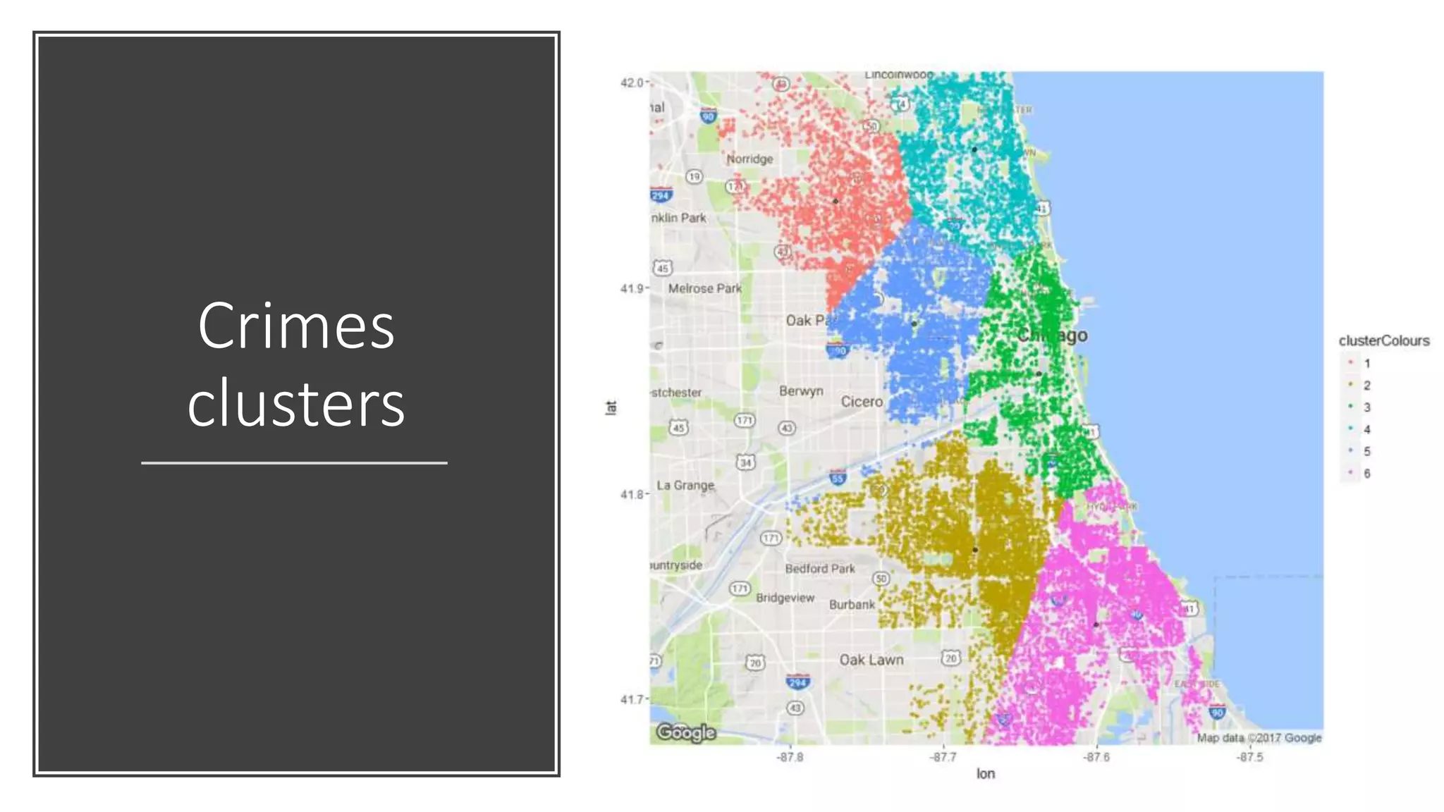
![# k-means clustering (k=6) clusterResult <- kmeans(selectedCrimes[, c('Longitude', 'Latitude')], 6) # Get the clusters information centers <- as.data.frame(clusterResult$centers) clusterColours <- factor(clusterResult$cluster) # Visualise ggmap(map_g) + geom_point(data = selectedCrimes, aes(x = Longitude, y = Latitude, alpha = 0.8, color = clusterColours), size = 1) + geom_point(data = centers, aes(x = Longitude, y = Latitude, alpha = 0.8), size = 1.5) + guides(fill=FALSE, alpha=FALSE, size=FALSE)](https://image.slidesharecdn.com/rmachinelearning-170523094935/75/Clean-Learn-and-Visualise-data-with-R-36-2048.jpg)
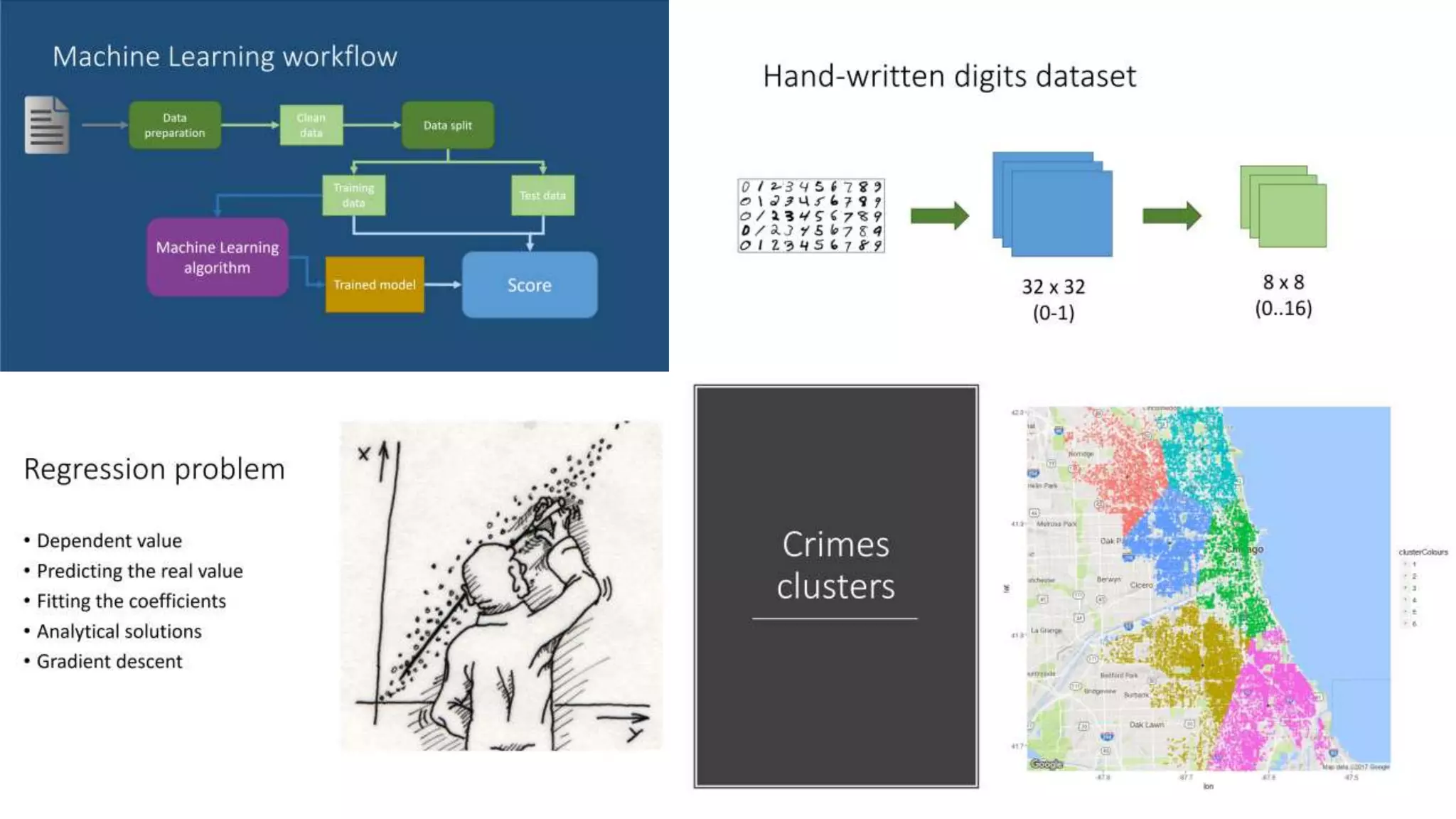

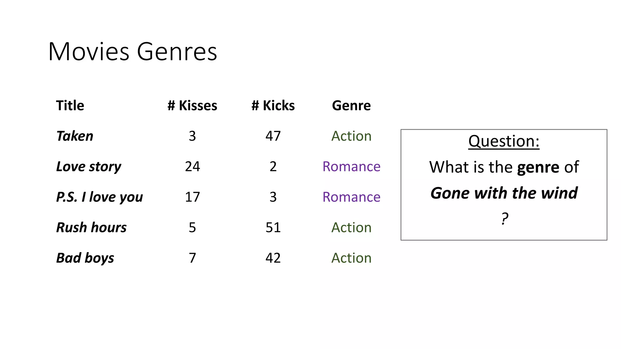
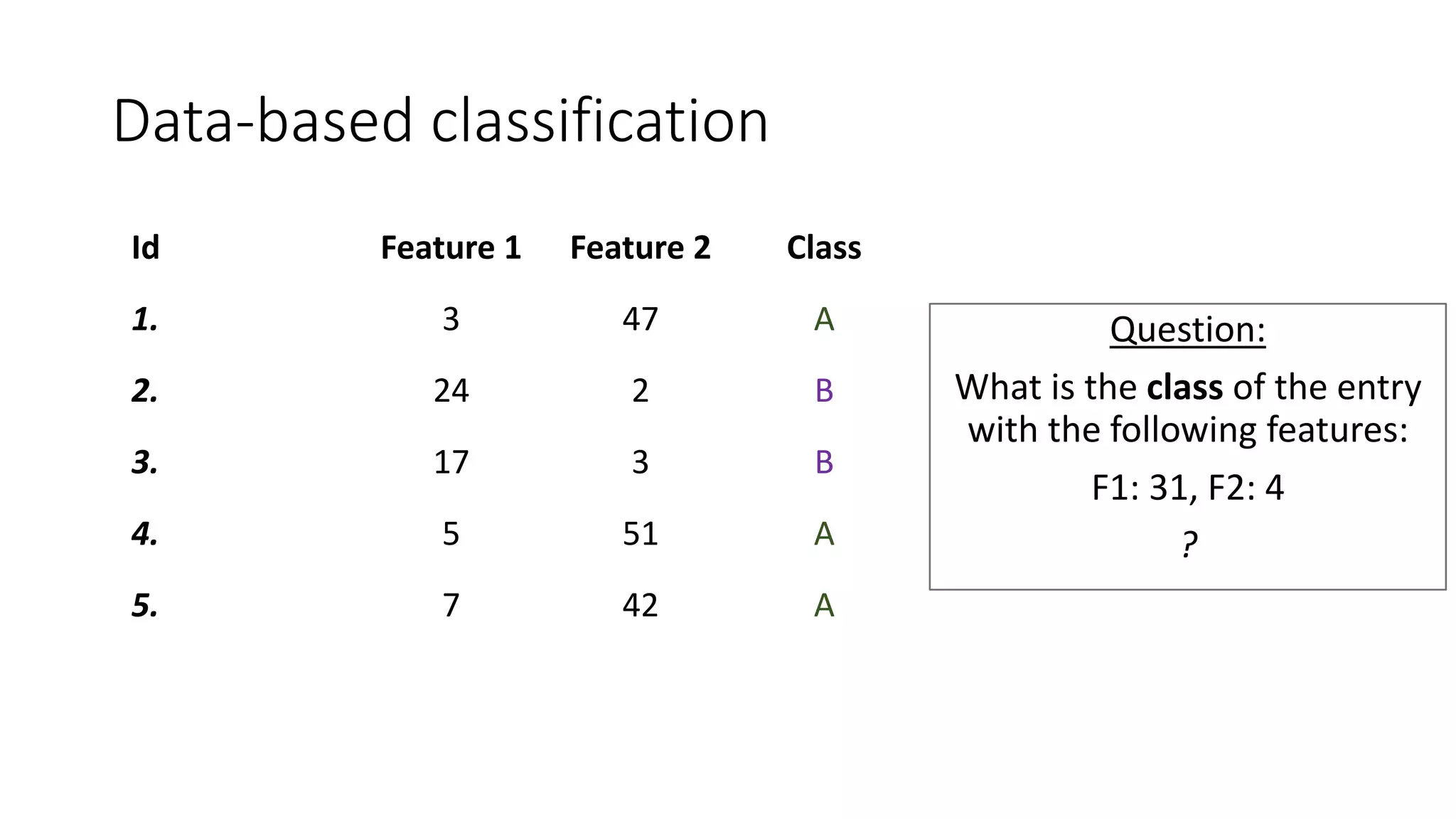
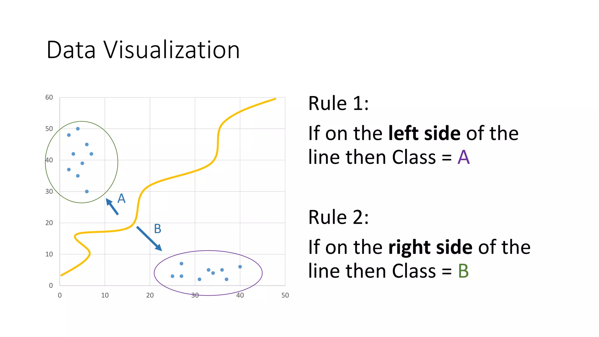
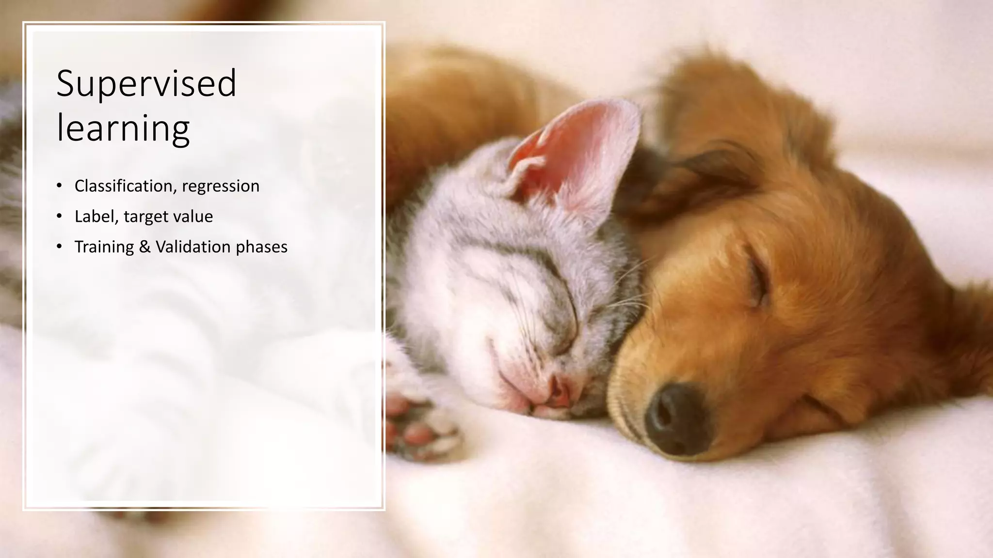
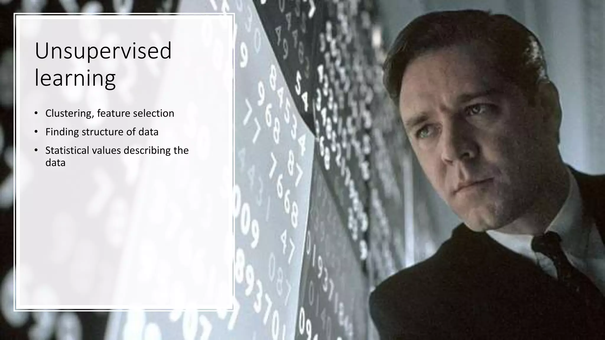
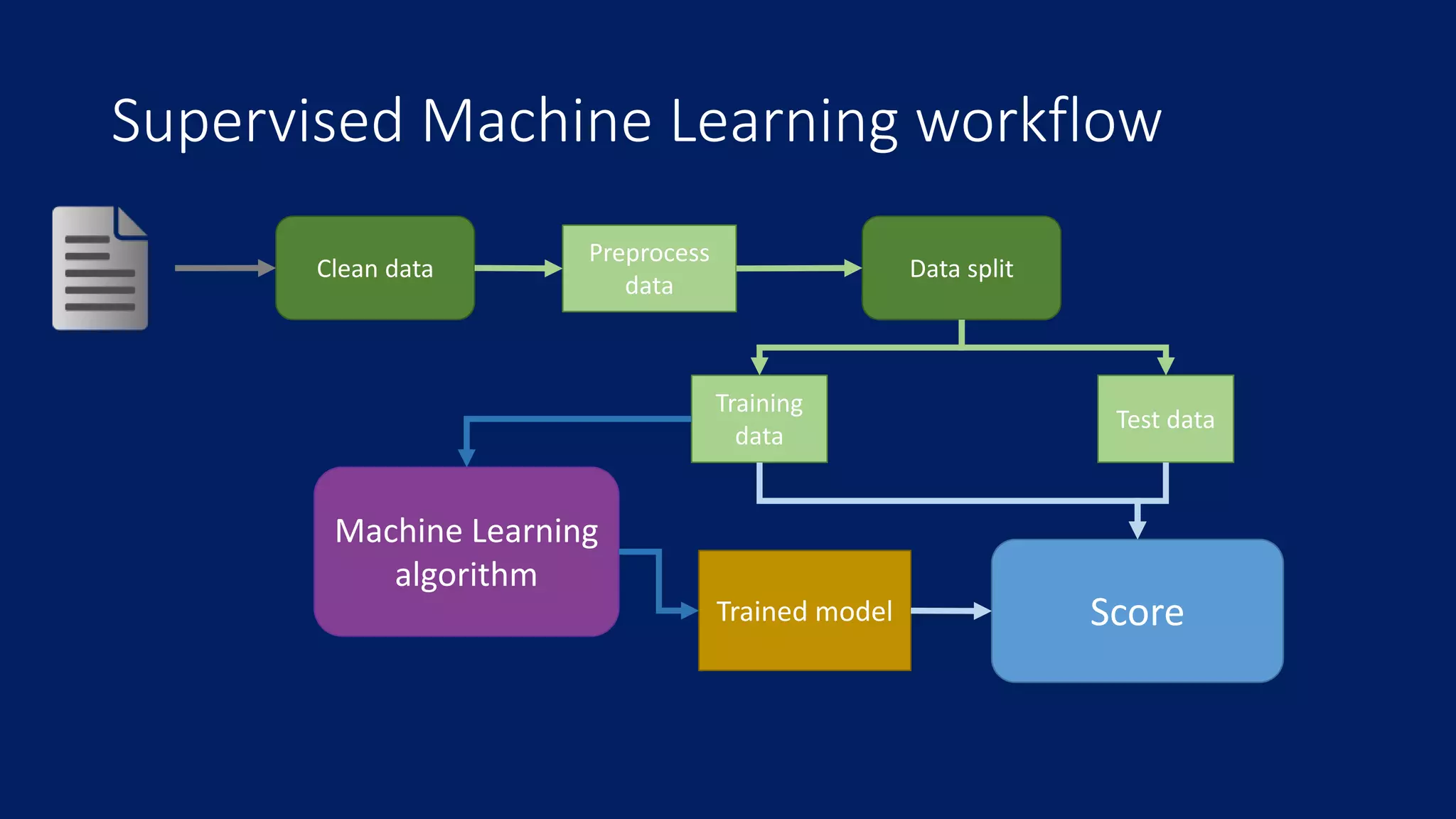
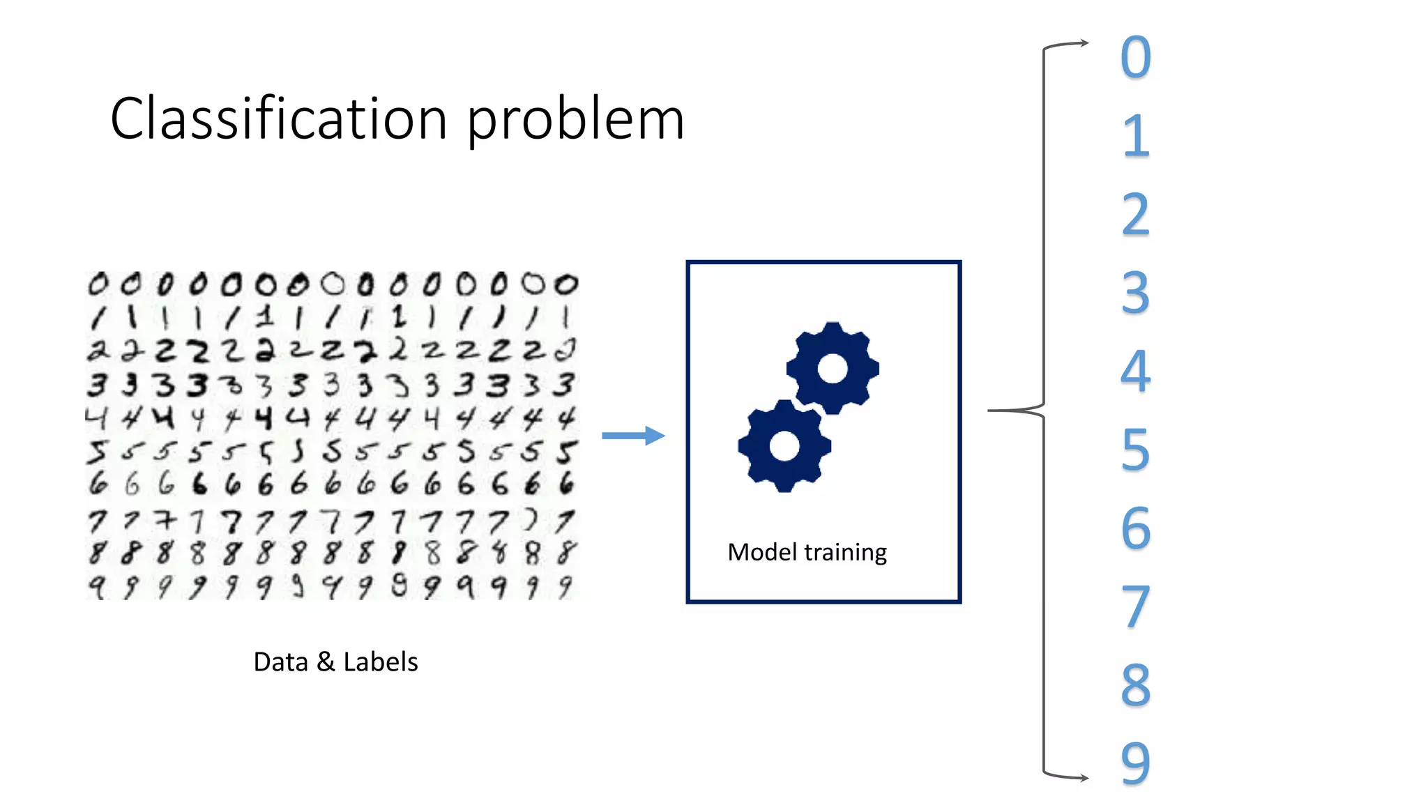
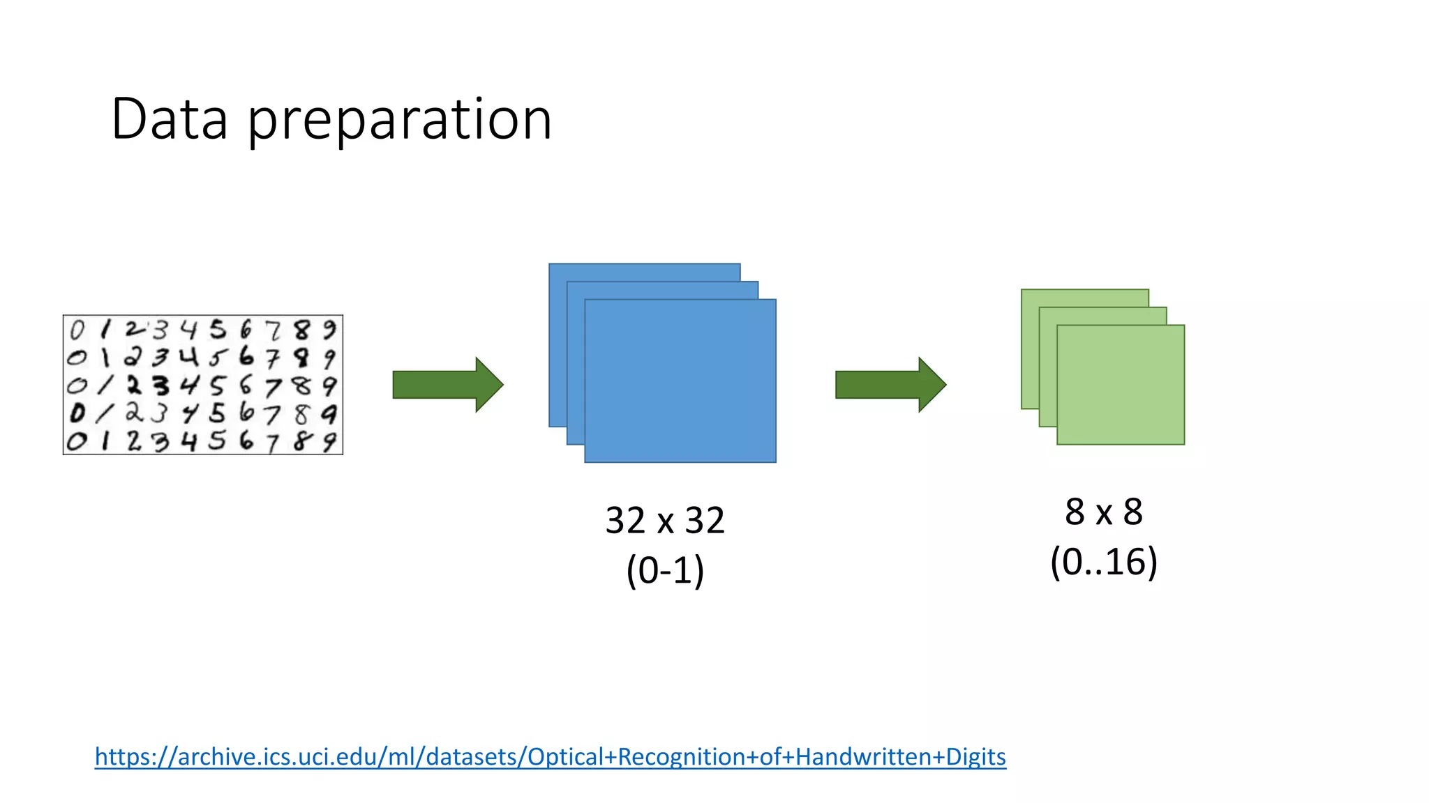
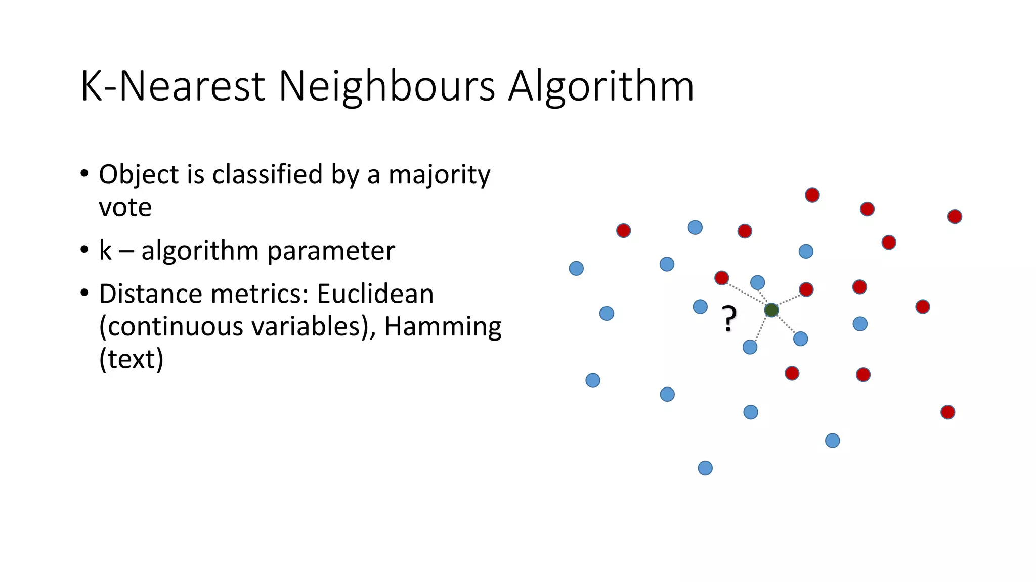
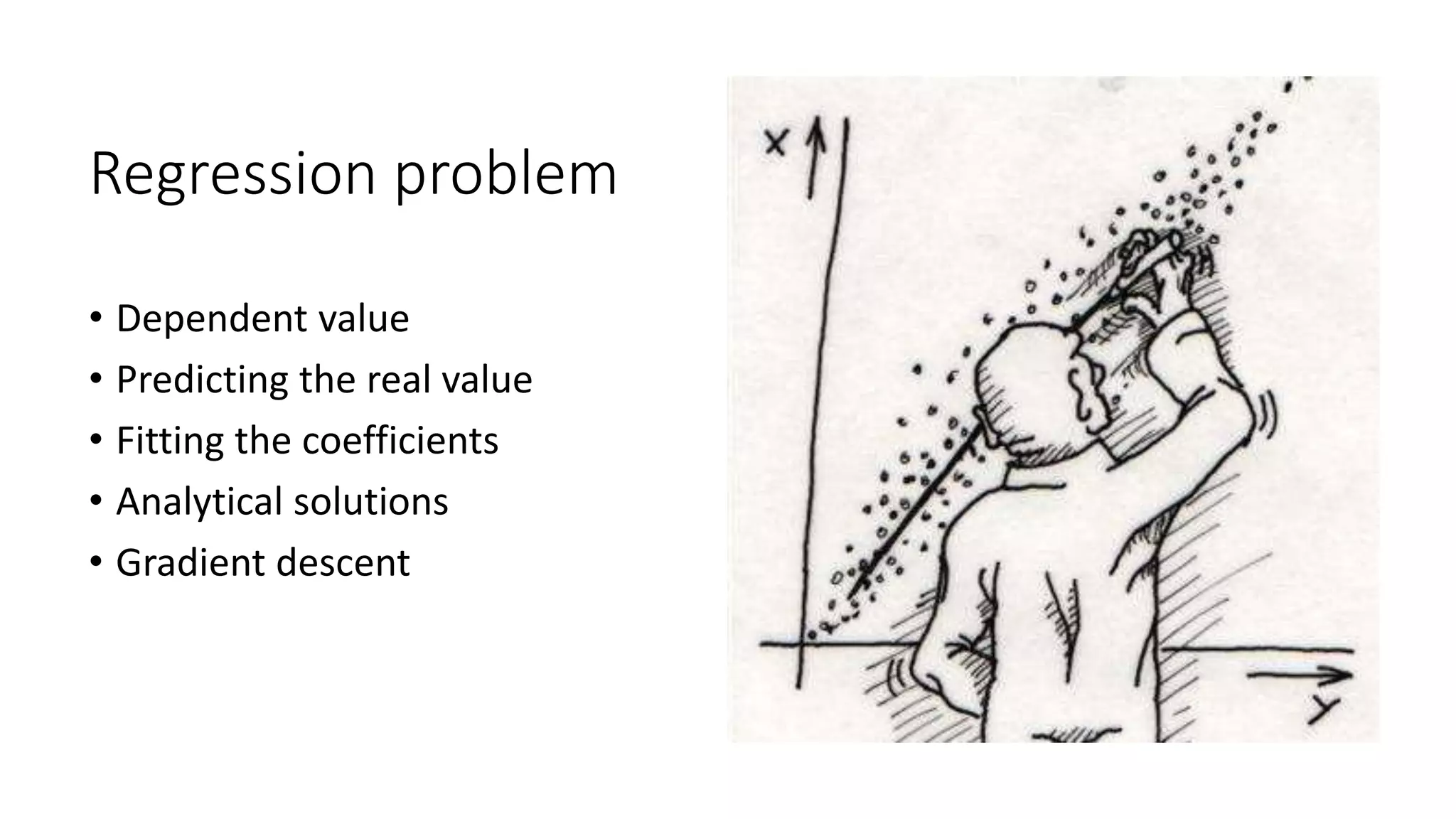
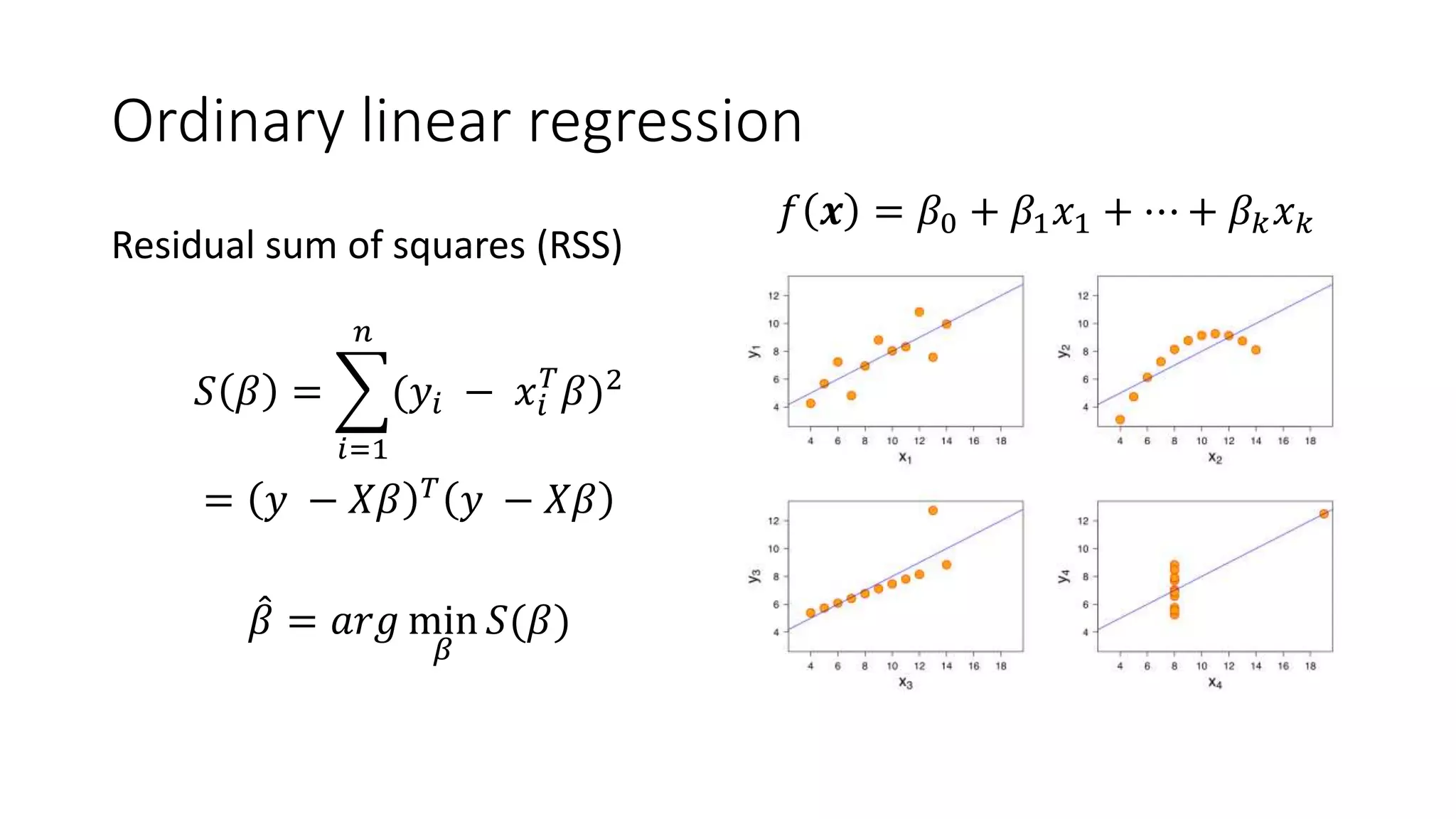
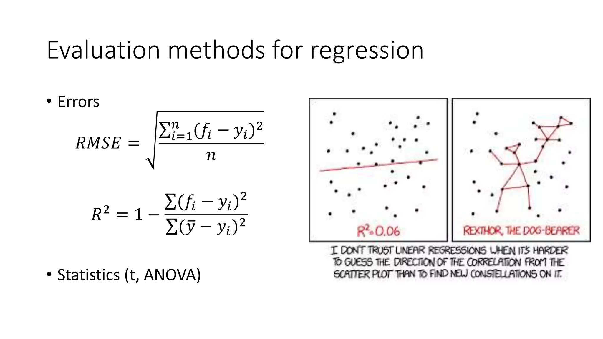
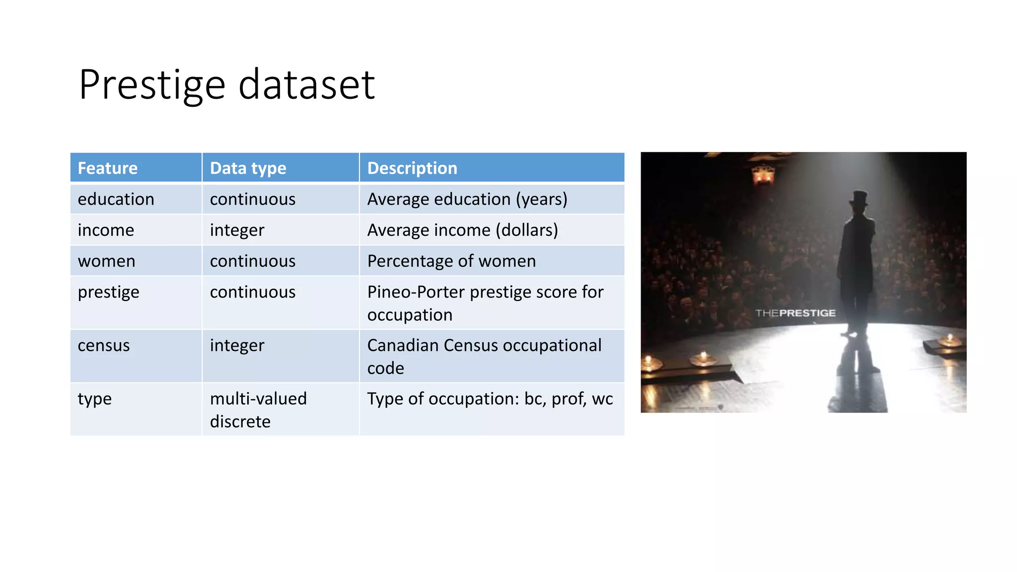
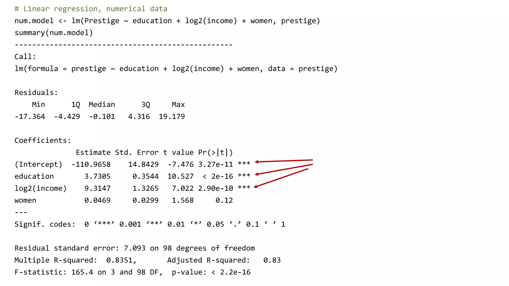
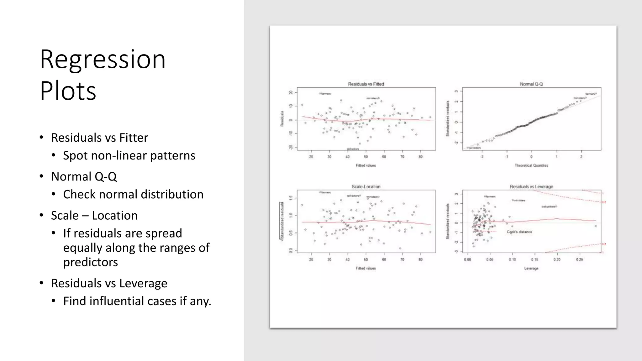
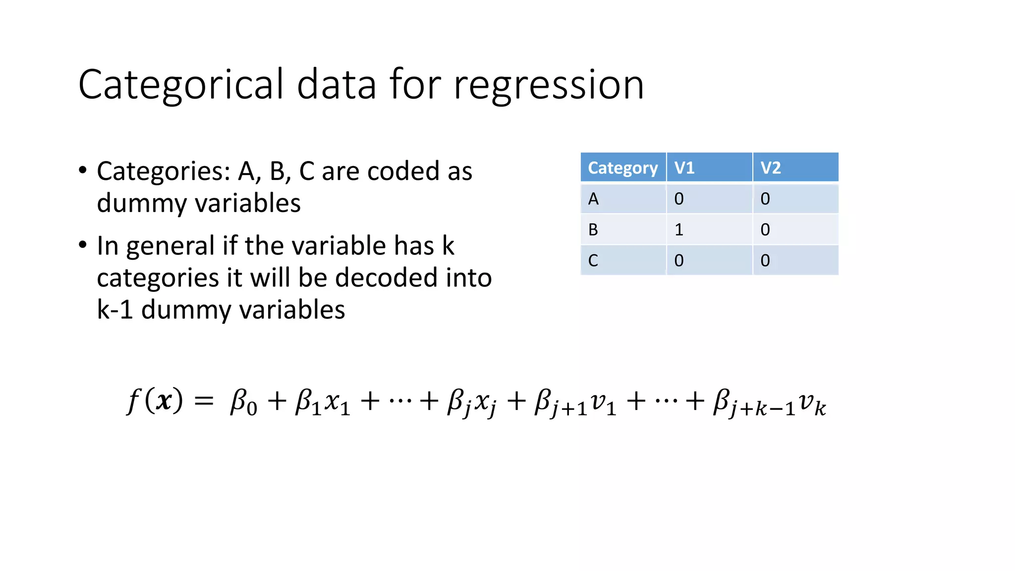
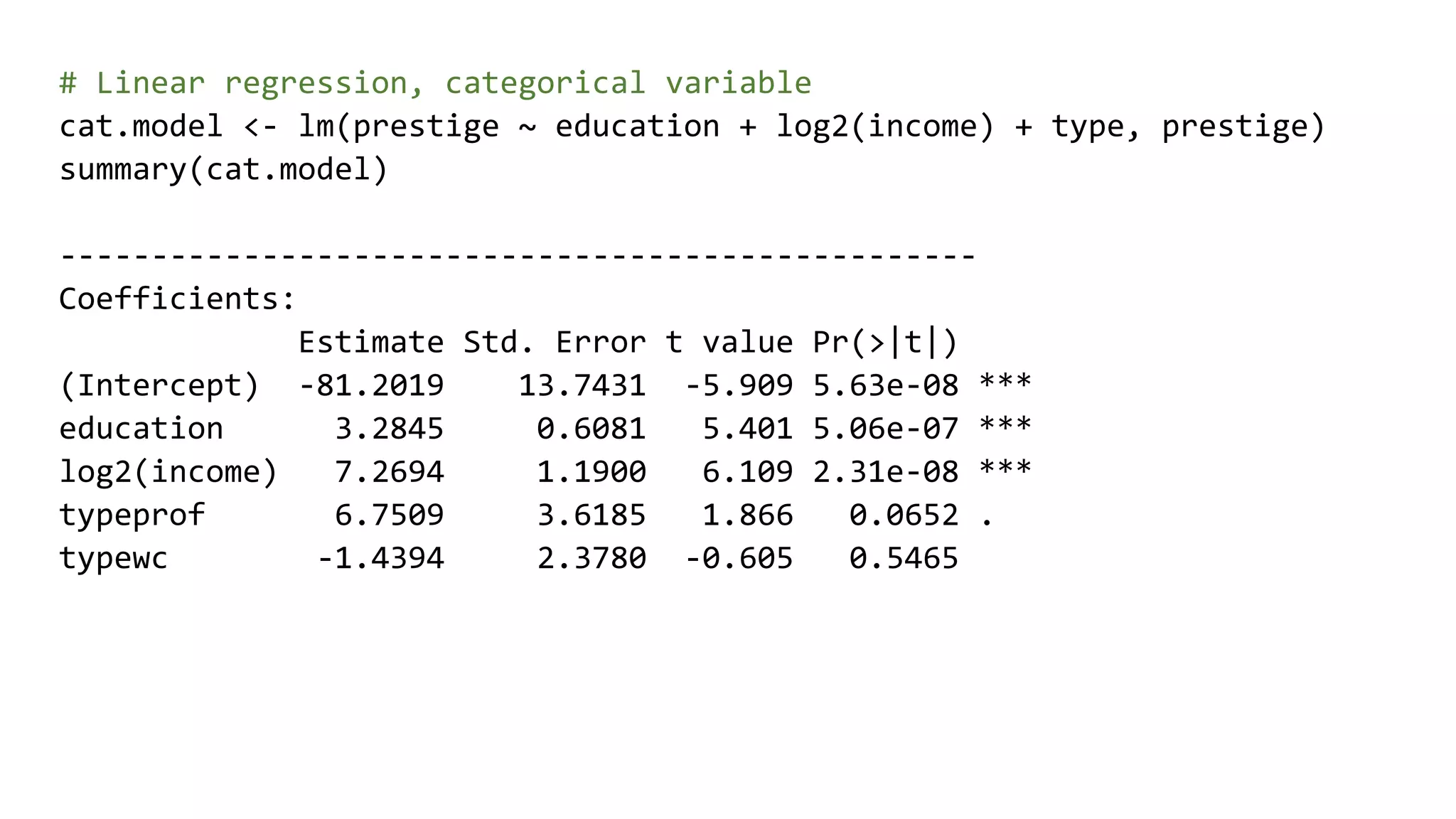
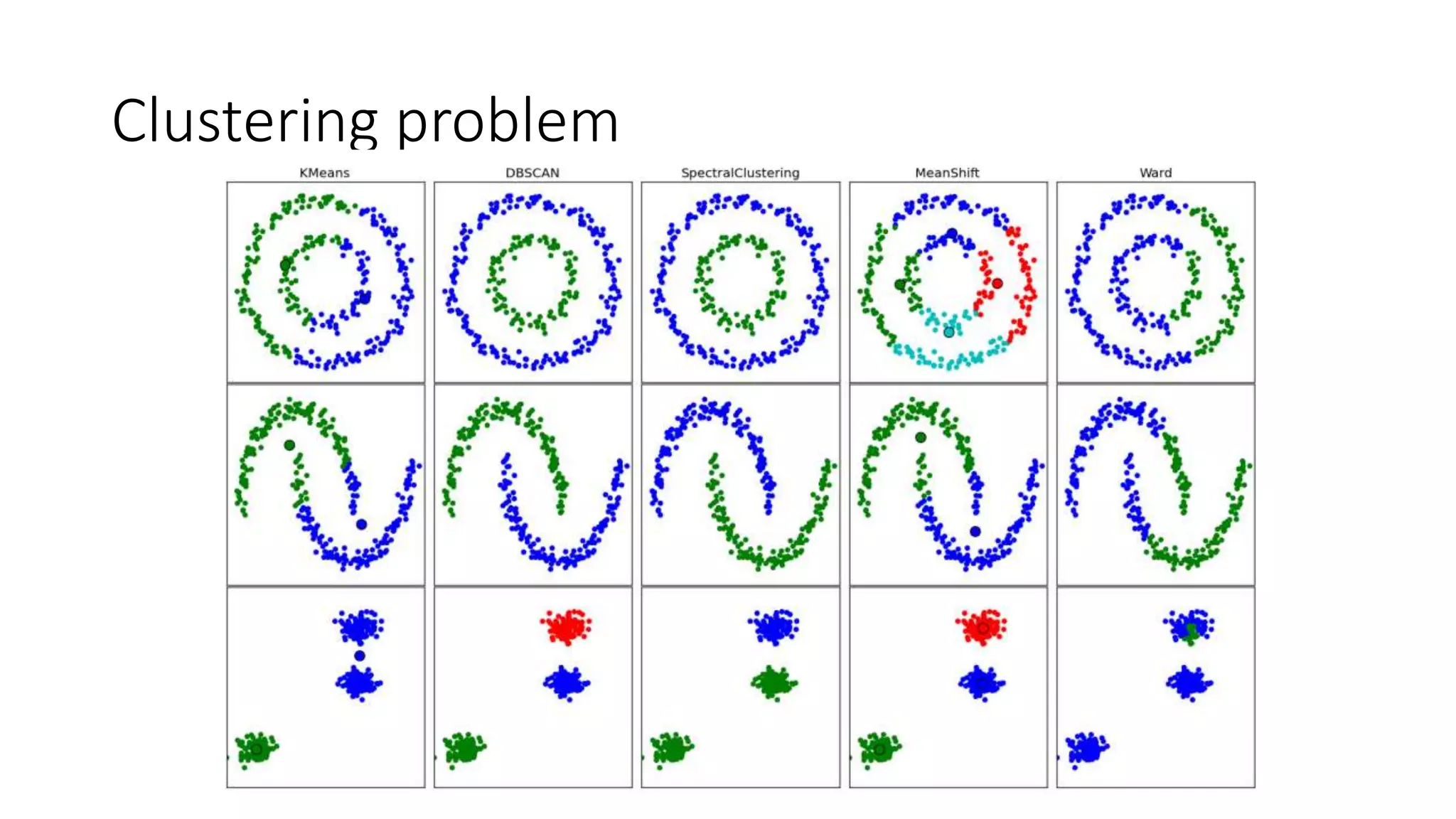
This document provides an overview of machine learning concepts and how to apply them using the R programming language. It introduces machine learning tasks like classification, regression, and clustering. For classification, it demonstrates linear regression on a movie genres dataset and k-nearest neighbors on a handwritten digits dataset. For regression, it fits linear models to a prestige dataset. For clustering, it applies k-means to group crimes in Chicago neighborhoods. Visualizations are shown throughout using R packages like ggplot and caret.