SQLBits Module 2 RStats Introduction to R and Statistics

The Data Analyst’s Toolkit Introduction to R Jen Stirrup | Data Relish Ltd| June, 2014 Jen.Stirrup@datarelish.com

Note • This presentation was part of a full day workshop on Power BI and R, held at SQLBits in 2014 • This is a sample, provided to help you see if my one day Business Intelligence Masterclass is the right course for you. • http://bit.ly/BusinessIntelligence2016Masterclass • In that course, you’ll be given updated notes along with a hands-on session, so why not join me? 2

Course Outline • Module 1: Setting up your data for R with Power Query • Module 2: Introducing R • Module 3: The Big Picture: Putting Power BI and R together • Module 4: Visualising your data with Power View and Excel 2013 • Module 5: Power Map • Module 6: Wrap up and Q and Q

What is R? 4 • R is a powerful environment for statistical computing • It is an overgrown calculator • … which lets you save results in variables x <- 3 y <- 5 z = 4 x + y + z

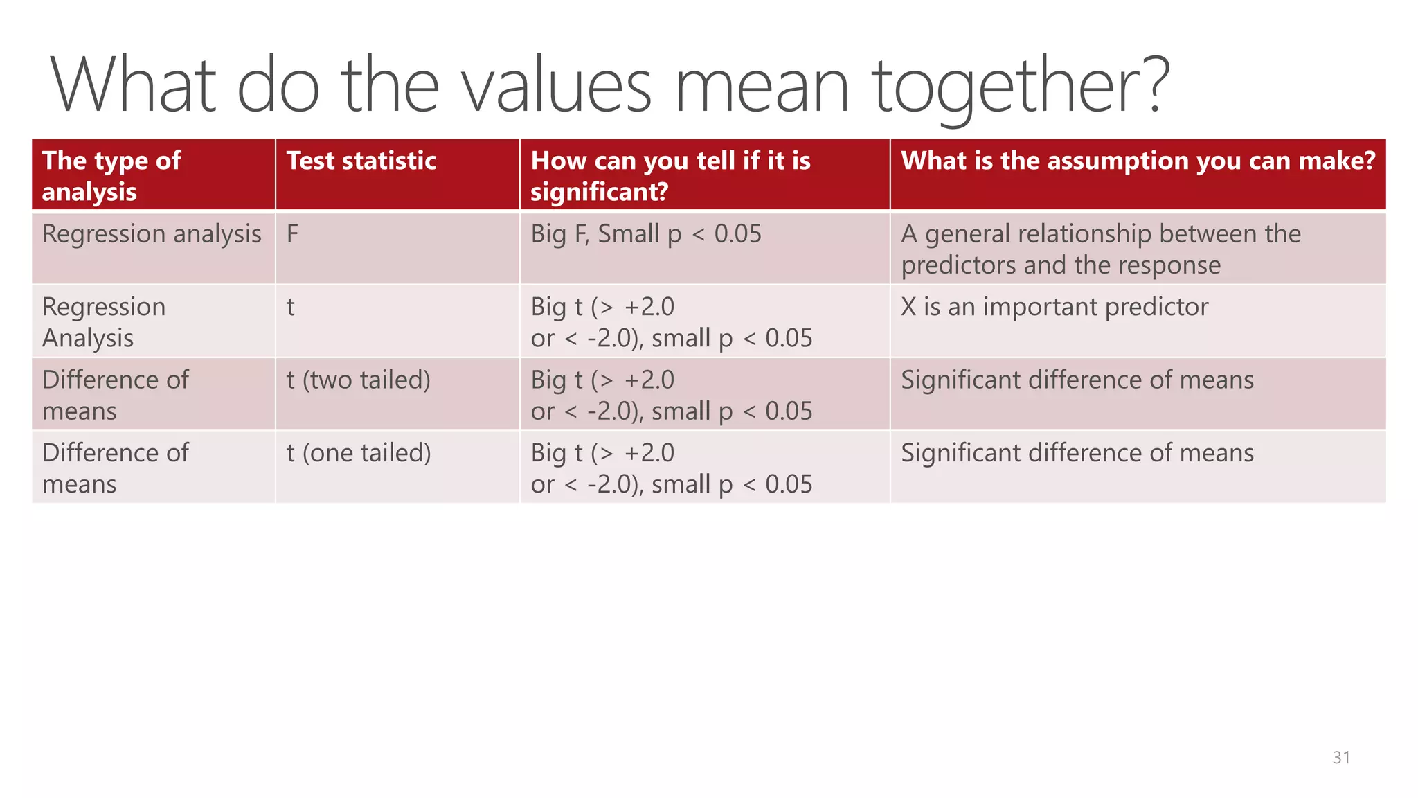
Vectors in R 5 • create a vector (list) of elements, use the "c" operator v = c("hello","world","welcome","to","the class.") v = seq(1,100) v[1] v[1:10] • Subscripting in R square brackets operators allow you to extract values: • insert logical expressions in the square brackets to retrieve subsets of data from a vector or list. For example:

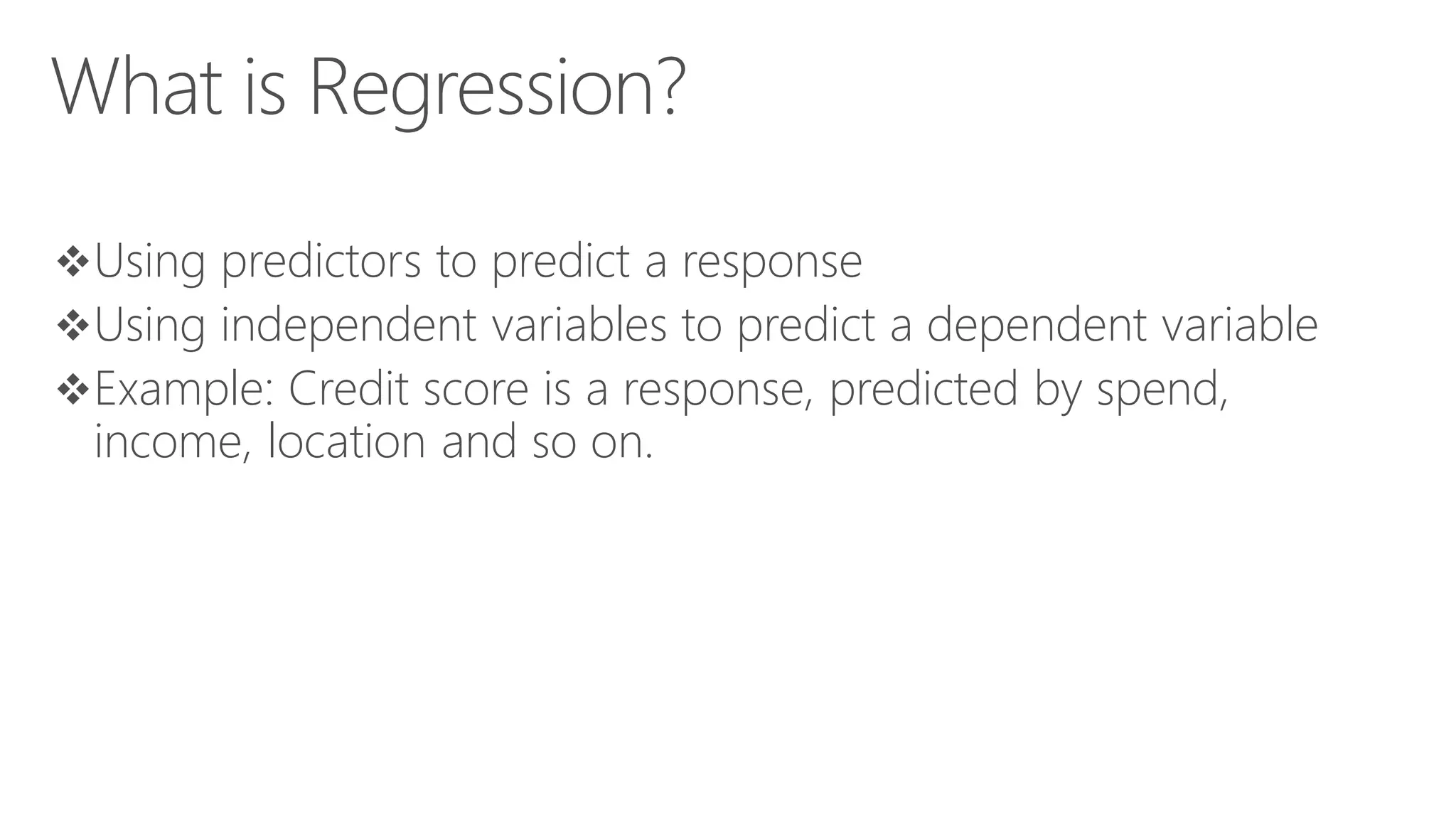
Vectors in R Microsoft Confidential 6 v = seq(1,100) logi = v>95 logi v[logi] v[v<6] v[105]=105 v[is.na(v)]

Save and Load RData Data is saved in R as .Rdata files Imported back again with load a <- 1:10 save(a, file = "E:/MyData.Rdata") rm(a) load("E:/MyData.Rdata") print(a)

Import From CSV Files • A simple way to load in data is to read in a CSV. • Read.csv() • MyDataFrame <- read.csv(“filepath.csv") • print(MyDataFrame)

Import From CSV Files • Go to Tools in RStudio, and select Import Dataset. • Select the file CountryCodes.csv and select the Import button. • In RStudio, you will now see the data in the data pane.

Import From CSV Files The console window will show the following: > #import dataset > CountryCodes <- read.csv("C:/Program Files/R/R- 3.1.0/Working Directory/CountryCodes.csv", header=F) > View(CountryCodes) Once the data is imported, we can check the data. dim(CountryCodes) head(CountryCodes) tail(CountryCodes)

Import / Export via ODBC • The Package RODBC provides R with a connection to ODBC databases • library(RODBC) • myodbcConnect <- odbcConnect(dsn="servername",uid="us erid",pwd="******")

Import / Export via ODBC • Query <- "SELECT * FROM lib.table WHERE ..." • # or read query from file myQuery <- readChar("E:/MyQueries/myQuery.sql", nchars=99999) myData <- sqlQuery(myodbcConnect, myQuery, errors=TRUE) odbcCloseAll()

Import/Export from Excel Files • RODBC also works for importing data from Excel files • library(RODBC) • filename <- "E:/Rtmp/dummmyData.xls" • myxlsFile <- odbcConnectExcel(filename, readOnly = FALSE) • sqlSave(myxlsFile, a, rownames = FALSE) • b <- sqlFetch(myxlsFile, "a") • odbcCloseAll()

Anscombe’s Quartet Property Value Mean of X 9 Variance of X 11 Mean of Y 7.50 Variance of Y 4.1 Correlation 0.816 Linear Regression Y = 3.00 + 0.5 14

What does Anscombe’s Quartet look like? 15

Correlation r = 0.96 18 2000 2001 2002 2003 2004 2005 2006 2007 2008 2009 Number of people who died by becoming tangled in their bedsheets Deaths (US) (CDC) 327 456 509 497 596 573 661 741 809 717 Total revenue generated by skiing facilities (US) Dollars in millions (US Census) 1,551 1,635 1,801 1,827 1,956 1,989 2,178 2,257 2,476 2,438

R and Power BI together • Pivot Tables are not always enough • Scaling Data (ScaleR) • R is very good at static data visualisation • Upworthy 19

Why R? • most widely used data analysis software - used by 2M + data scientist, statisticians and analysts • Most powerful statistical programming language • flexible, extensible and comprehensive for productivity • Create beautiful and unique data visualisations - as seen in New York Times, Twitter and Flowing Data • Thriving open-source community - leading edge of analytics research • Fills the talent gap - new graduates prefer R. 20

Growth in Demand • Rexer Data Mining survey, 2007 - 2013 • R is the highest paid IT skill Dice.com, Jan 2014 • R most used-data science language after SQL - O'Reilly, Jan 2014 • R is used by 70% of data miners. Rexer, Sept 2013 21

Growth in Demand • R is #15 of all programming languages. • RedMonk, Jan 2014 • R growing faster than any other data science language. • KDNuggets. • R is in-memory and limited in the size of data that you can process. 22

What are we testing? • We have one or two samples and a hypothesis, which may be true or false. • The NULL hypothesis – nothing happened. • The Alternative hypothesis – something did happen. 23

Strategy • We set out to prove that something did happen. • We look at the distribution of the data. • We choose a test statistic • We look at the p value 24

How small is too small? • How do we know when the p-value is small? • P => 0.05 – Null hypothesis is true • P < 0.05 – alternative hypothesis is true • it depends • For high-risk, then perhaps we want 0.01 or even 0.001. 25

Confidence Intervals • Basically, how confident are you that you can extrapolate from your little data set to the larger population? • We can look at the mean • To do this, we run a t.test • t.test(vector) 26

Confidence Intervals • Basically, how confident are you that you can extrapolate from your little data set to the larger population? • We can look at the median • To do this, we run a Wilcox test. • t.test(vector) 27

Calculate the relative frequency • How much is above, or below the mean? • Mean(after > before) • Mean(abs(x-mean)) < 2 *sd(s) • This gives you the fraction of data that is greater than two standard deviations from the mean. 28

Testing Categorical Variables for Independence • Chi squares – are two variables independent? Are they connected in some way? • Summarise the data first: Summary(table(initial, outcome)) • chisq.test 29

How Statistics answers your question • Is our model significant or insignificant? – The F Statistic • What is the quality of the model? – R2 statistic • How well do the data points fit the model? – R2 statistic

What do the values mean together? The type of analysis Test statistic How can you tell if it is significant? What is the assumption you can make? Regression analysis F Big F, Small p < 0.05 A general relationship between the predictors and the response Regression Analysis t Big t (> +2.0 or < -2.0), small p < 0.05 X is an important predictor Difference of means t (two tailed) Big t (> +2.0 or < -2.0), small p < 0.05 Significant difference of means Difference of means t (one tailed) Big t (> +2.0 or < -2.0), small p < 0.05 Significant difference of means 31

What is Regression? Using predictors to predict a response Using independent variables to predict a dependent variable Example: Credit score is a response, predicted by spend, income, location and so on.

Linear Regression using World Bank data We can look at predicting using World Bank data Year <- GDP <- (wdiData, ) Plot(wdiData, Cor(year, wdiData) Fit <- lm(cpi ~ year+quarter) Fit

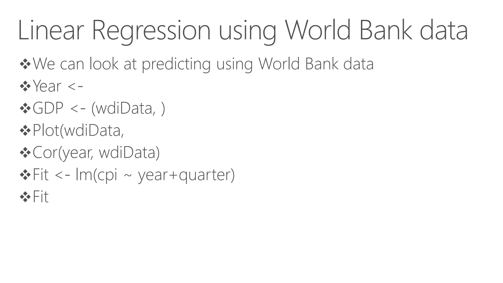
Examples of Data Mining in R  cpi2011 <- fit$coefficients[[1]] + fit$coefficients[[2]]*2011 + fit$coefficients[[3]]*(1:4) attributes(fit) fit$coefficients Residuals(fit) – difference between observed and fitted values Summary(fit) Plot(fit)

What is Data Mining Machine Learning Statistics Software Engineering and Programming with Data Intuition Fun!

The Why of Data Mining to discover new knowledge to improve business outcomes to deliver better customised services

Examples of Data Mining in R Logistic Regression (glm) Decision Trees (rpart, wsrpart) Random Forests (randomForest, wsrf) Boosted Stumps (ada) Neural Networks (nnet) Support Vector Machines (kernlab)

Examples of Data Mining in R • Packages: – fpc – cluster – pvclust – mclust • Partitioning-based clustering: kmeans, pam, pamk, clara • Hierarchical clustering: hclust, pvclust, agnes, Diana • Model-based clustering: mclust • Density-based clustering: dbscan • Plotting cluster solutions: plotcluster, plot.hclust • Validating cluster solutions: cluster.stats

How can we make it easier? • AzureML

The Data Mining Process • Load data • Choose your variables • Sample the data into test and training sets (usually 70/30 split) • Explore the distributions of the data • Test some distributions • Transform the data if required • Build clusters with the data • Build a model • Evaluate the model • Log the data process for auditing externally

Loading the Data • Dsname is the name of our dataset • Get(dsname) • Dim(ds) • Names(ds)

Explore the data • Head(dataset) • Tail(dataset)

Explore the data’s structure • Str(dataset) • Summary(dataset)

Pick out the Variables • Id <- c(“Date”, “Location) target <- “RainTomorrow” risk <- “RISK_MM” • (ignore <-union(id, risk)) • (vars <- setdiff(names(ds), ignore))

Remove Missing Data • dim(ds) ## [1] 366 24 sum(is.na(ds[vars])) • ## [1] 47 ds <- ds[-attr(na.omit(ds[vars]), "na.action"),] • dim(ds) ## [1] 328 24 sum(is.na(ds[vars])) • ## [1] 0

Clean Data Target as Categorical Data • summary(ds[target]) • ## RainTomorrow ## Min. :0.000 ## 1st Qu.:0.000 • ## Median :0.000 ## Mean :0.183 ## 3rd Qu.:0.000 ## Max. :1.000 • .... • ds[target] <- as.factor(ds[[target]]) levels(ds[target]) <- c("No", "Yes") • summary(ds[target])

Model Preparation • (form <- formula(paste(target, "~ ."))) ## RainTomorrow ~ . • (nobs <- nrow(ds)) ## [1] 328 • train <- sample(nobs, 0.70*nobs) length(train) ## [1] 229 • test <- setdiff(1:nobs, train) length(test) • ## [1] 99

Random Forest • library(randomForest) model <- randomForest(form, ds[train, vars], na.action=na.omit) model • ## • ## Call: • ## randomForest(formula=form, data=ds[train, vars], ... • ## Type of random forest: classification • ## Number of trees: 500 • ## No. of variables tried at each split: 4 ....

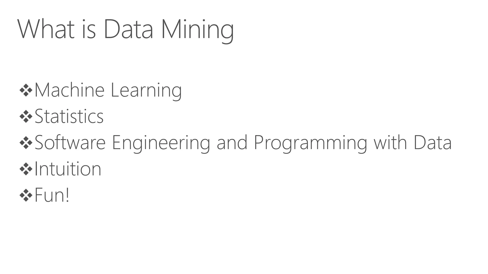
Evaluate the Model – Risk Chart • pr <- predict(model, ds[test,], type="prob")[,2] riskchart(pr, ds[test, target], ds[test, risk], • title="Random Forest - Risk Chart", risk=risk, recall=target, thresholds=c(0.35, 0.15))

Linear Regression • X: predictor variable • Y: response variable • Lm( y ~ x, data= dataframe)

Multiple Linear Regression • Lm is used again • Lm( y ~ x + u + v, data frame) • It is better to keep the data in one data frame because it is easier to manage.

Getting Regression Statistics • Save the model to a variable: • M <- lm(y ~ x + u + v) • Then use regression statistics to get the values that you need from m.

Getting Regression Statistics • Anova(m) • Coefficients(m) / coef(m) • Confint(m) • Effects(m) • Fitted(m) • Residuals(m)

Getting regression statistics • The most important one is summary(m). It shows: • Estimated coefficients • Critical statistics such as R2 and the F statistic • The output is hard to read so we will write it out to Excel.

Understanding the Regression Summary • The model summary gives you the information for the most important regression statistics, such as the residuals, coefficients and the significance codes. • The most important one is the F statistic. • You can check the residuals whether they are a normal distribution or not. How can you tell this?

Understanding the Regression Summary • The direction of the median is important e.g. a negative direction will tell you if there is a skew to the left. • The quartiles will also help. Ideally Q1 and Q3 should have the same magnitude. If not, a skew has developed. This could be inconsistent with the median result. • It helps us to identify outliers.

Coefficients and R • The Estimate column contains estimated regression coefficients, calculated using the least squares method. This is the most common method. • How likely is it that the coefficients are zero? This only shows estimates. This is the purpose of the column t and p ( > ¦ t¦)

Coefficients and R • The p value is a probability that this finding is significant. The lower, the better. We can look at the column signif. codes to help us to identify the most appropriate level of p value.

Coefficients and R • R2 is the coefficient of determination. How successful is the model? We look at this value. Bigger is better. It is the variance of y that is explained by the regression model. The remaining variance is not explained by the model. The adjusted value takes into account the number of variables in the model.

First Impressions • Plotting the model can help you to investigate it further. • Library(car) • Outlier.test(m) • M <- lm(y ~ m) • Plot(m, which=1)

First Impressions? • How do you go about it? • Check the plot first; how does it look?

The F Statistic • Is the model significant or insignificant? This is the purpose of the F statistic. • Check the F statistic first because if it is not significant, then the model doesn’t matter.

Significance Stars The stars are shorthand for significance levels, with the number of asterisks displayed according to the p-value computed. *** for high significance and * for low significance. In this case, *** indicates that it's unlikely that no relationship exists b/w heights of parents and heights of their children.

Plot the Predicted Values • data2011 <- data.frame(year=2011, quarter=1:4) • > cpi2011 <- predict(fit, newdata=data2011) > style <- c(rep(1,12), rep(2,4)) • > plot(c(cpi, cpi2011), xaxt="n", ylab="CPI", xlab="", pch=style, col=style) • > axis(1, at=1:16, las=3, + labels=c(paste(year,quarter,sep="Q"), "2011Q1", "2011Q2", "2011Q3", "2011Q4"))

How to get Help Microsoft Confidential 65 example(rnorm) Rseek.org

Resources • Introductory Statistics with R by Peter Dalgaard. Good for beginners. • The Art of R Programming • http://www.r-project.org • CRAN sites – Comprehensive R Archive Network

SQLBits Module 2 RStats Introduction to R and Statistics

More Related Content

What's hot

Viewers also liked

Similar to SQLBits Module 2 RStats Introduction to R and Statistics

More from Jen Stirrup

Recently uploaded

SQLBits Module 2 RStats Introduction to R and Statistics