Download as PDF, PPTX


![15 Group Functions Syntax SELECT [column,] group_function(column). . . FROM table [WHERE condition] [GROUP BY group_by_expression] [ORDER BY column]; SELECT AVG(salary), STDDEV(salary), COUNT(commission_pct),MAX(hire_date) FROM hr.employees WHERE job_id LIKE 'SA%';](https://image.slidesharecdn.com/15102-oracledatabaseadvancedqueryingfinal-161128213310/75/Oracle-Database-Advanced-Querying-2016-15-2048.jpg)
![16 SELECT department_id, job_id, SUM(salary), COUNT(employee_id) FROM hr.employees GROUP BY department_id, job_id Order by department_id; The GROUP BY Clause SELECT [column,] group_function(column) FROM table [WHERE condition] [GROUP BY group_by_expression] [ORDER BY column];](https://image.slidesharecdn.com/15102-oracledatabaseadvancedqueryingfinal-161128213310/75/Oracle-Database-Advanced-Querying-2016-16-2048.jpg)
![17 The HAVING Clause • Use the HAVING clause to specify which groups are to be displayed • You further restrict the groups on the basis of a limiting condition SELECT [column,] group_function(column)... FROM table [WHERE condition] [GROUP BY group_by_expression] [HAVING having_expression] [ORDER BY column];](https://image.slidesharecdn.com/15102-oracledatabaseadvancedqueryingfinal-161128213310/75/Oracle-Database-Advanced-Querying-2016-17-2048.jpg)
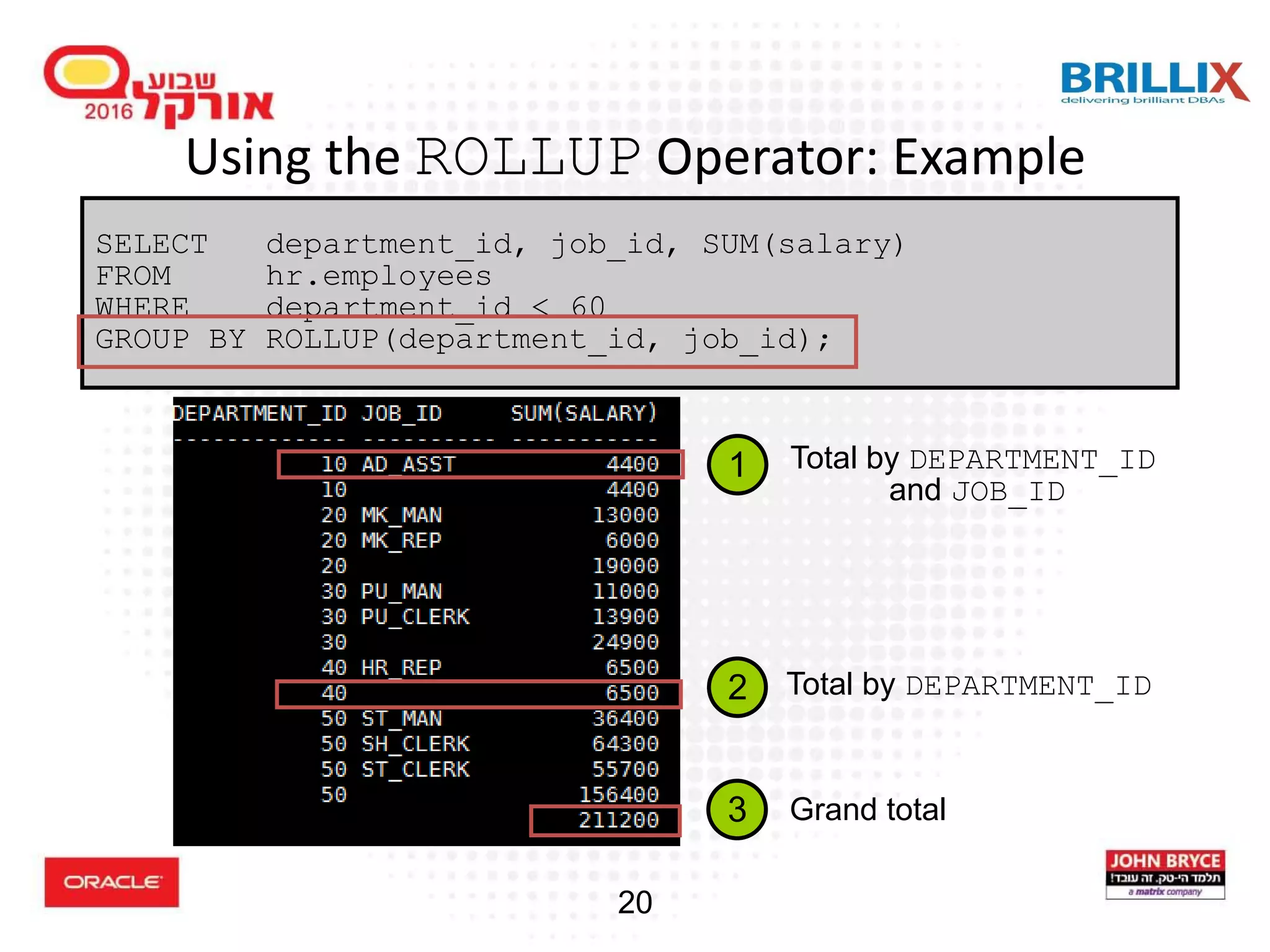
![19 Using the ROLLUP Operator • ROLLUP is an extension of the GROUP BY clause • Use the ROLLUP operation to produce cumulative aggregates, such as subtotals SELECT [column,] group_function(column). . . FROM table [WHERE condition] [GROUP BY [ROLLUP] group_by_expression] [HAVING having_expression]; [ORDER BY column];](https://image.slidesharecdn.com/15102-oracledatabaseadvancedqueryingfinal-161128213310/75/Oracle-Database-Advanced-Querying-2016-19-2048.jpg)
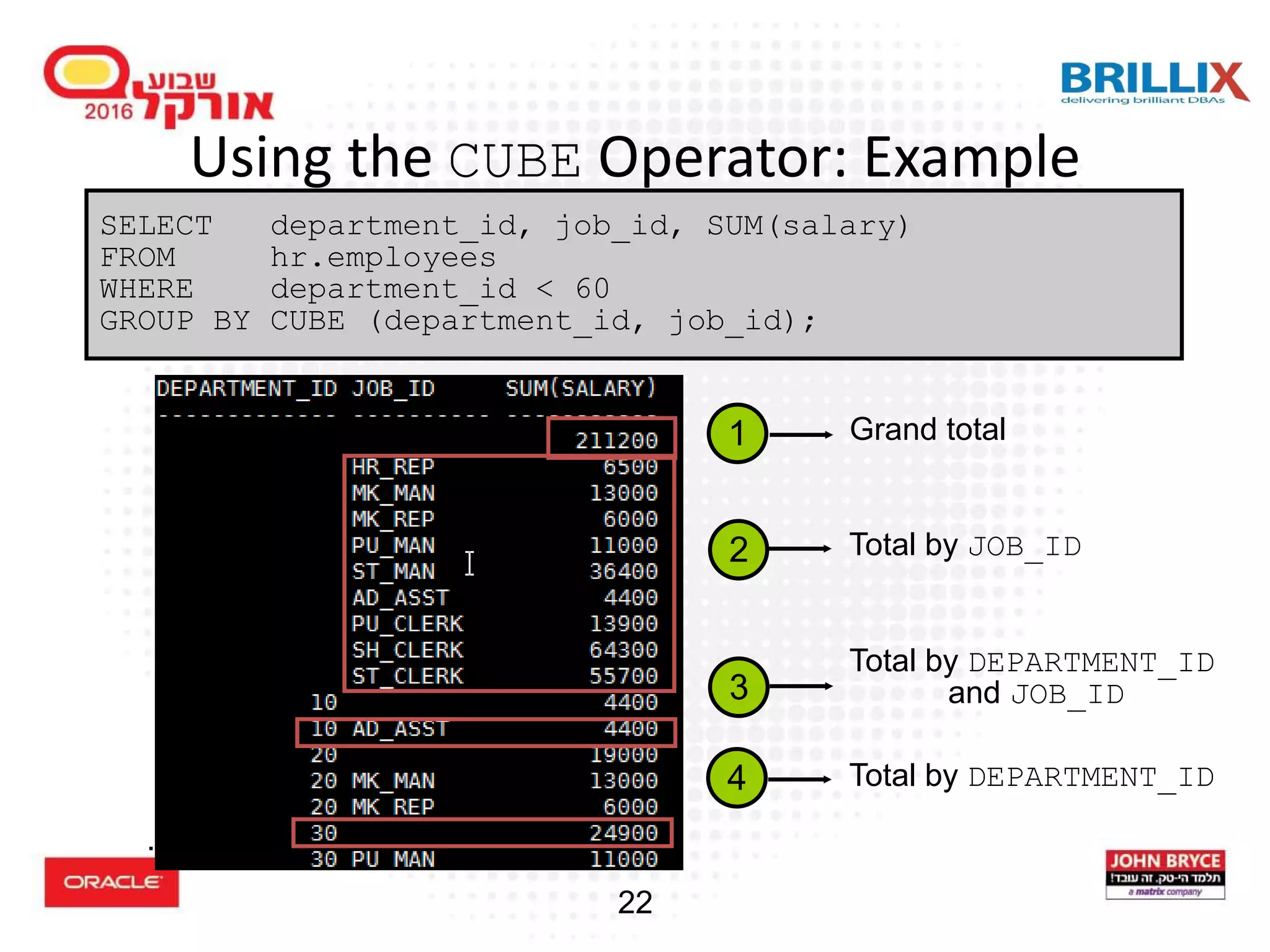
![21 Using the CUBE Operator • CUBE is an extension of the GROUP BY clause • You can use the CUBE operator to produce cross- tabulation values with a single SELECT statement SELECT [column,] group_function(column)... FROM table [WHERE condition] [GROUP BY [CUBE] group_by_expression] [HAVING having_expression] [ORDER BY column];](https://image.slidesharecdn.com/15102-oracledatabaseadvancedqueryingfinal-161128213310/75/Oracle-Database-Advanced-Querying-2016-21-2048.jpg)
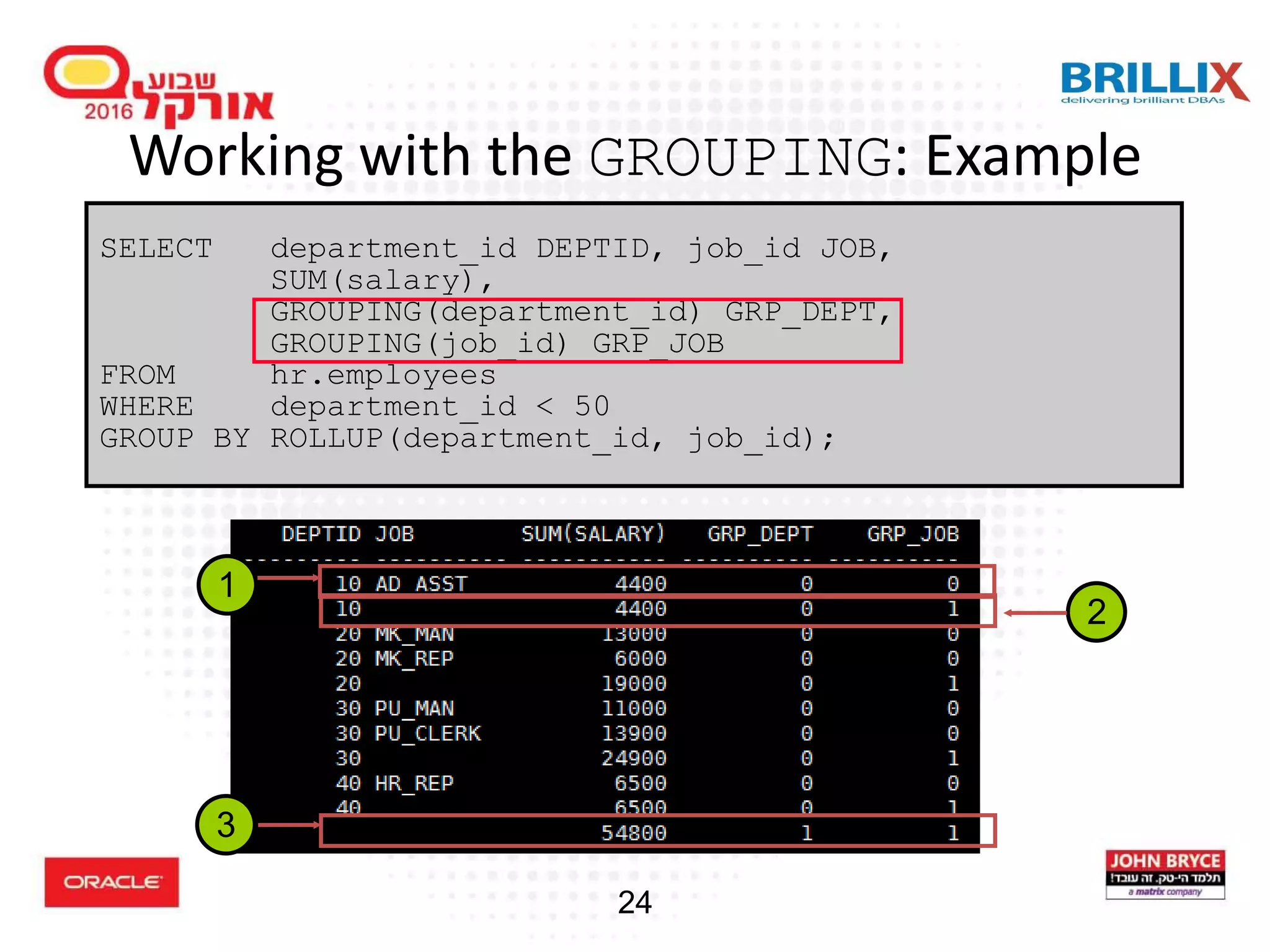
![23 SELECT [column,] group_function(column) .. , GROUPING(expr) FROM table [WHERE condition] [GROUP BY [ROLLUP][CUBE] group_by_expression] [HAVING having_expression] [ORDER BY column]; Working with the GROUPING Function • The GROUPING function: – Is used with the CUBE or ROLLUP operator – Is used to find the groups forming the subtotal in a row – Is used to differentiate stored NULL values from NULL values created by ROLLUP or CUBE – Returns 0 or 1](https://image.slidesharecdn.com/15102-oracledatabaseadvancedqueryingfinal-161128213310/75/Oracle-Database-Advanced-Querying-2016-23-2048.jpg)

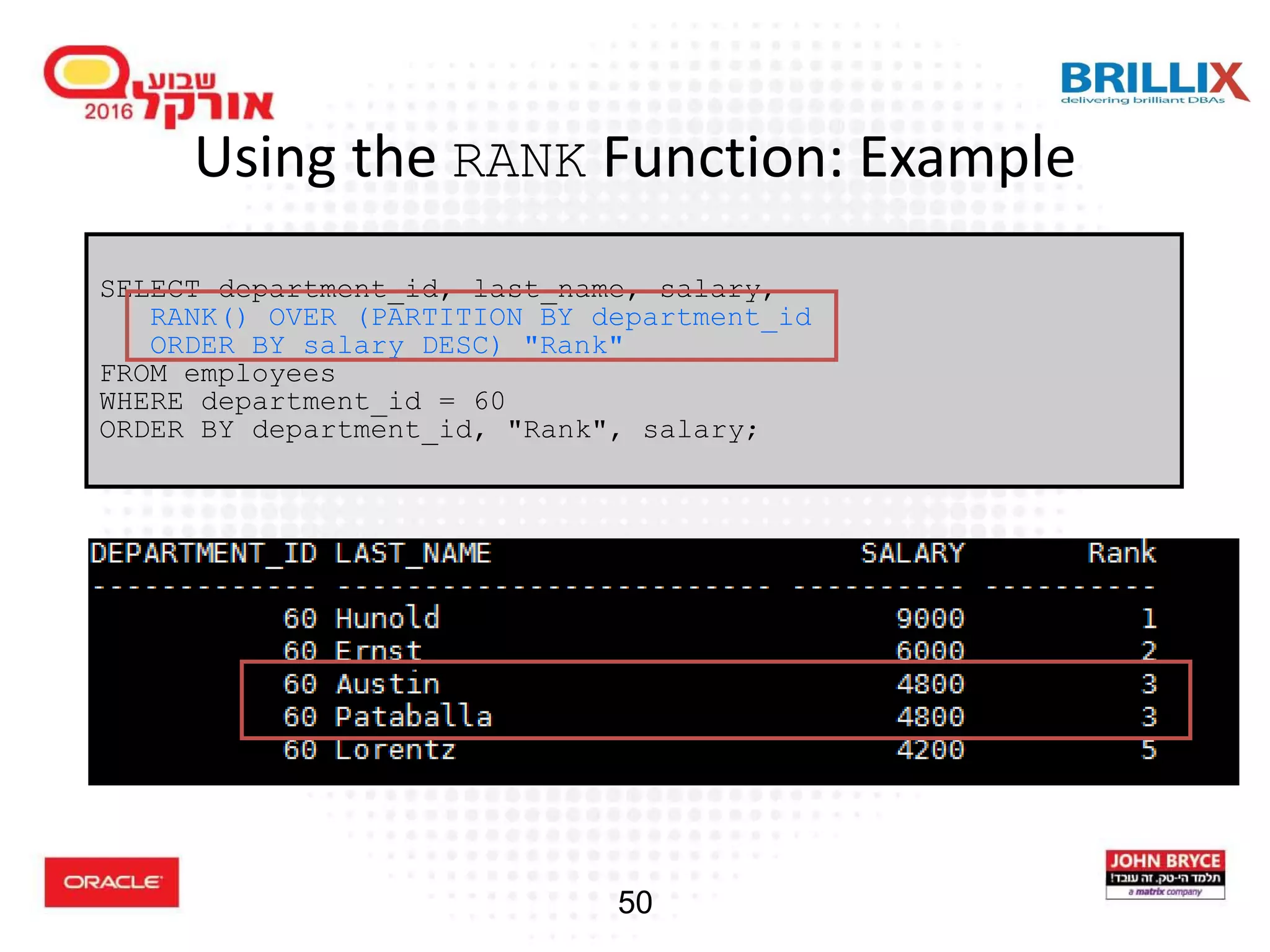
![49 Working with the RANK Function • The RANK function calculates the rank of a value in a group of values, which is useful for top-N and bottom-N reporting. • For example, you can use the RANK function to find the top ten products sold in Boston last year. • When using the RANK function, ascending is the default sort order, which you can change to descending. • Rows with equal values for the ranking criteria receive the same rank. • Oracle Database then adds the number of tied rows to the tied rank to calculate the next rank. RANK ( ) OVER ( [query_partition_clause] order_by_clause )](https://image.slidesharecdn.com/15102-oracledatabaseadvancedqueryingfinal-161128213310/75/Oracle-Database-Advanced-Querying-2016-44-2048.jpg)
![53 RANK and DENSE_RANK Functions: Example SELECT department_id, last_name, salary, RANK() OVER (PARTITION BY department_id ORDER BY salary DESC) "Rank", DENSE_RANK() over (partition by department_id ORDER BY salary DESC) "Drank" FROM employees WHERE department_id = 60 ORDER BY department_id, last_name, salary DESC, "Rank" DESC; DENSE_RANK ( ) OVER ([query_partition_clause] order_by_clause)](https://image.slidesharecdn.com/15102-oracledatabaseadvancedqueryingfinal-161128213310/75/Oracle-Database-Advanced-Querying-2016-48-2048.jpg)
![55 Using the PERCENT_RANK Function • Uses rank values in its numerator and returns the percent rank of a value relative to a group of values • PERCENT_RANK of a row is calculated as follows: • The range of values returned by PERCENT_RANK is 0 to 1, inclusive. The first row in any set has a PERCENT_RANK of 0. The return value is NUMBER. Its syntax is: (rank of row in its partition - 1) / (number of rows in the partition - 1) PERCENT_RANK () OVER ([query_partition_clause] order_by_clause)](https://image.slidesharecdn.com/15102-oracledatabaseadvancedqueryingfinal-161128213310/75/Oracle-Database-Advanced-Querying-2016-50-2048.jpg)
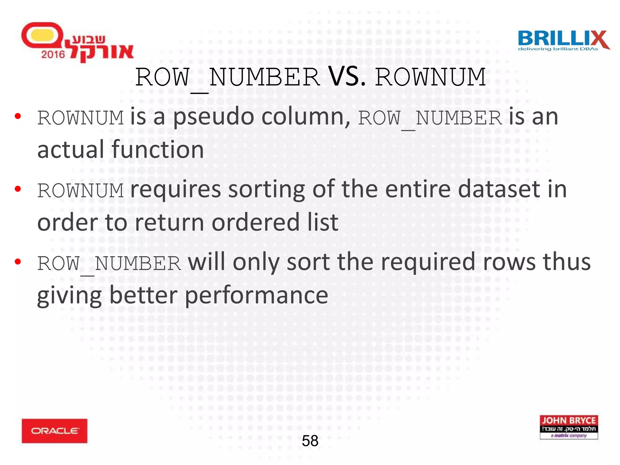
![57 Working with the ROW_NUMBER Function • The ROW_NUMBER function calculates a sequential number of a value in a group of values. • When using the ROW_NUMBER function, ascending is the default sort order, which you can change to descending. • Rows with equal values for the ranking criteria receive a different number. ROW_NUMBER ( ) OVER ( [query_partition_clause] order_by_clause )](https://image.slidesharecdn.com/15102-oracledatabaseadvancedqueryingfinal-161128213310/75/Oracle-Database-Advanced-Querying-2016-52-2048.jpg)
![59 Working With The NTILE Function • Not really a rank function • Divides an ordered data set into a number of buckets indicated by expr and assigns the appropriate bucket number to each row • The buckets are numbered 1 through expr NTILE ( expr ) OVER ([query_partition_clause] order_by_clause)](https://image.slidesharecdn.com/15102-oracledatabaseadvancedqueryingfinal-161128213310/75/Oracle-Database-Advanced-Querying-2016-54-2048.jpg)
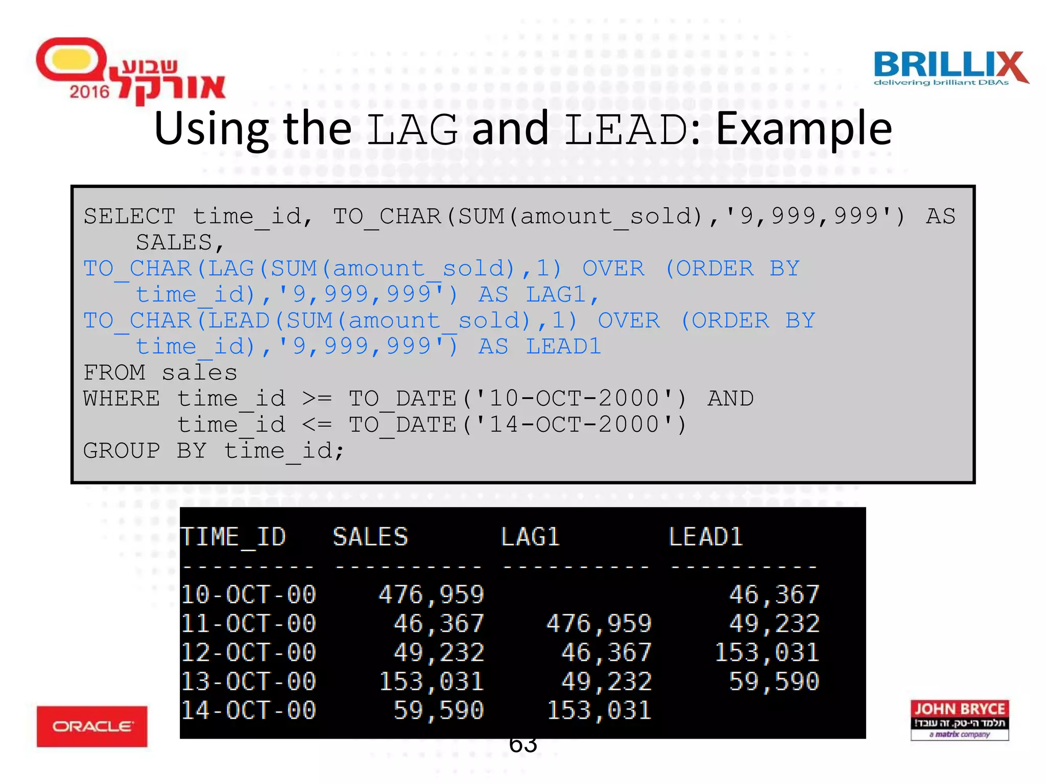
![62 Using the LAG and LEAD Analytic Functions • LAG provides access to more than one row of a table at the same time without a self-join. • Given a series of rows returned from a query and a position of the cursor, LAG provides access to a row at a given physical offset before that position. • If you do not specify the offset, its default is 1. • If the offset goes beyond the scope of the window, the optional default value is returned. If you do not specify the default, its value is NULL. {LAG | LEAD}(value_expr [, offset ] [, default ]) OVER ([ query_partition_clause ] order_by_clause)](https://image.slidesharecdn.com/15102-oracledatabaseadvancedqueryingfinal-161128213310/75/Oracle-Database-Advanced-Querying-2016-57-2048.jpg)
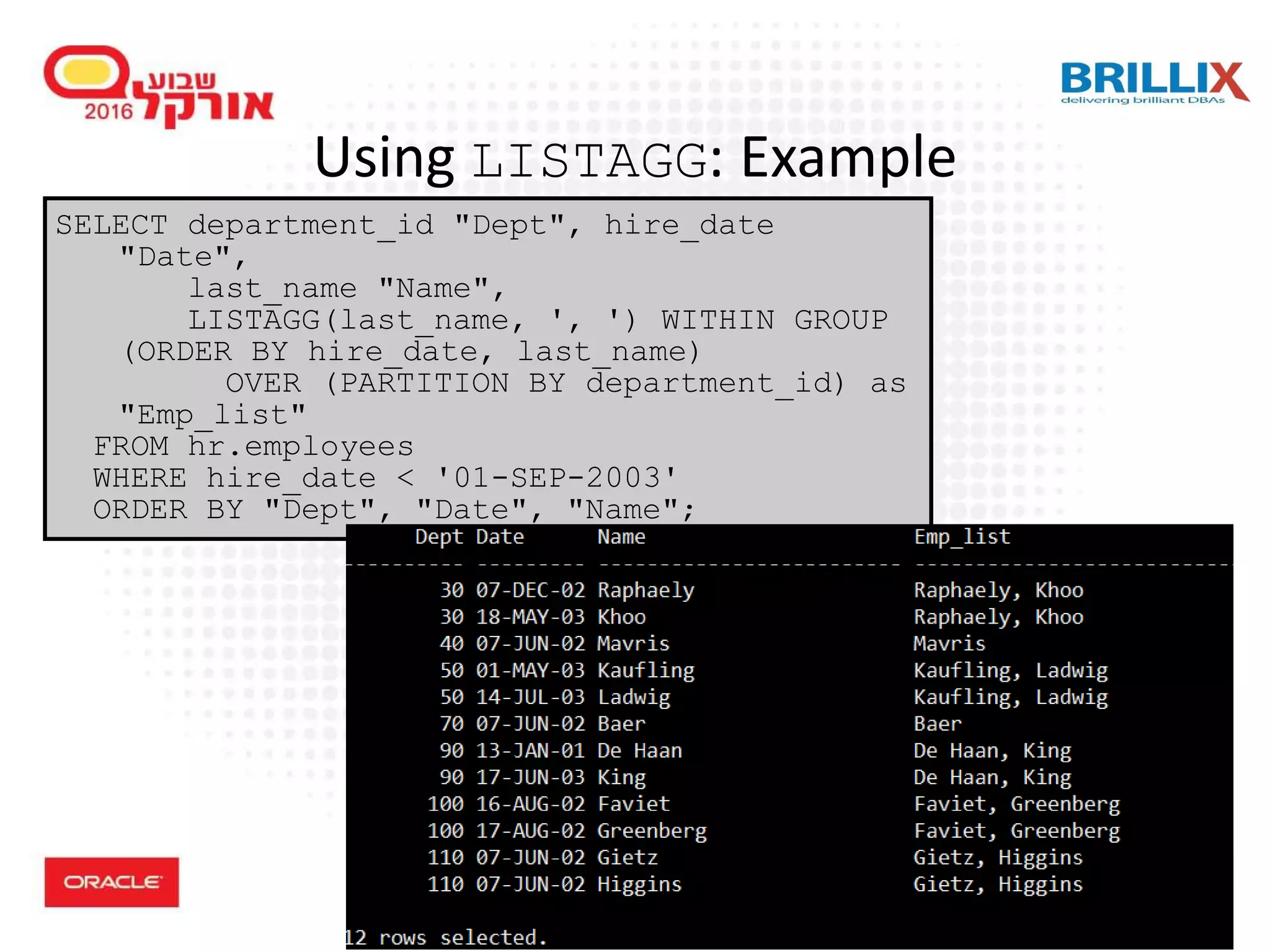
![64 Using the LISTAGG Function • For a specified measure, LISTAGG orders data within each group specified in the ORDER BY clause and then concatenates the values of the measure column LISTAGG(measure_expr [, 'delimiter']) WITHIN GROUP (order_by_clause) [OVER query_partition_clause]](https://image.slidesharecdn.com/15102-oracledatabaseadvancedqueryingfinal-161128213310/75/Oracle-Database-Advanced-Querying-2016-59-2048.jpg)
![66 LISTAGG in Oracle 12c • Limited to output of 4000 chars or 32000 with extended column sizes • Oracle 12cR2 provides overflow handling: • Example: listagg ( measure_expr, ',' [ on overflow (truncate|error) ] [ text ] [ (with|without) count ] ) within group (order by cols) select listagg(table_name, ',' on overflow truncate) within group (order by table_name) table_names from dba_tables](https://image.slidesharecdn.com/15102-oracledatabaseadvancedqueryingfinal-161128213310/75/Oracle-Database-Advanced-Querying-2016-61-2048.jpg)
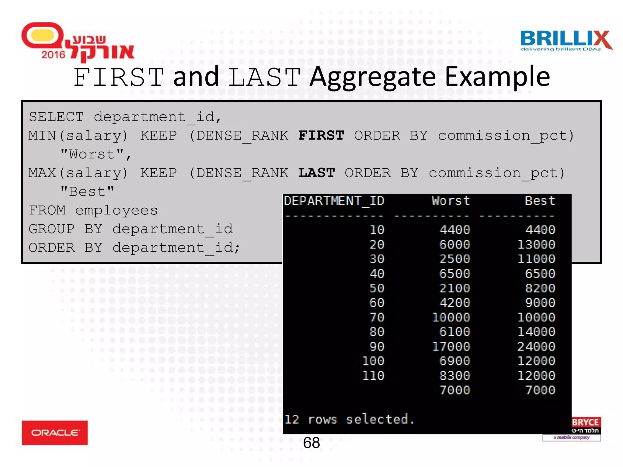
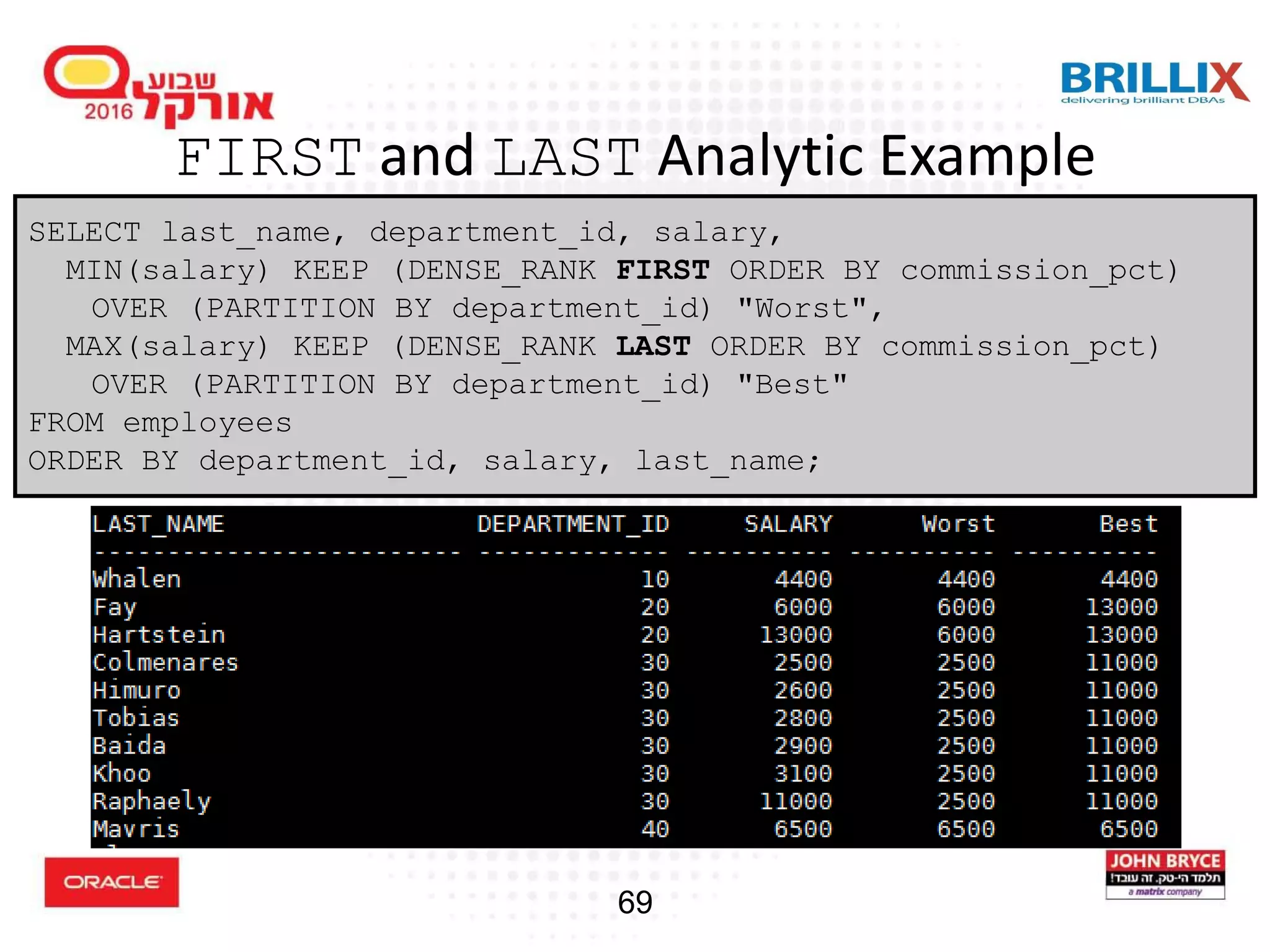
![67 Using the FIRST and LAST Functions • Both are aggregate and analytic functions • Used to retrieve a value from the first or last row of a sorted group, but the needed value is not the sort key • FIRST and LAST functions eliminate the need for self- joins or views and enable better performance aggregate_function KEEP (DENSE_RANK FIRST ORDER BY expr [ DESC | ASC ][ NULLS { FIRST | LAST } ] [, expr [ DESC | ASC ] [ NULLS { FIRST | LAST } ] ]... ) [ OVER query_partition_clause ]](https://image.slidesharecdn.com/15102-oracledatabaseadvancedqueryingfinal-161128213310/75/Oracle-Database-Advanced-Querying-2016-62-2048.jpg)
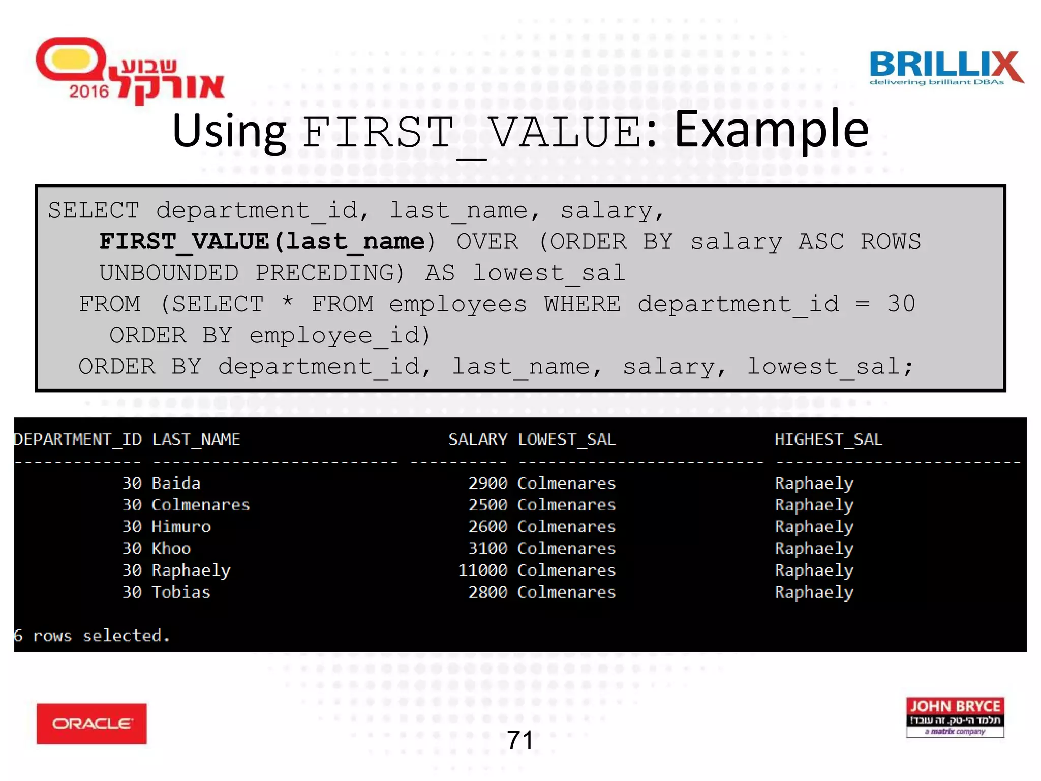
![70 Using FIRST_VALUE Analytic Function • Returns the first value in an ordered set of values • If the first value in the set is null, then the function returns NULL unless you specify IGNORE NULLS. This setting is useful for data densification. FIRST_VALUE (expr [ IGNORE NULLS ]) OVER (analytic_clause)](https://image.slidesharecdn.com/15102-oracledatabaseadvancedqueryingfinal-161128213310/75/Oracle-Database-Advanced-Querying-2016-65-2048.jpg)
![72 Using LAST_VALUE Analytic Function • Returns the last value in an ordered set of values. LAST_VALUE (expr [ IGNORE NULLS ]) OVER (analytic_clause)](https://image.slidesharecdn.com/15102-oracledatabaseadvancedqueryingfinal-161128213310/75/Oracle-Database-Advanced-Querying-2016-67-2048.jpg)
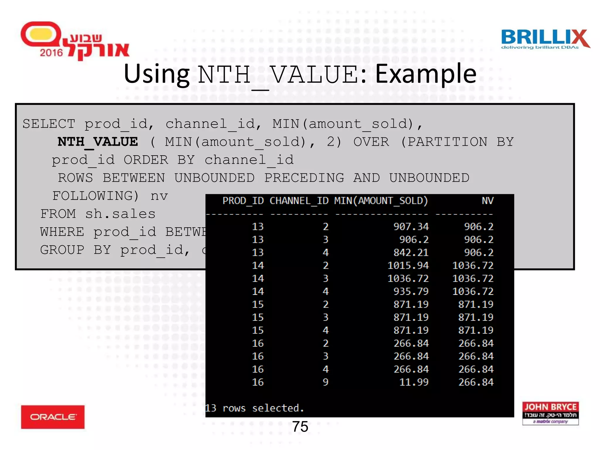
![73 Using NTH_VALUE Analytic Function • Returns the N-th values in an ordered set of values • Different default window: RANGE BETWEEN UNBOUNDED PRECEDING AND CURRENT ROW NTH_VALUE (measure_expr, n) [ FROM { FIRST | LAST } ][ { RESPECT | IGNORE } NULLS ] OVER (analytic_clause)](https://image.slidesharecdn.com/15102-oracledatabaseadvancedqueryingfinal-161128213310/75/Oracle-Database-Advanced-Querying-2016-68-2048.jpg)


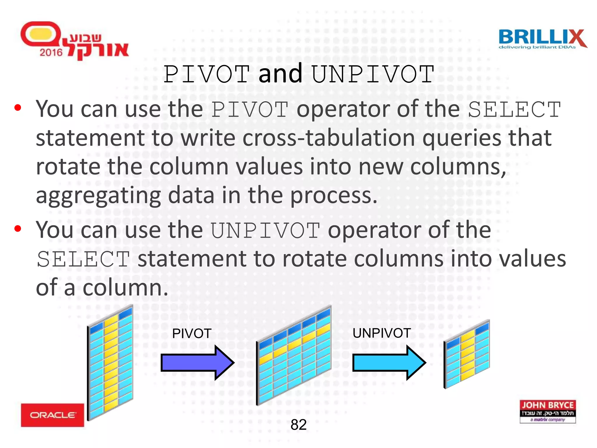
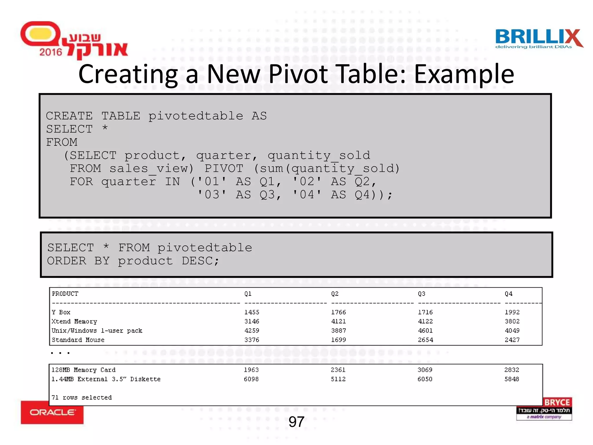
![85 PIVOT Clause Syntax table_reference PIVOT [ XML ] ( aggregate_function ( expr ) [[AS] alias ] [, aggregate_function ( expr ) [[AS] alias ] ]... pivot_for_clause pivot_in_clause ) -- Specify the column(s) to pivot whose values are to -- be pivoted into columns. pivot_for_clause = FOR { column |( column [, column]... ) } -- Specify the pivot column values from the columns you -- specified in the pivot_for_clause. pivot_in_clause = IN ( { { { expr | ( expr [, expr]... ) } [ [ AS] alias] }... | subquery | { ANY | ANY [, ANY]...} } )](https://image.slidesharecdn.com/15102-oracledatabaseadvancedqueryingfinal-161128213310/75/Oracle-Database-Advanced-Querying-2016-80-2048.jpg)


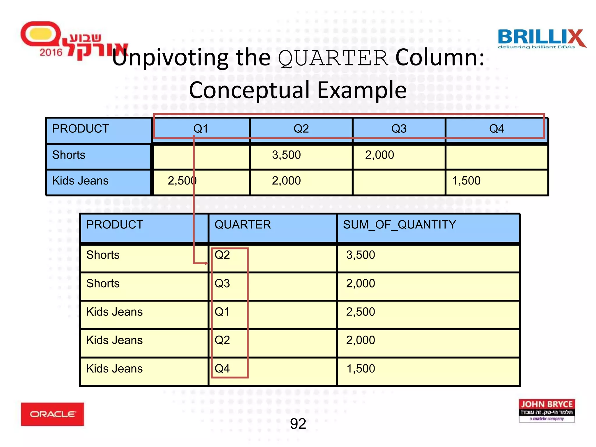
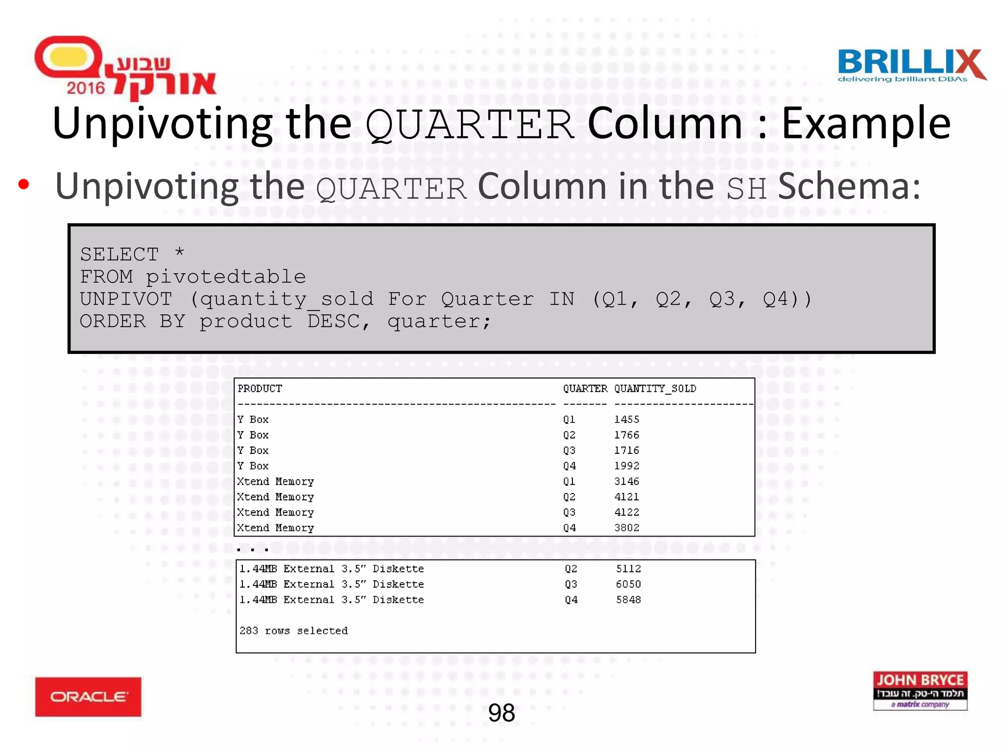
![96 UNPIVOT Clause Syntax table_reference UNPIVOT [{INCLUDE|EXCLUDE} NULLS] -- specify the measure column(s) to be unpivoted. ( { column | ( column [, column]... ) } unpivot_for_clause unpivot_in_clause ) -- Specify one or more names for the columns that will -- result from the unpivot operation. unpivot_for_clause = FOR { column | ( column [, column]... ) } -- Specify the columns that will be unpivoted into values of -- the column specified in the unpivot_for_clause. unpivot_in_clause = ( { column | ( column [, column]... ) } [ AS { constant | ( constant [, constant]... ) } ] [, { column | ( column [, column]... ) } [ AS { constant | ( constant [, constant]...) } ] ]...)](https://image.slidesharecdn.com/15102-oracledatabaseadvancedqueryingfinal-161128213310/75/Oracle-Database-Advanced-Querying-2016-88-2048.jpg)

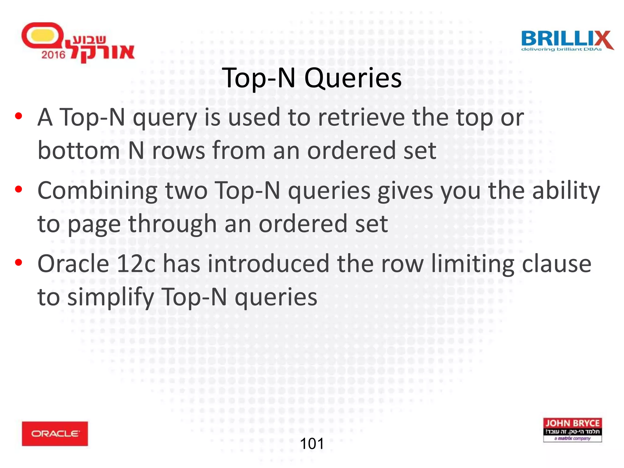
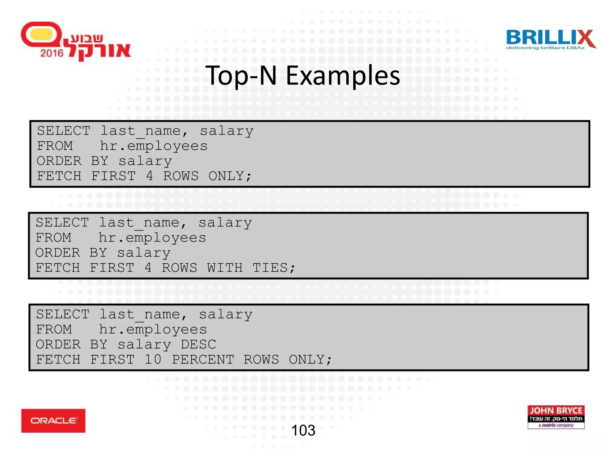
![102 Top-N in 12cR1 • This is ANSI syntax • The default offset is 0 • Null values in offset, rowcount or percent will return no rows [ OFFSET offset { ROW | ROWS } ] [ FETCH { FIRST | NEXT } [ { rowcount | percent PERCENT } ] { ROW | ROWS } { ONLY | WITH TIES } ]](https://image.slidesharecdn.com/15102-oracledatabaseadvancedqueryingfinal-161128213310/75/Oracle-Database-Advanced-Querying-2016-94-2048.jpg)


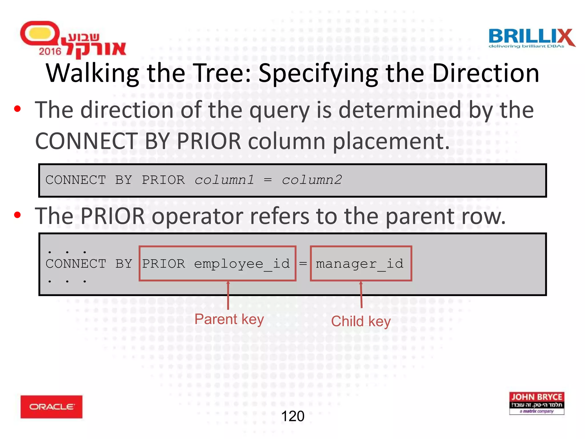
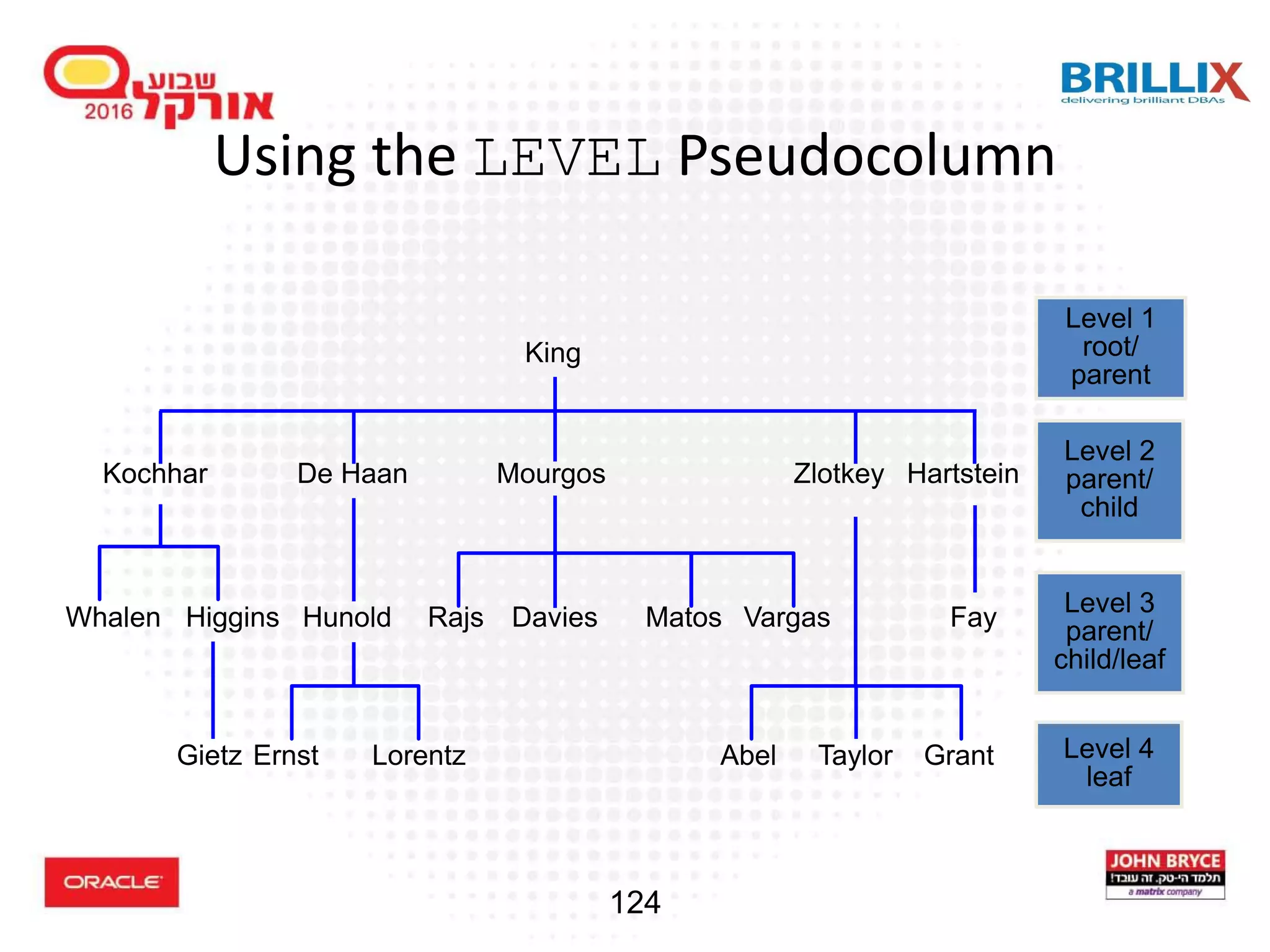
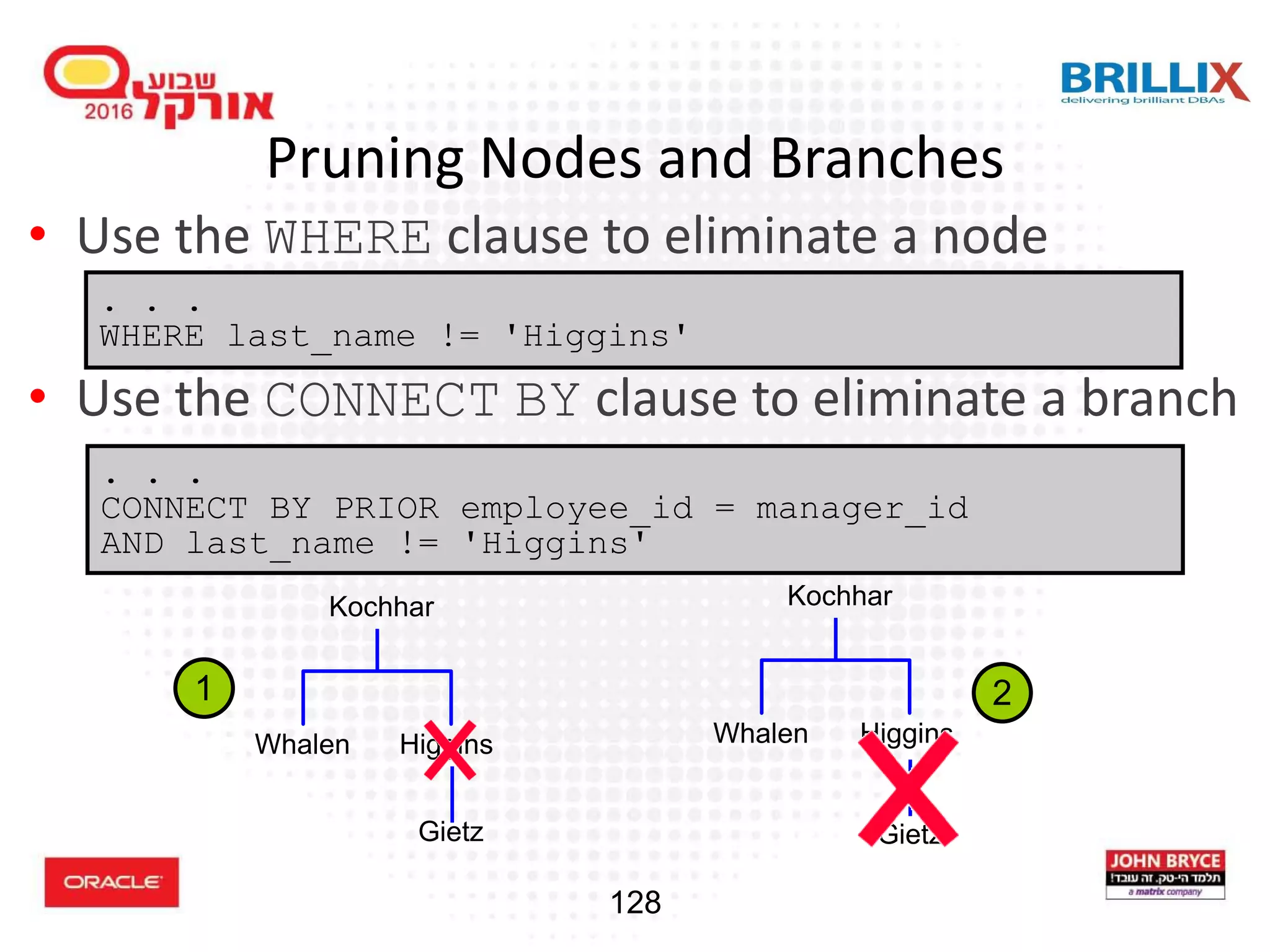
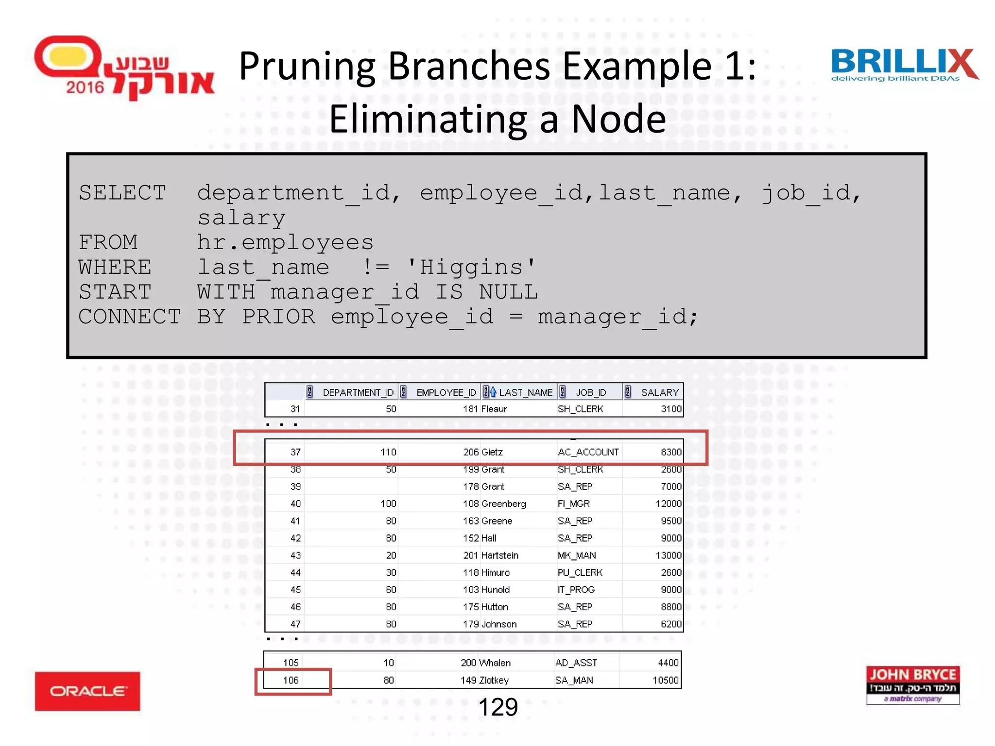
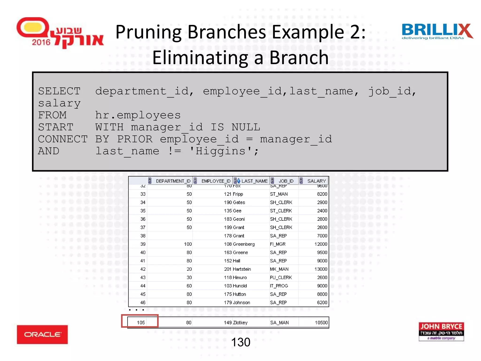
![118 Hierarchical Queries: Syntax • condition: expr comparison_operator expr SELECT [LEVEL], column, expr... FROM table [WHERE condition(s)] [START WITH condition(s)] [CONNECT BY PRIOR condition(s)] ;](https://image.slidesharecdn.com/15102-oracledatabaseadvancedqueryingfinal-161128213310/75/Oracle-Database-Advanced-Querying-2016-110-2048.jpg)

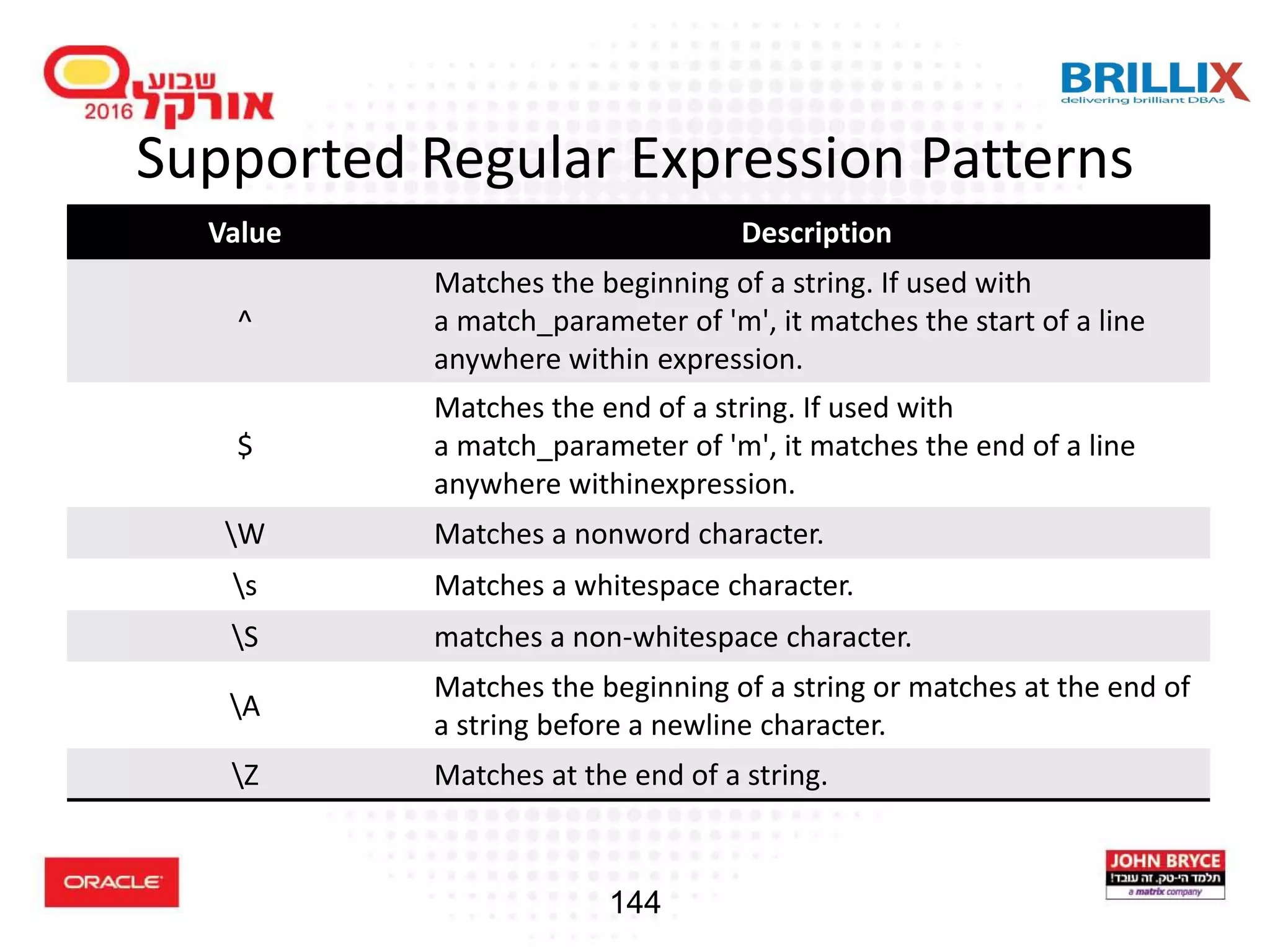
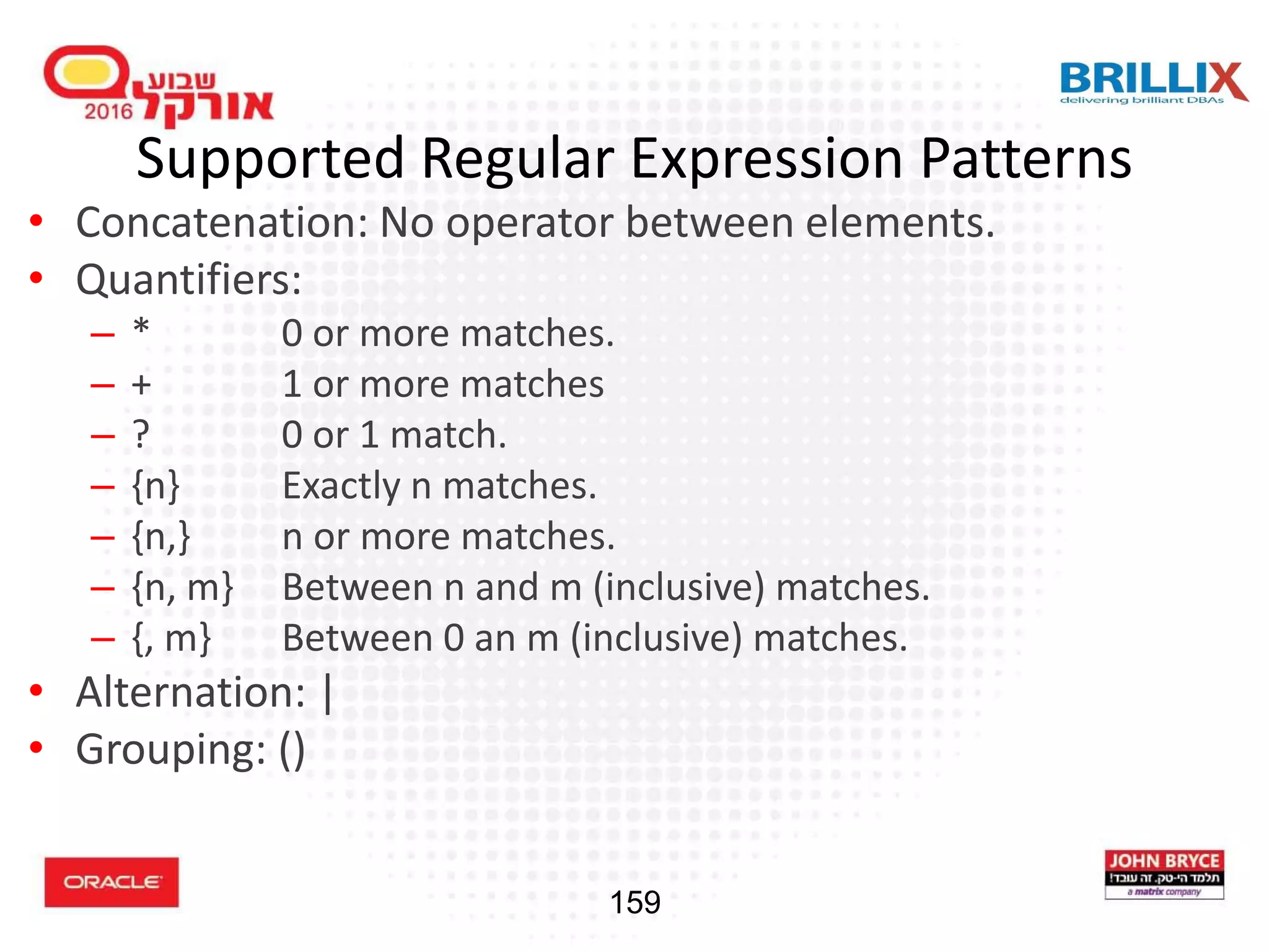
![143 Supported Regular Expression Patterns • Concatenation: No operator between elements. • Quantifiers: – . Matches any character in the database character set – * 0 or more matches – + 1 or more matches – ? 0 or 1 match – {n} Exactly n matches – {n,} n or more matches – {n, m} Between n and m (inclusive) matches – {, m} Between 0 an m (inclusive) matches • Alternation: [|] • Grouping: ()](https://image.slidesharecdn.com/15102-oracledatabaseadvancedqueryingfinal-161128213310/75/Oracle-Database-Advanced-Querying-2016-131-2048.jpg)
![145 Character Classes Character Class Description [:alnum:] Alphanumeric characters [:alpha:] Alphabetic characters [:blank:] Blank Space Characters [:cntrl:] Control characters (nonprinting) [:digit:] Numeric digits [:graph:] Any [:punct:], [:upper:], [:lower:], and [:digit:] chars [:lower:] Lowercase alphabetic characters [:print:] Printable characters [:punct:] Punctuation characters [:space:] Space characters (nonprinting), such as carriage return, newline, vertical tab, and form feed [:upper:] Uppercase alphabetic characters [:xdigit:] Hexidecimal characters](https://image.slidesharecdn.com/15102-oracledatabaseadvancedqueryingfinal-161128213310/75/Oracle-Database-Advanced-Querying-2016-133-2048.jpg)


![151 MATCH_RECOGNIZE Syntax SELECT FROM [row pattern input table] MATCH_RECOGNIZE` ( [ PARTITION BY <cols> ] [ ORDER BY <cols> ] [ MEASURES <cols> ] [ ONE ROW PER MATCH | ALL ROWS PER MATCH ] [ SKIP_TO_option] PATTERN ( <row pattern> ) DEFINE <definition list> )](https://image.slidesharecdn.com/15102-oracledatabaseadvancedqueryingfinal-161128213310/75/Oracle-Database-Advanced-Querying-2016-139-2048.jpg)


![172 Example of Using DBMS_XMLGEN select dbms_xmlgen.getxml(q'{ select column_name, data_type from all_tab_columns where table_name = 'EMPLOYEES' and owner = 'HR'}') from dual / <?xml version="1.0"?> <ROWSET> <ROW> <COLUMN_NAME>EMPLOYEE_ID</COLUMN_NAME> <DATA_TYPE>NUMBER</DATA_TYPE> </ROW> <ROW> <COLUMN_NAME>FIRST_NAME</COLUMN_NAME> <DATA_TYPE>VARCHAR2</DATA_TYPE> </ROW> [...] </ROWSET>](https://image.slidesharecdn.com/15102-oracledatabaseadvancedqueryingfinal-161128213310/75/Oracle-Database-Advanced-Querying-2016-160-2048.jpg)


![189 What is JSON • JavaScript Object Notation • Converts database tables to a readable document – just like XML but simpler • Very common in NoSQL and Big Data solutions {"FirstName" : "Zohar", "LastName" : "Elkayam", "Age" : 36, "Connection" : [ {"Type" : “Email", "Value" : "zohar@DBAces.com"}, {"Type" : “Twitter", "Value" : “@realmgic"}, {"Type" : "Site", "Value" : "www.realdbamagic.com"}, ]}](https://image.slidesharecdn.com/15102-oracledatabaseadvancedqueryingfinal-161128213310/75/Oracle-Database-Advanced-Querying-2016-177-2048.jpg)
![193 JSON Path Expression • Similar role to XPATH in XML • Syntactically similar to Java Script (. and [ ]) • Compatible with Java Script](https://image.slidesharecdn.com/15102-oracledatabaseadvancedqueryingfinal-161128213310/75/Oracle-Database-Advanced-Querying-2016-181-2048.jpg)

![198 Example: JSON_TABLE (2) • 1 row output for each member of LineItems array select D.* from J_PURCHASEORDER p, JSON_TABLE( p.PO_DOCUMENT, '$' columns( PO_NUMBER NUMBER(10) path '$.PONumber', NESTED PATH '$.LineItems[*]' columns( ITEMNO NUMBER(16) path '$.ItemNumber', UPCCODE VARCHAR2(14 CHAR) path '$.Part.UPCCode‘ )) ) D where PO_NUMBER = 1600 or PO_NUMBER = 1601 /](https://image.slidesharecdn.com/15102-oracledatabaseadvancedqueryingfinal-161128213310/75/Oracle-Database-Advanced-Querying-2016-186-2048.jpg)
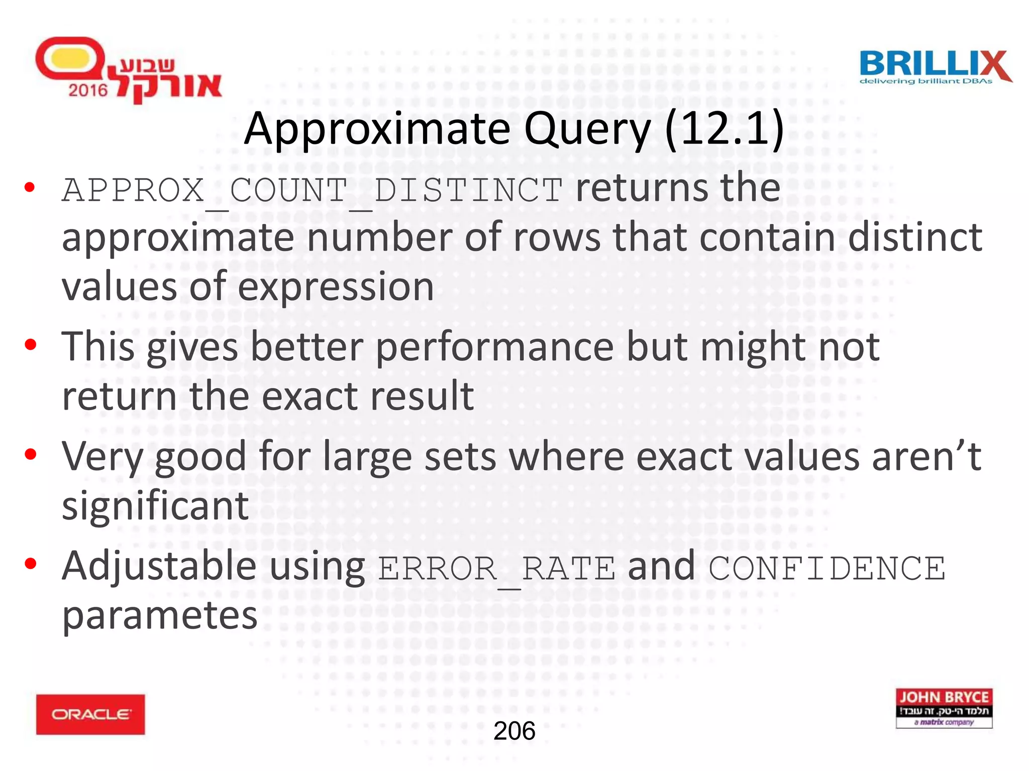
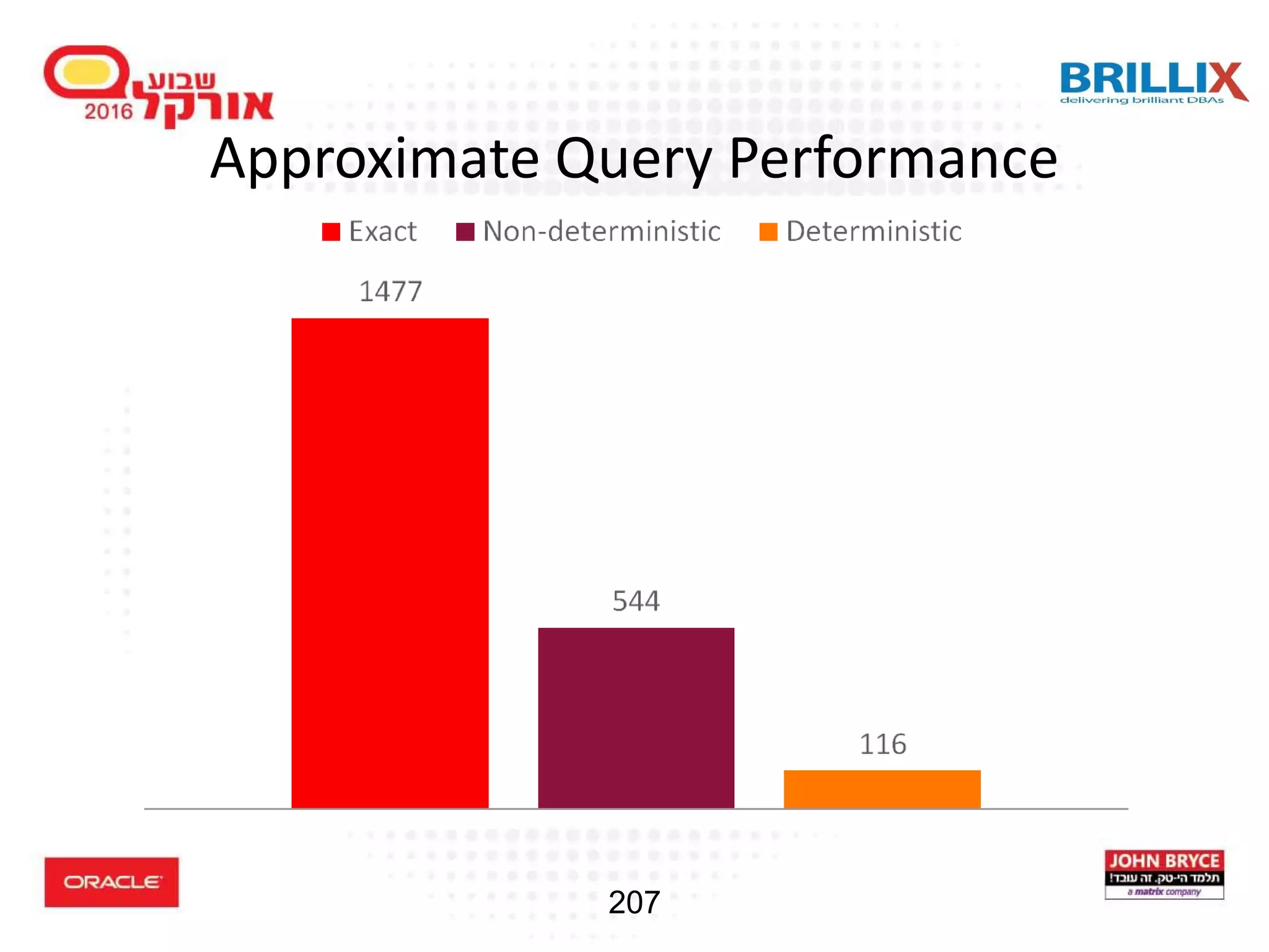
![208 Approximate Query Enhancements (12.2) • 12.2 introduced a parameter, approx_for_count_distinct which automatically replace count distinct with APPROX_COUNT_DISTINCT • New approximate function: approx_percentile approx_percentile ( <expression> [ deterministic ], [ ('ERROR_RATE' | 'CONFIDENCE') ] ) within group ( order by <expression>)](https://image.slidesharecdn.com/15102-oracledatabaseadvancedqueryingfinal-161128213310/75/Oracle-Database-Advanced-Querying-2016-196-2048.jpg)


![221 Command History • 100 command history buffer • Commands are persistent between sessions (watch out for security!) • Use UP and DOWN arrow keys to access old commands • Usage: history history usage History script history full History clear [session?] • Load from history into command buffer: history <number>](https://image.slidesharecdn.com/15102-oracledatabaseadvancedqueryingfinal-161128213310/75/Oracle-Database-Advanced-Querying-2016-209-2048.jpg)
![228 Load Data From CSV File • Loads a comma separated value (csv) file into a table • The first row of the file must be a header row and the file must be encoded UTF8 • The load is processed with 50 rows per batch • Usage: LOAD [schema.]table_name[@db_link] file_name](https://image.slidesharecdn.com/15102-oracledatabaseadvancedqueryingfinal-161128213310/75/Oracle-Database-Advanced-Querying-2016-216-2048.jpg)


The document outlines an Oracle Database seminar conducted by Zohar Elkayam, CTO of Brillix, covering advanced SQL techniques and new features in Oracle 12c. Key topics include aggregative group functions, analytic functions, and the use of rollup and cube in SQL queries. The seminar aims to enhance participants' SQL skills and familiarize them with analytical processing capabilities and syntax in Oracle SQL.
Overview of the presentation on Oracle Database advanced querying techniques by Zohar Elkayam, CTO at Brillix.
Brillix's services and the agenda covering SQL techniques, analytics, XML, JSON, and new features in Oracle 12c.
Aiming to learn new SQL techniques and explore Oracle 12c features as a foundation for practical applications.
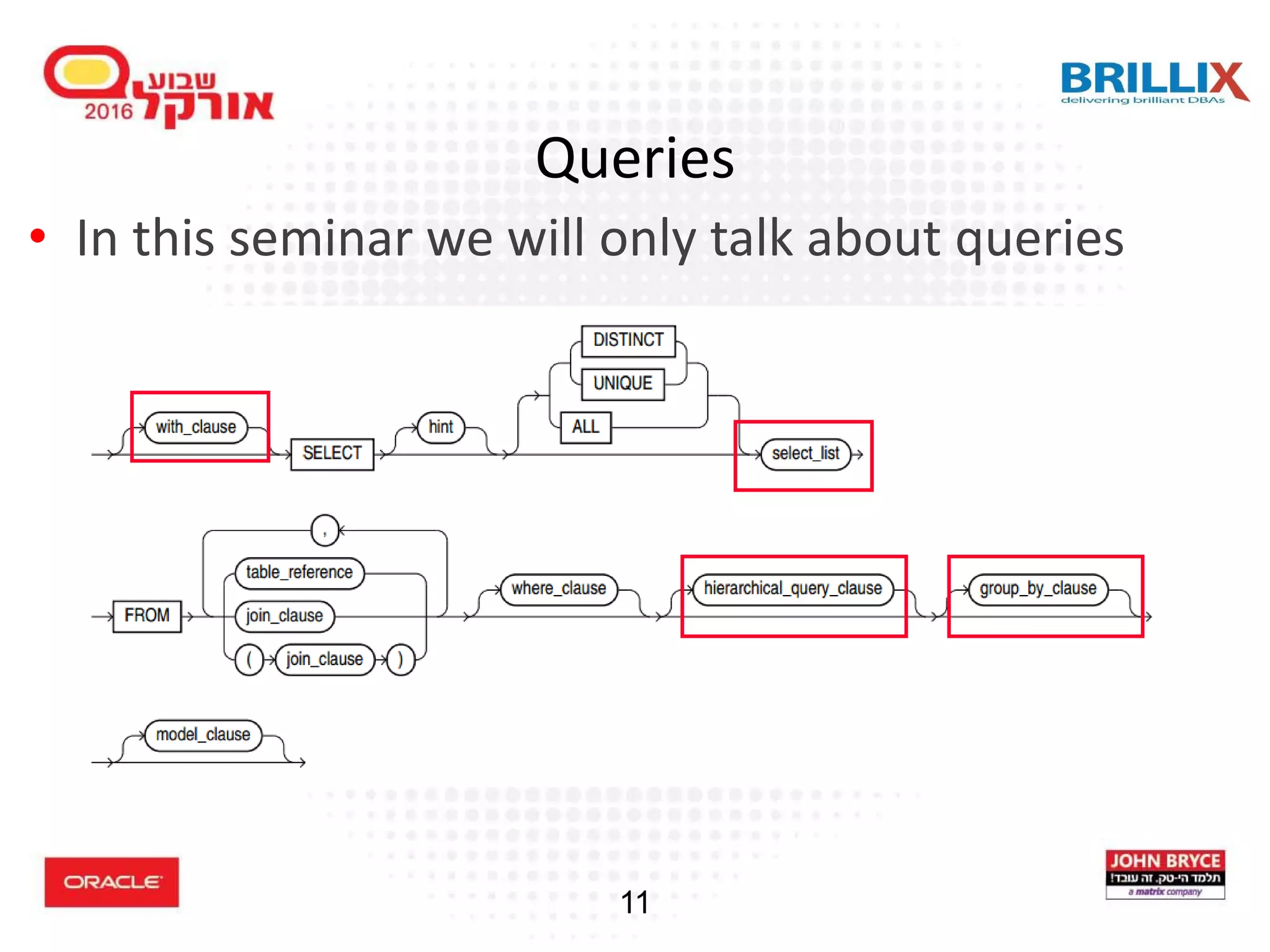
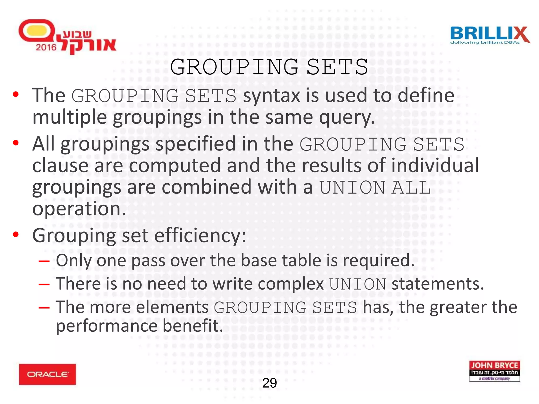
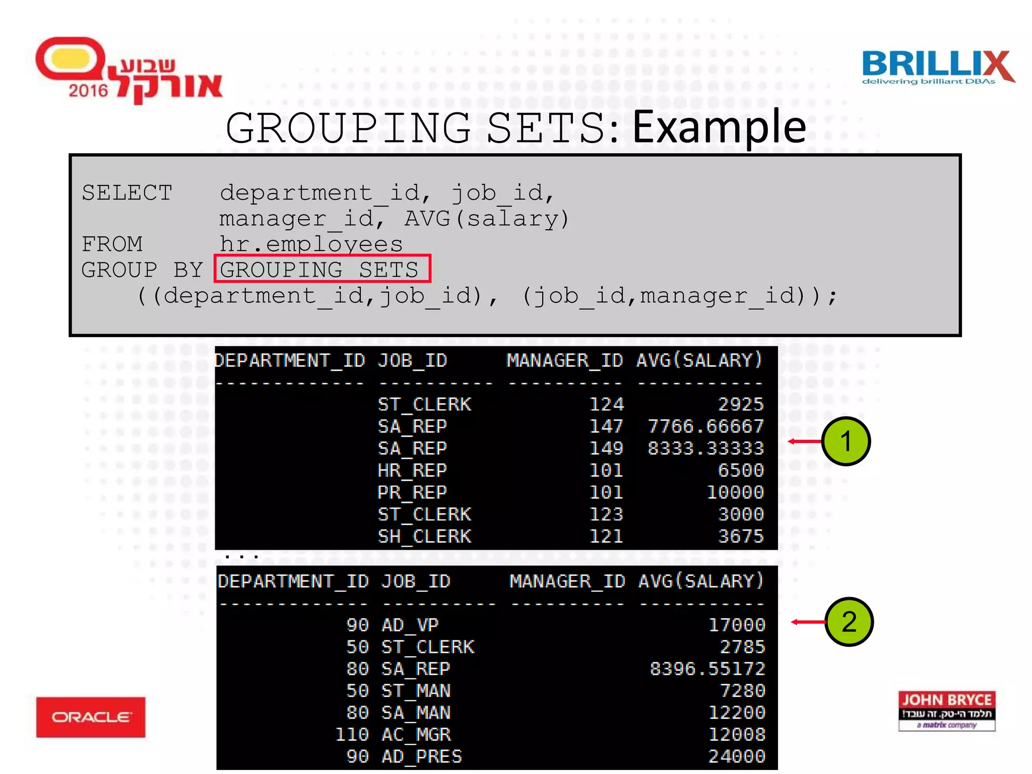
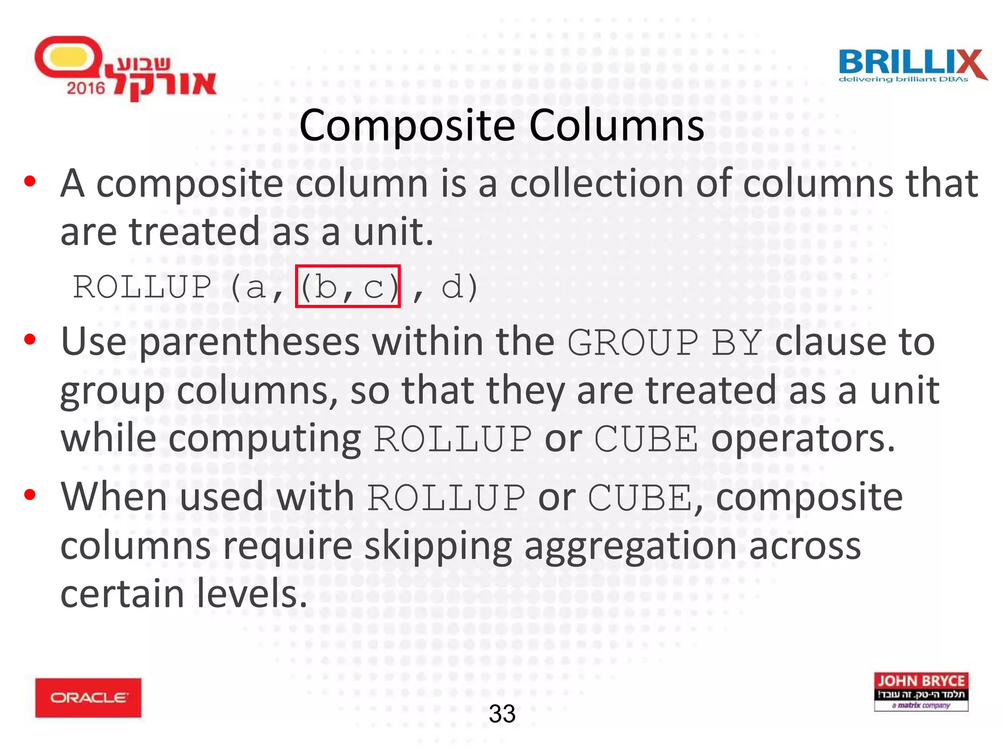
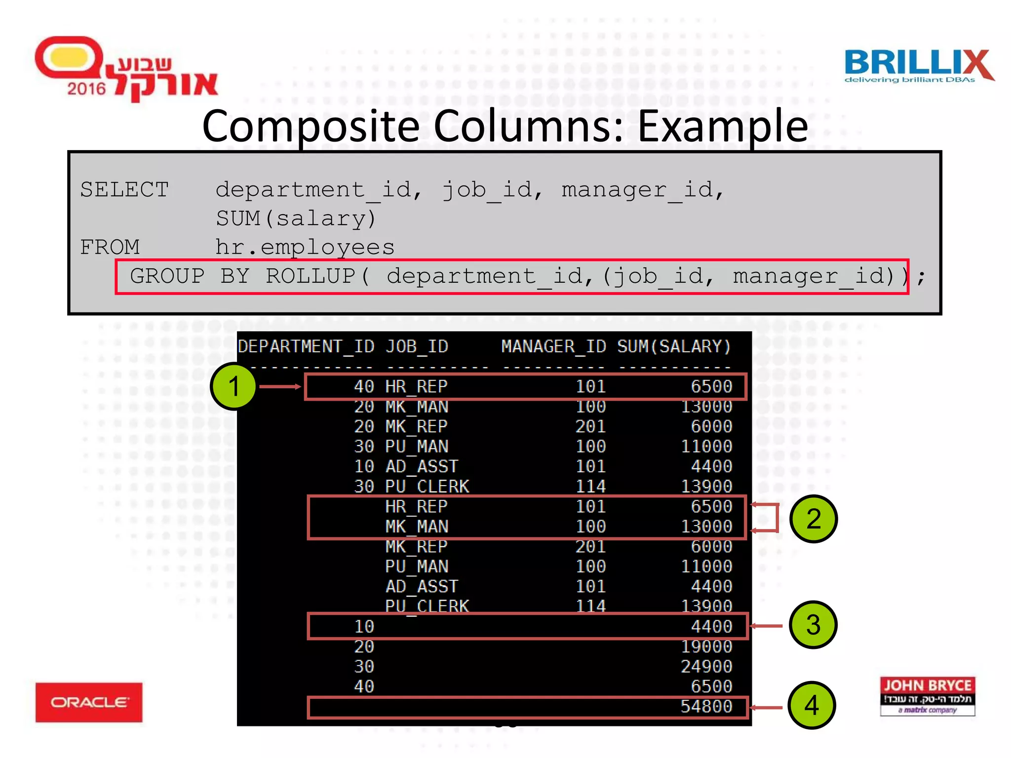
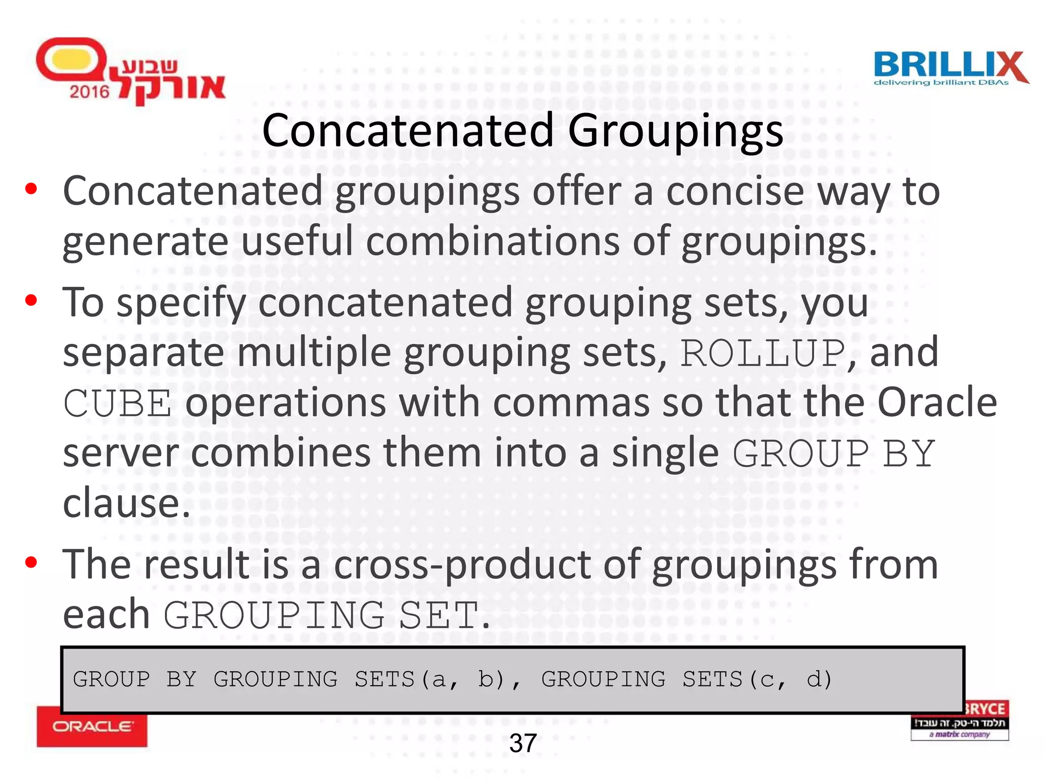
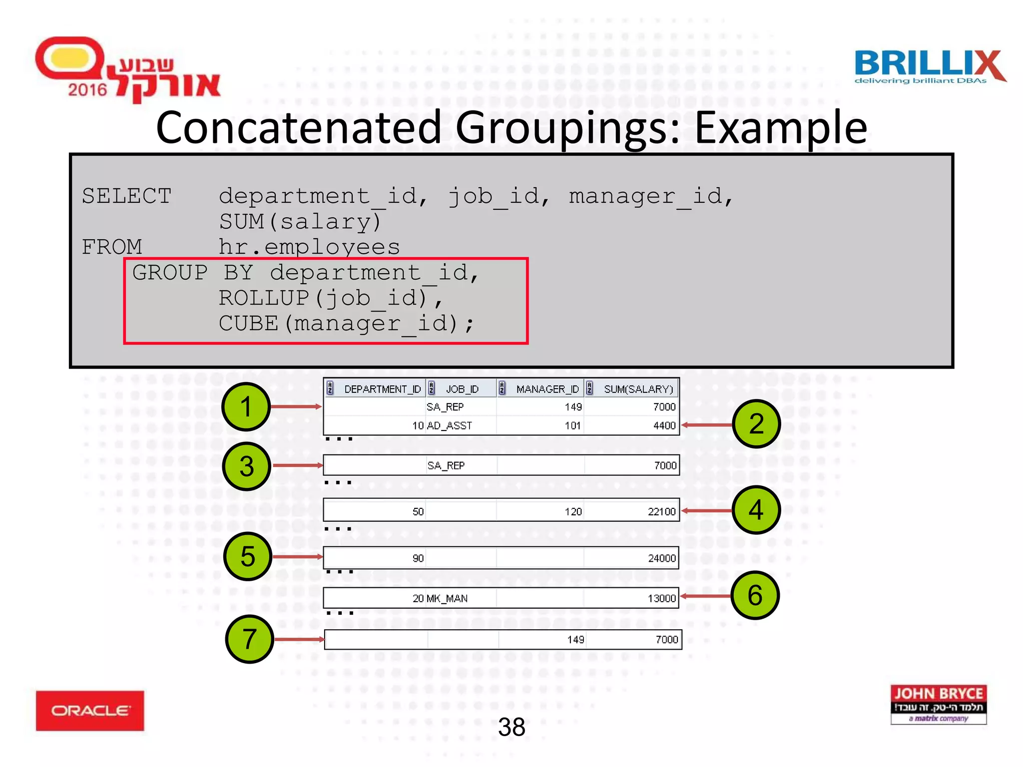
Introduction to SQL, focusing on queries and group functions such as CUBE, ROLLUP, and GROUPING.
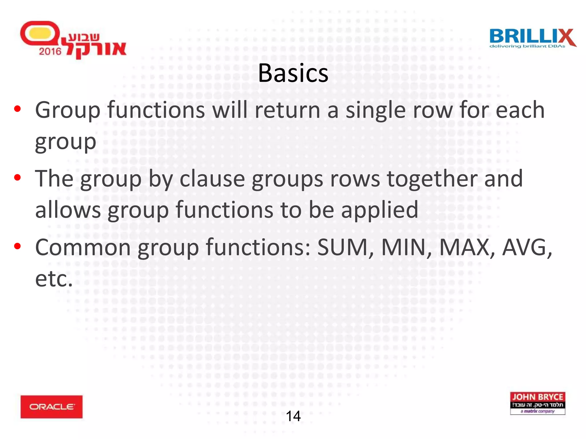
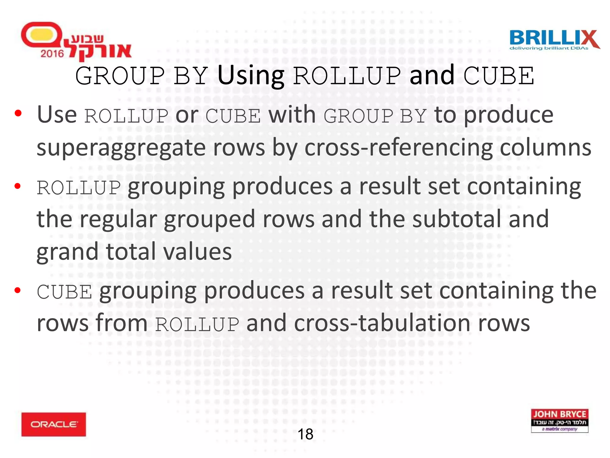
Detailed explanation of group functions, including syntax, examples for GROUP BY, ROLLUP, and CUBE operators.
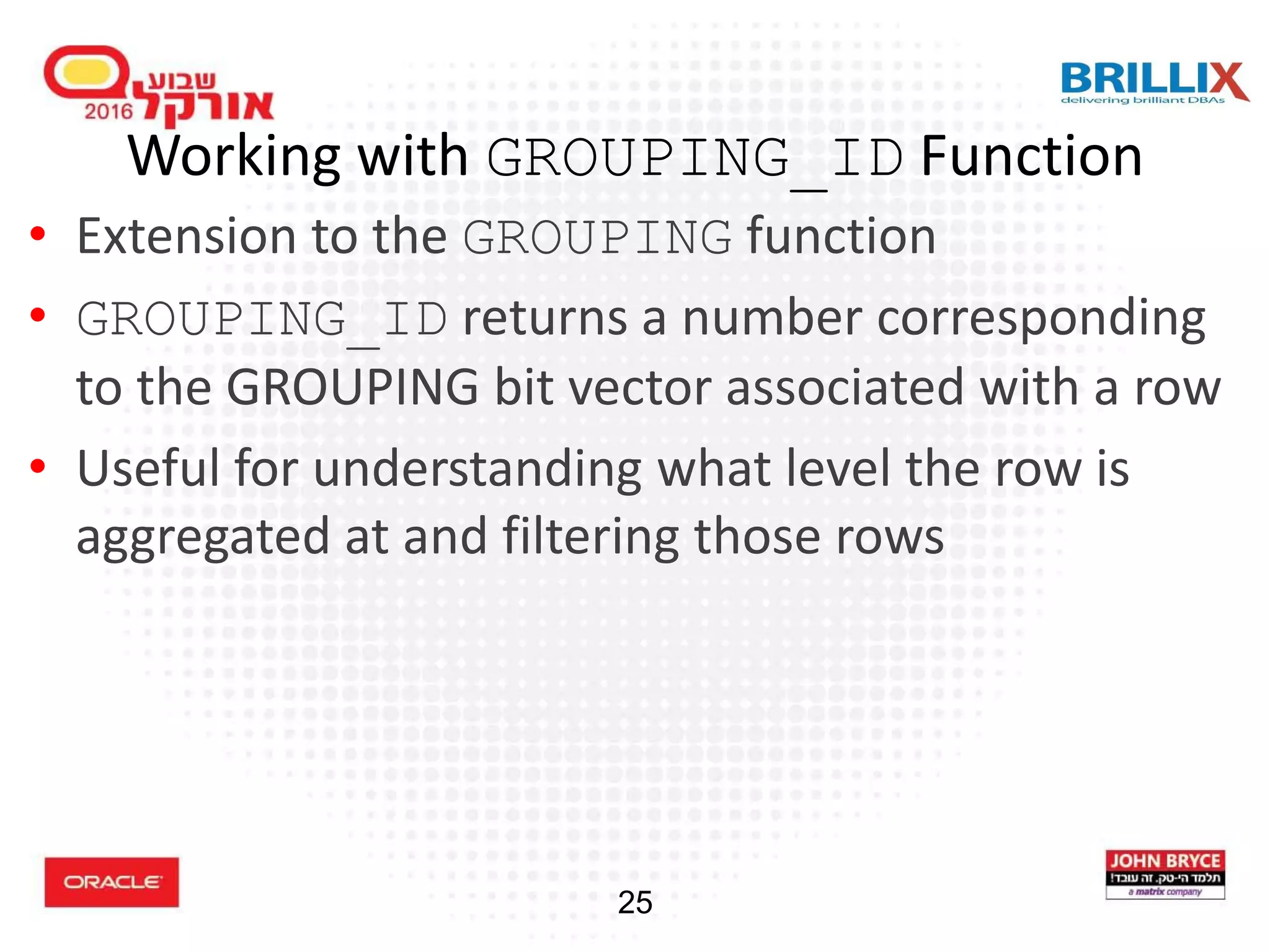
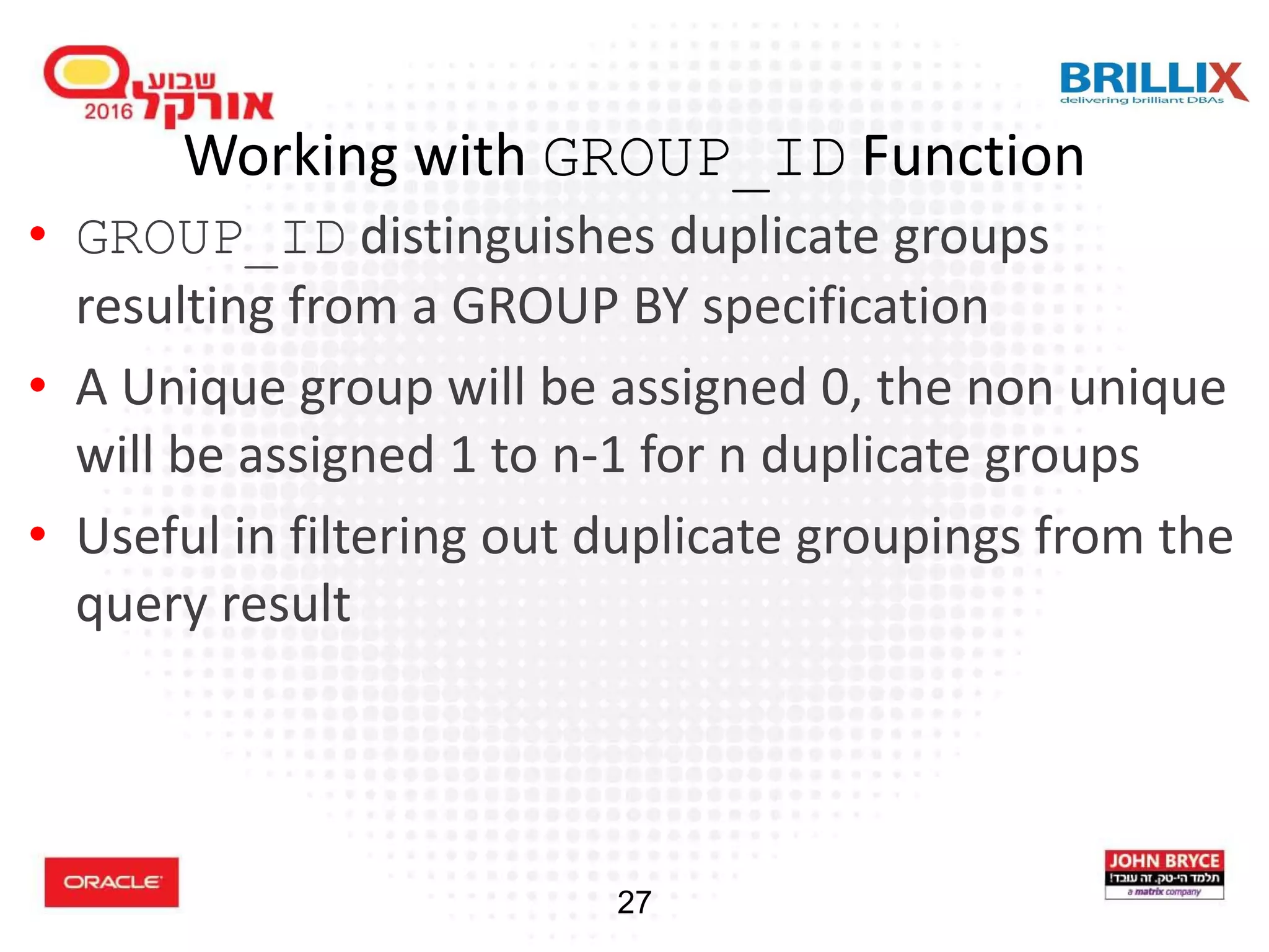
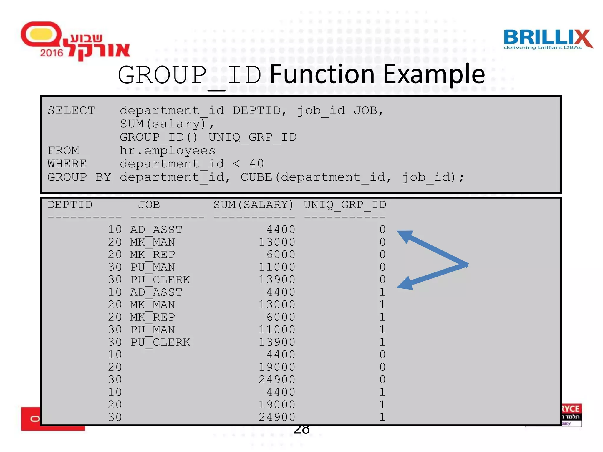
Working with GROUPING functions and GROUPING_ID to understand data levels and filter results.
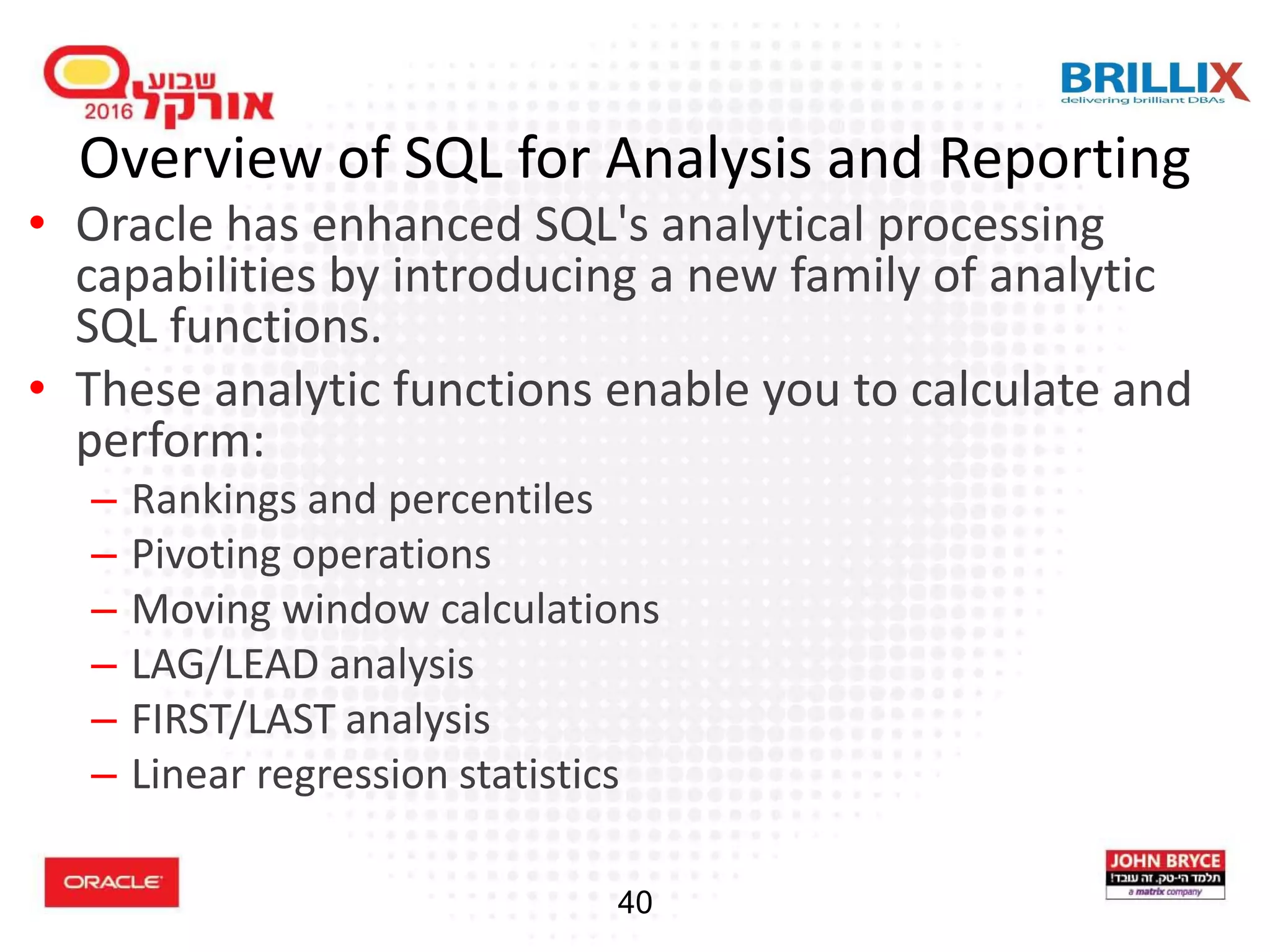
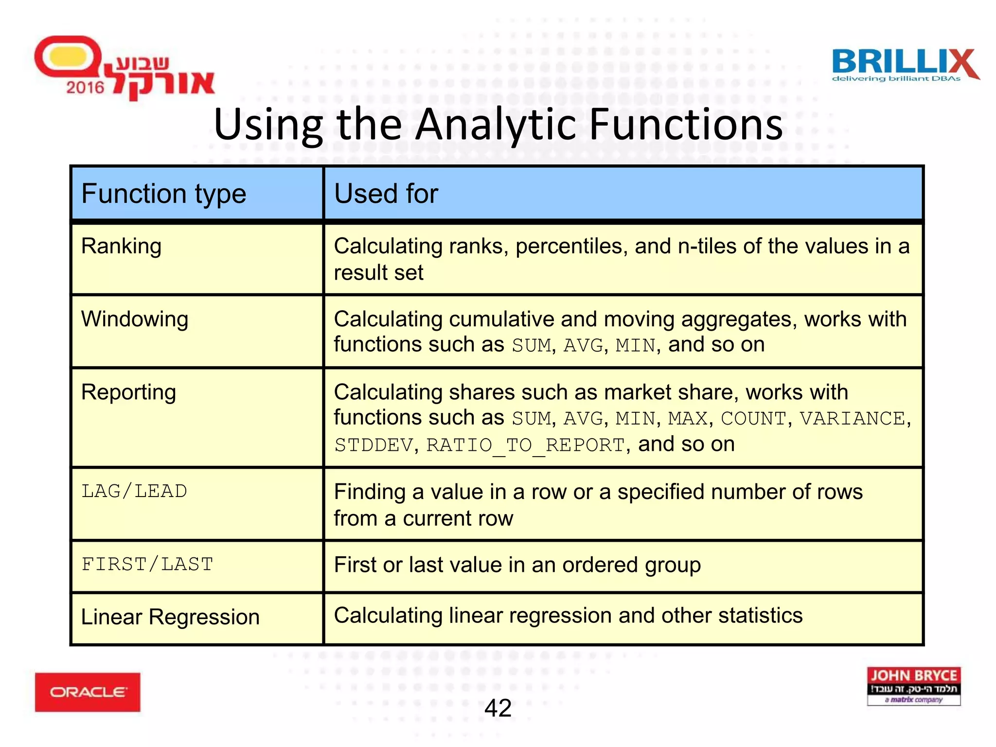
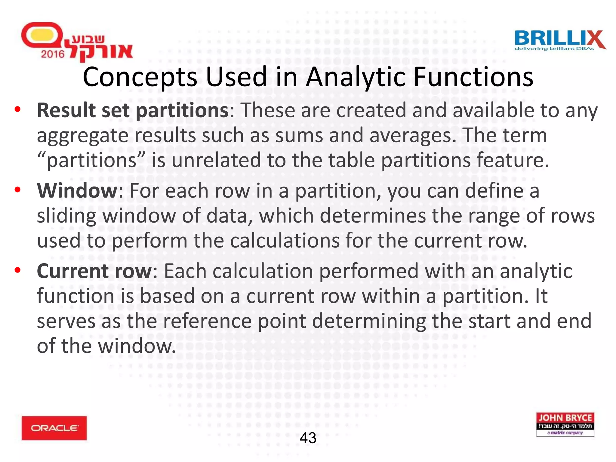
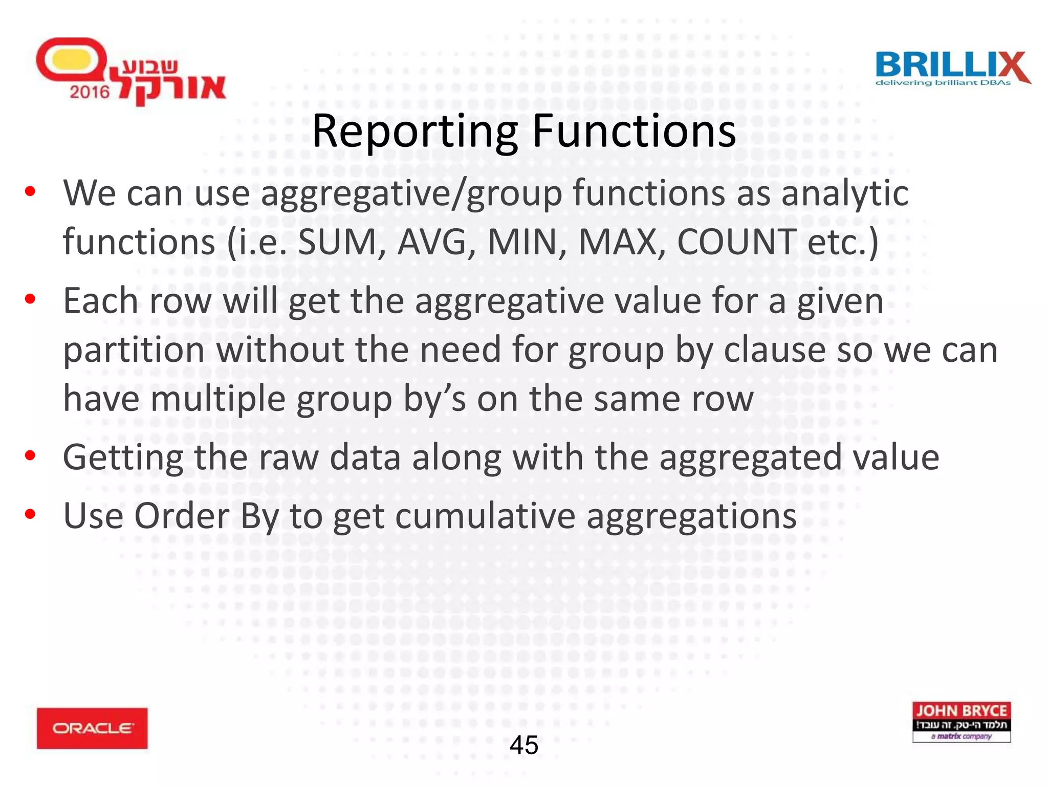
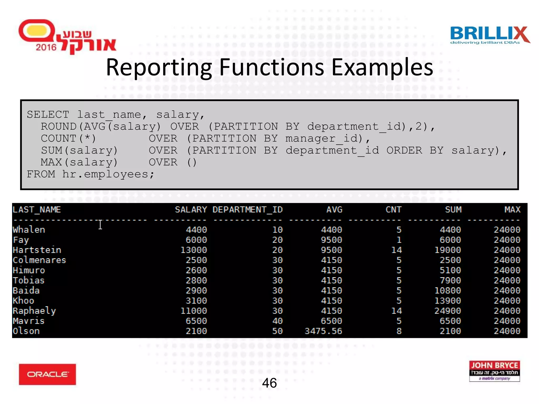
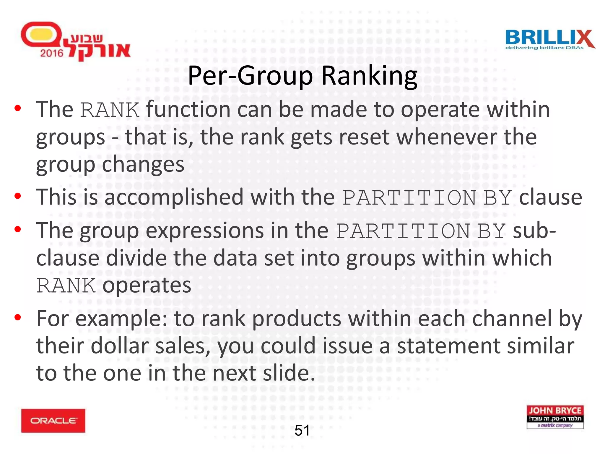
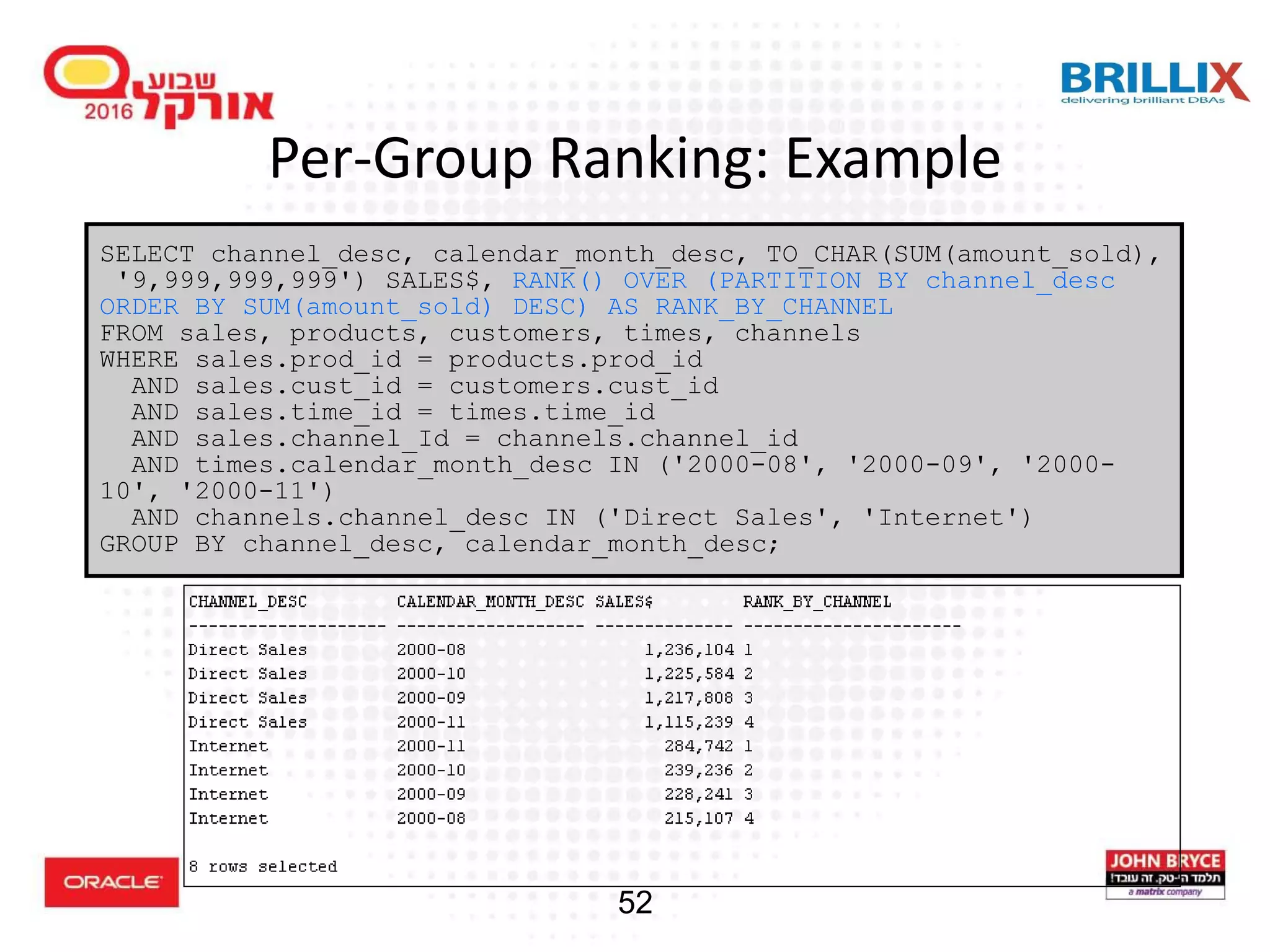
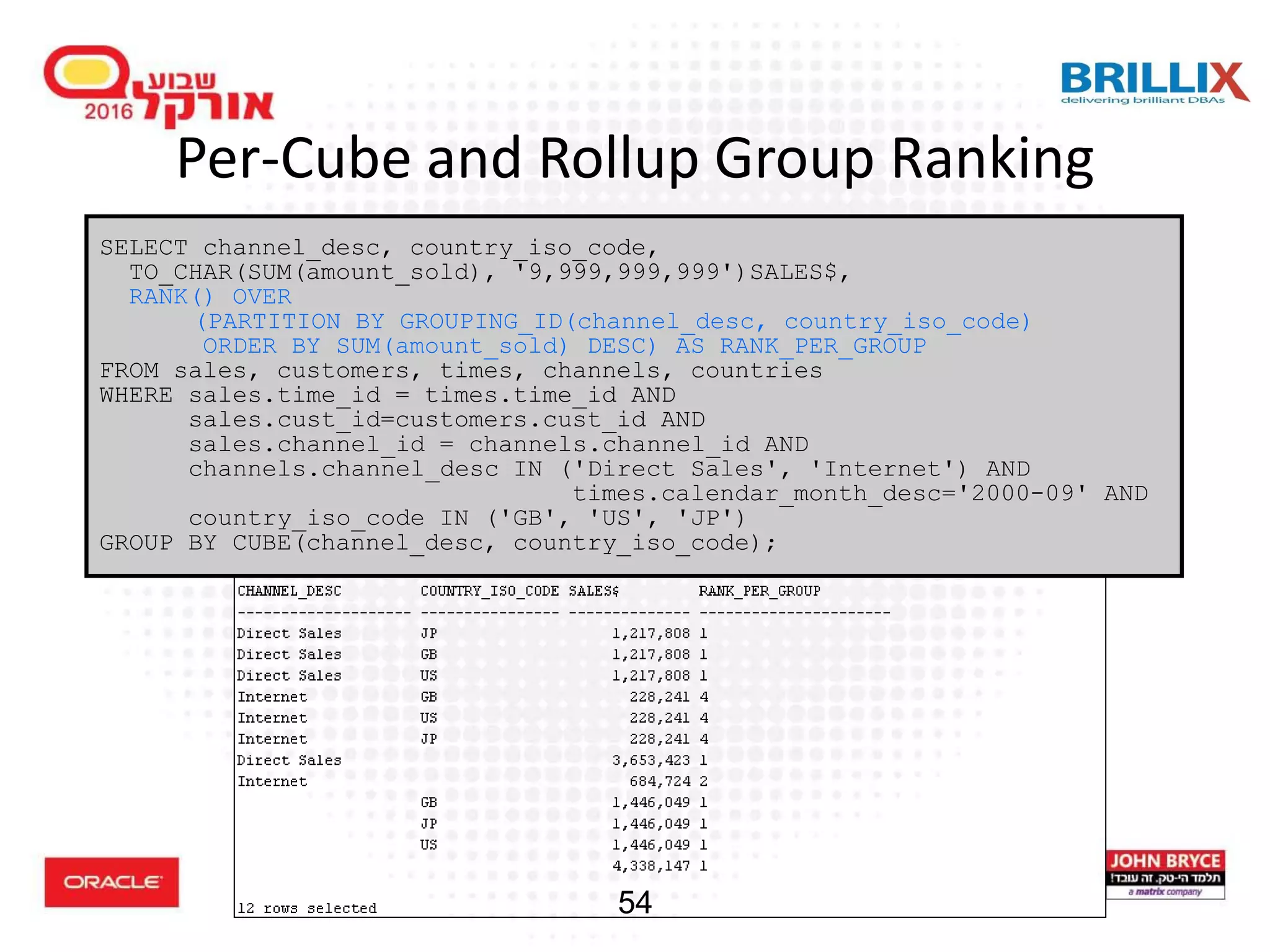
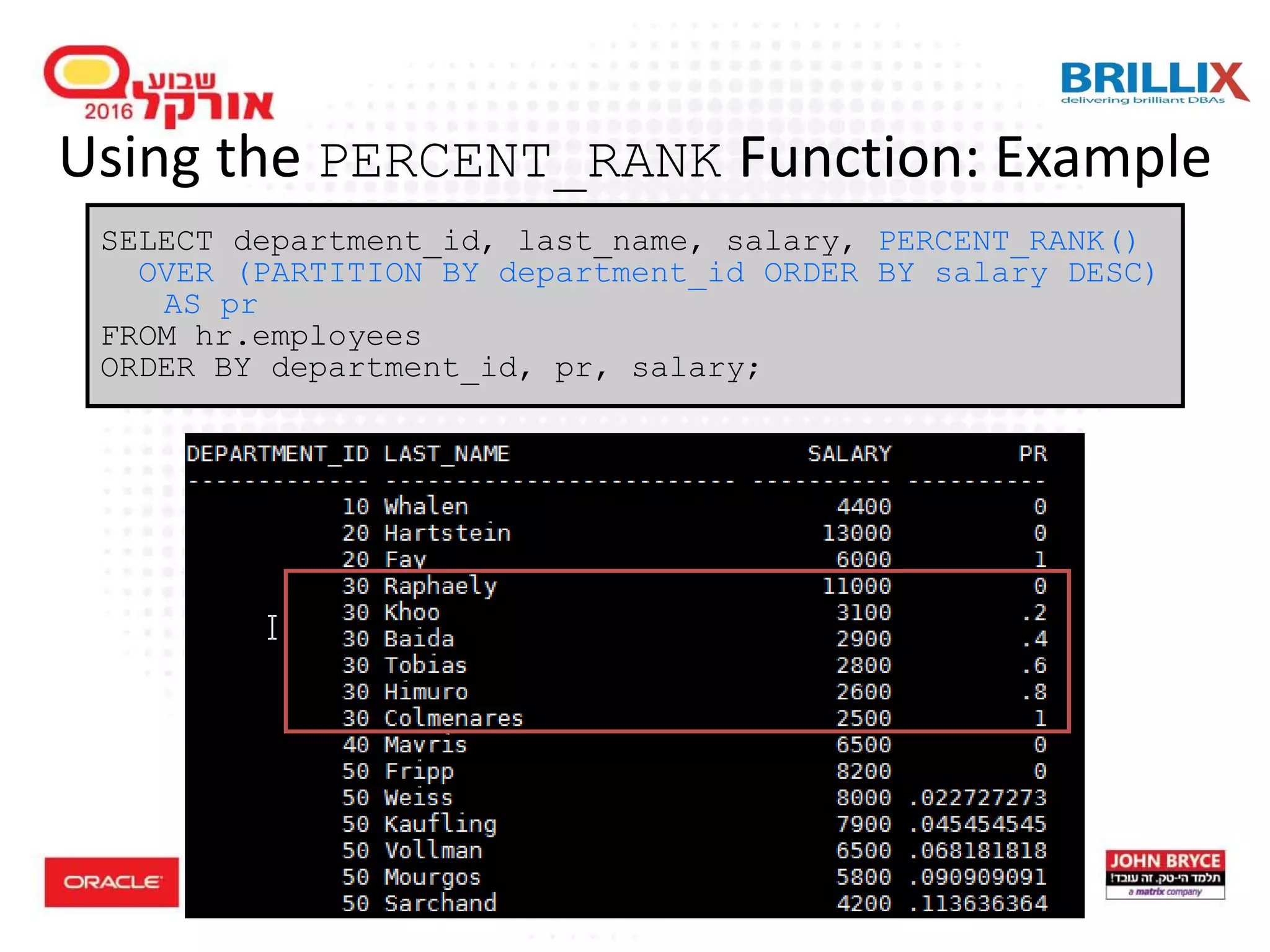
Introduction to analytic functions in SQL, focusing on rankings, partitions, and moving calculations.
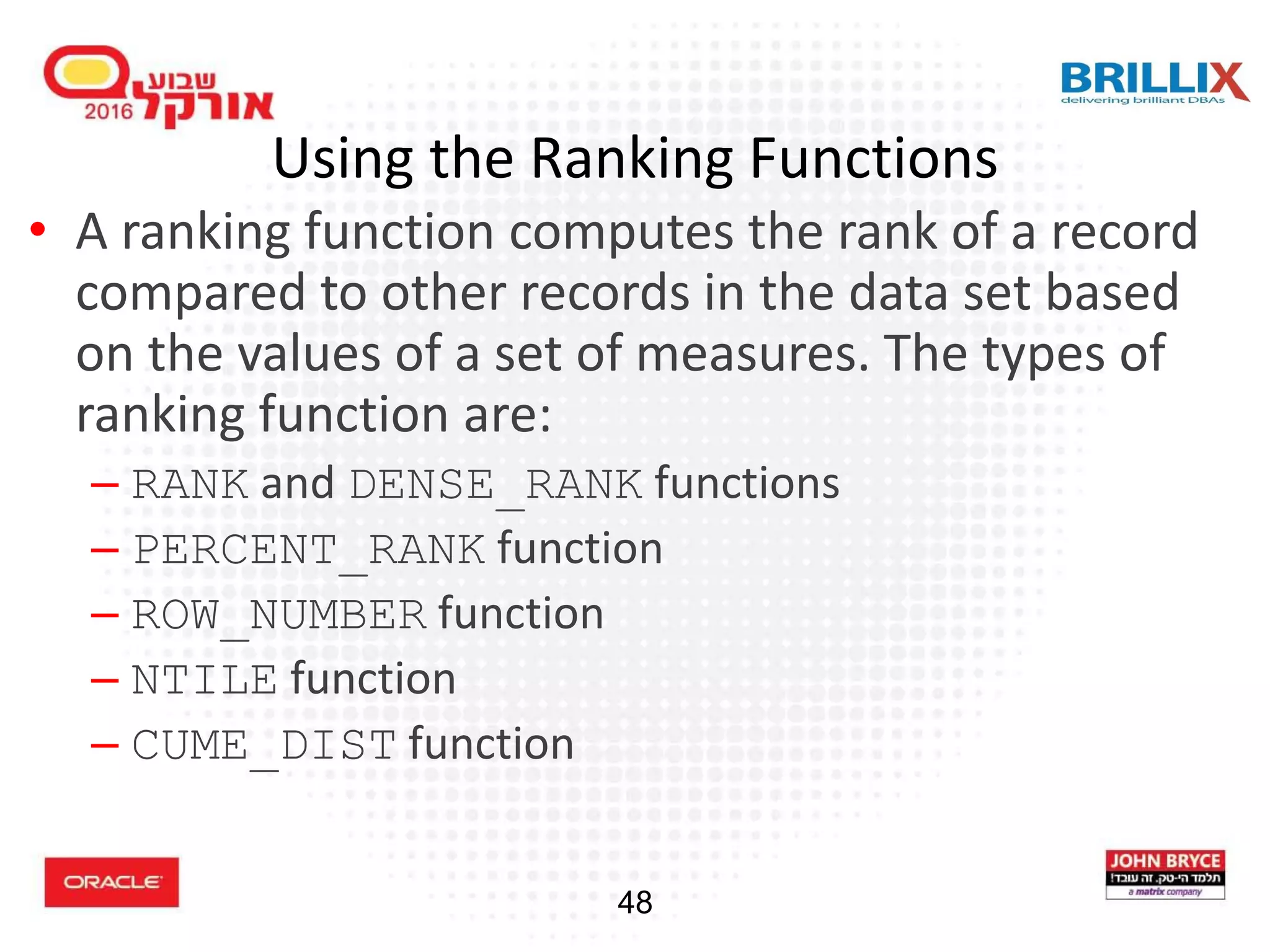
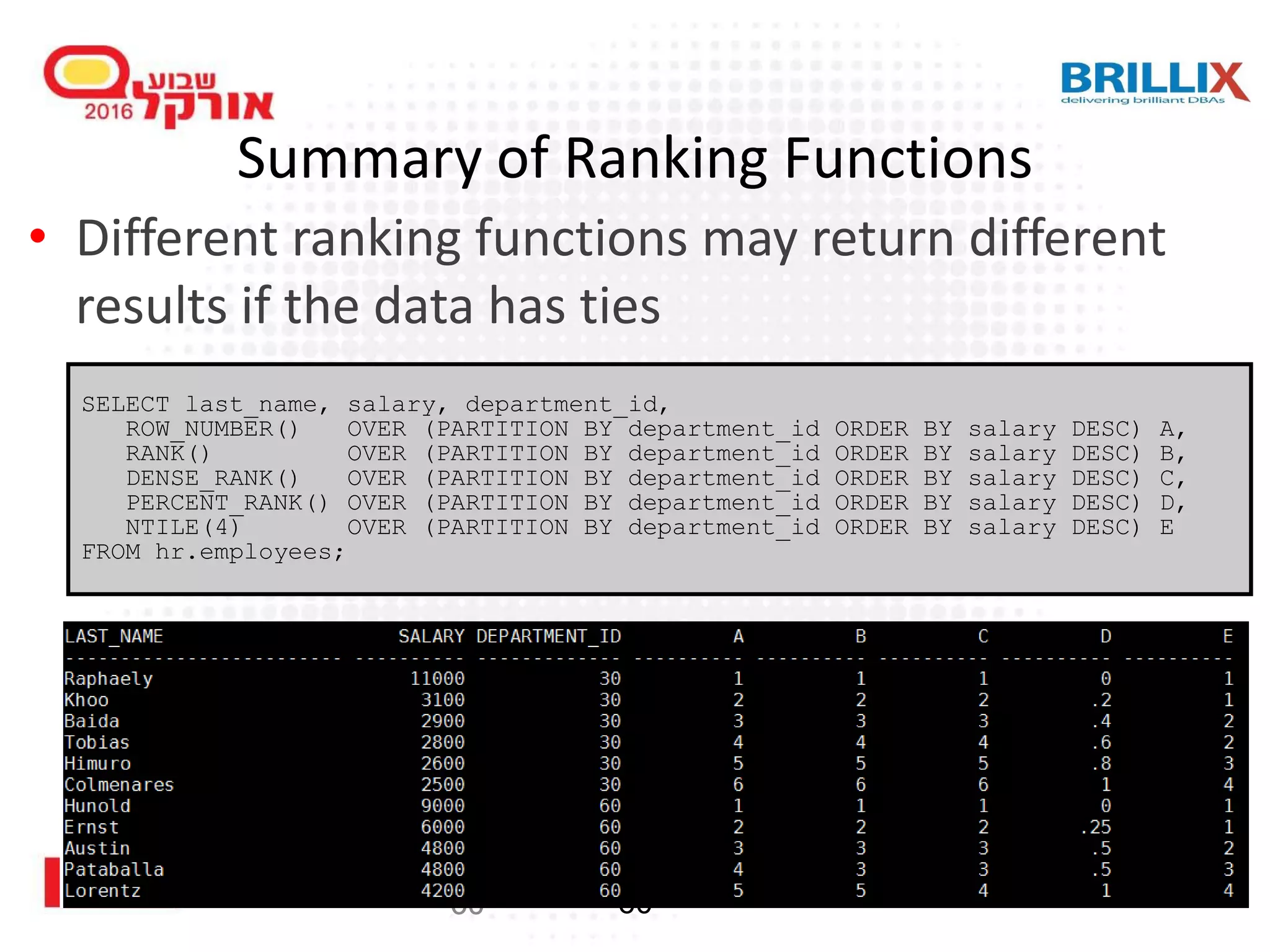
Understanding the advantages of using analytic functions to enhance query performance and data insight. Different ranking functions such as RANK, DENSE_RANK, and their usage in SQL queries with examples.
Usage of LAG and LEAD analytic functions for accessing previous or following rows in datasets.
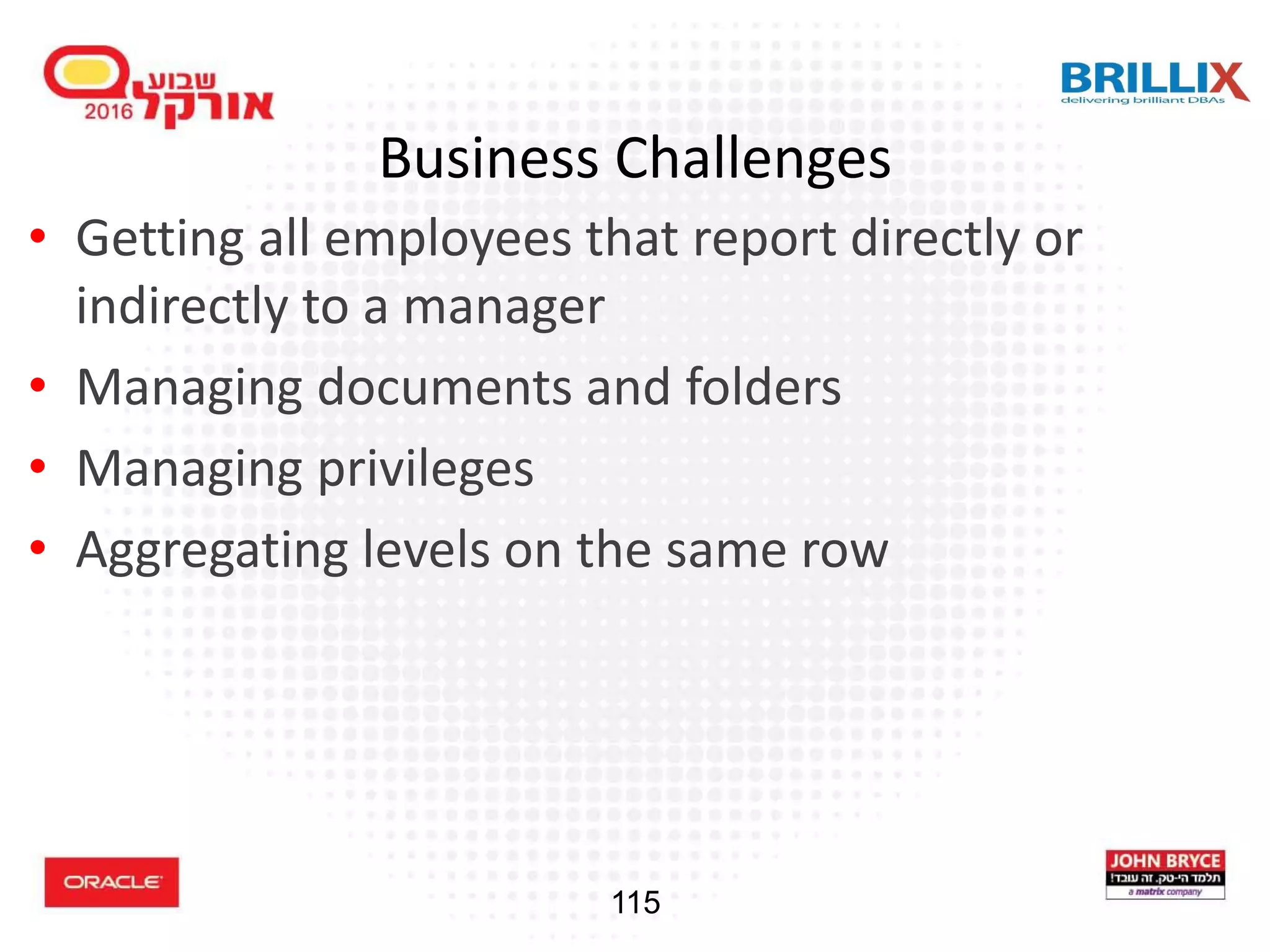
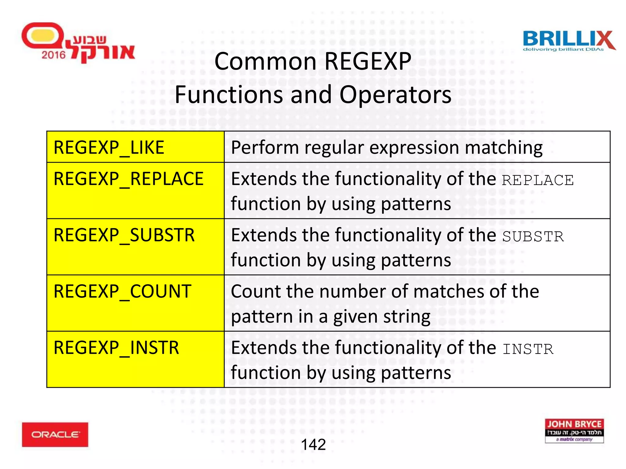
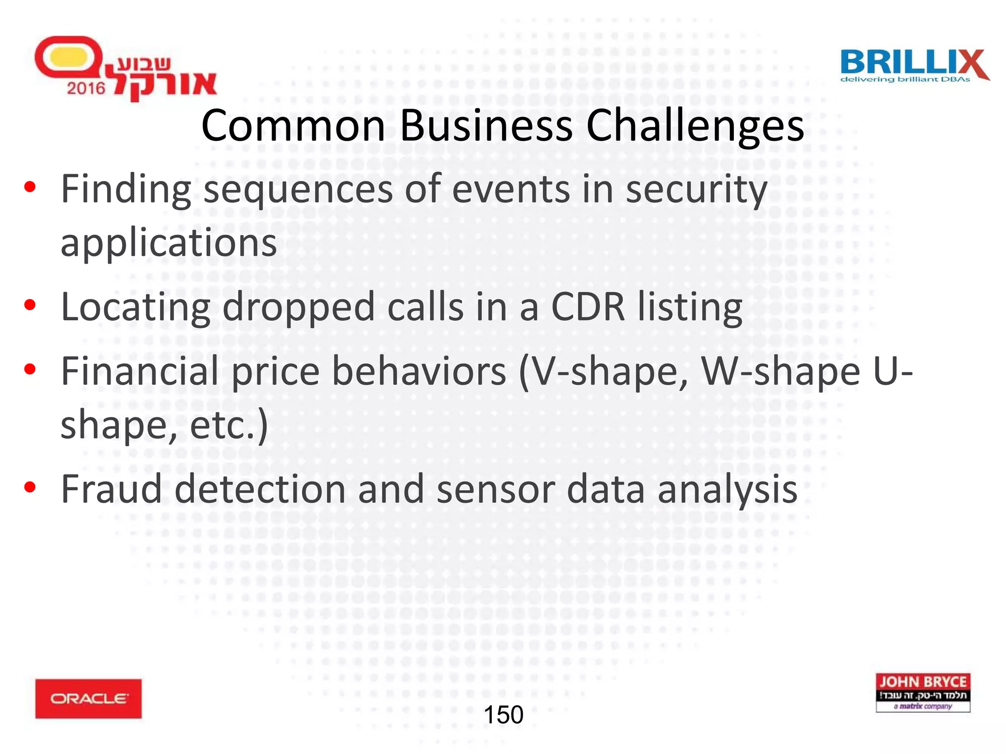
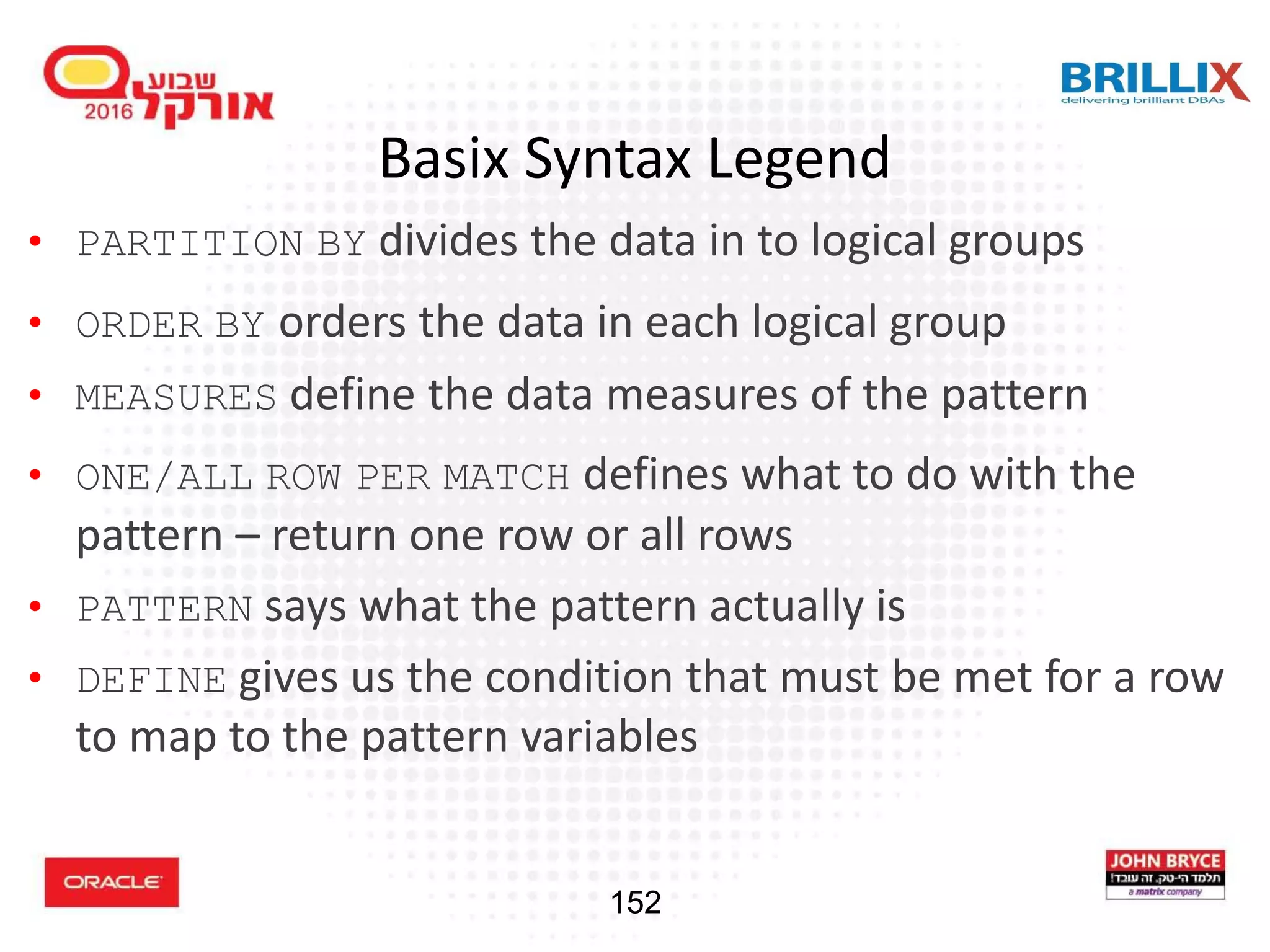
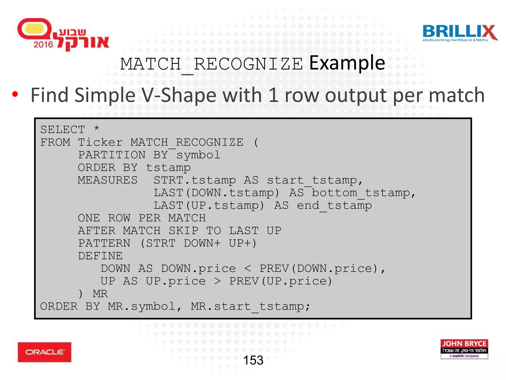
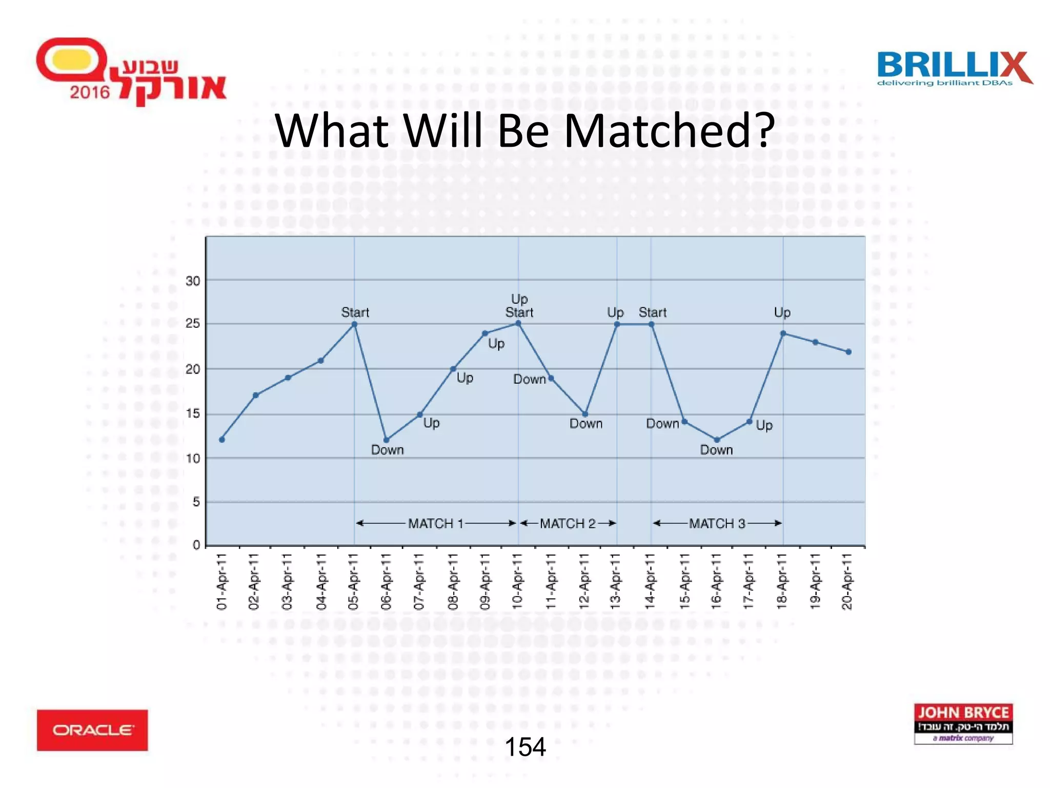
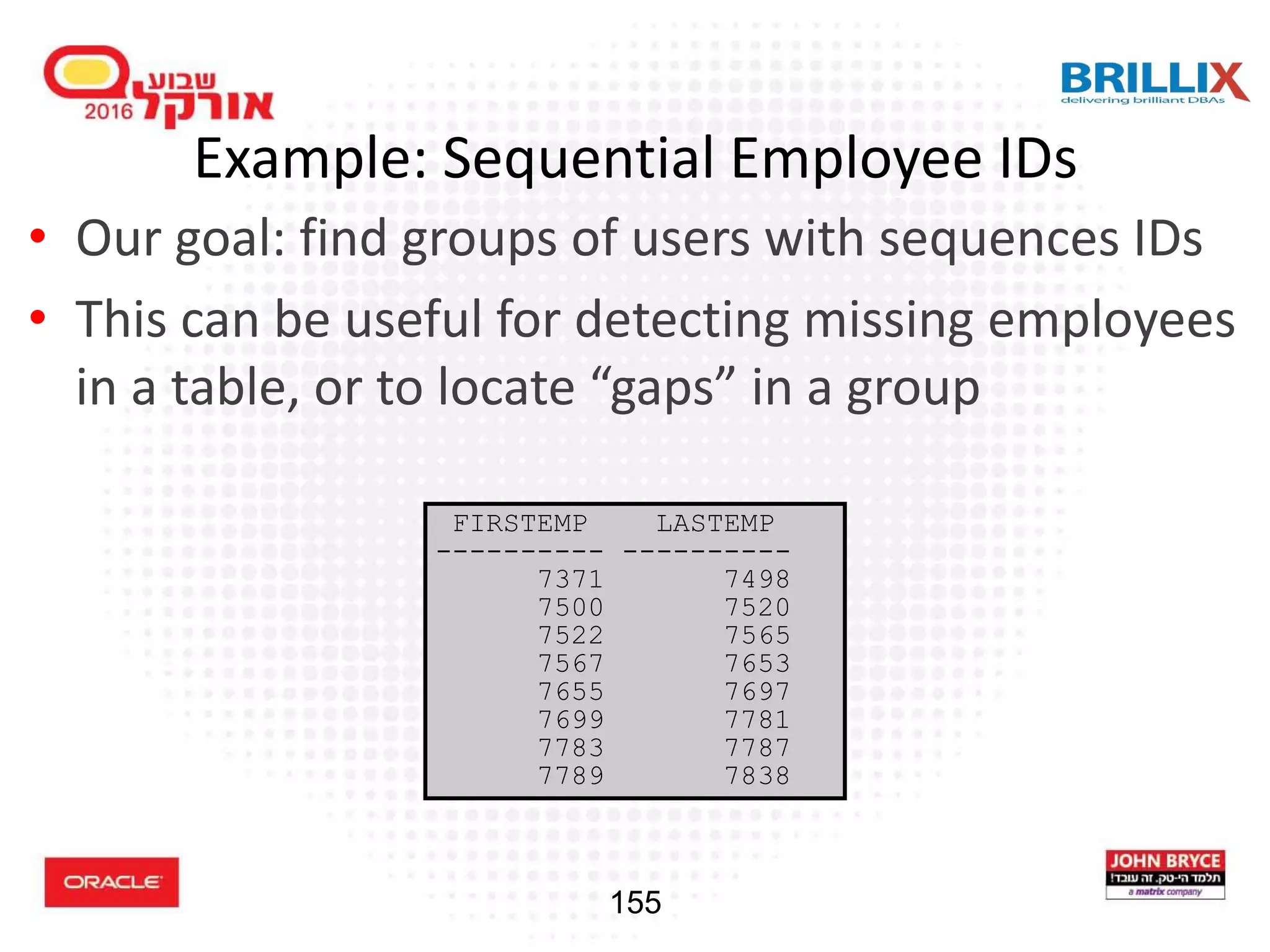
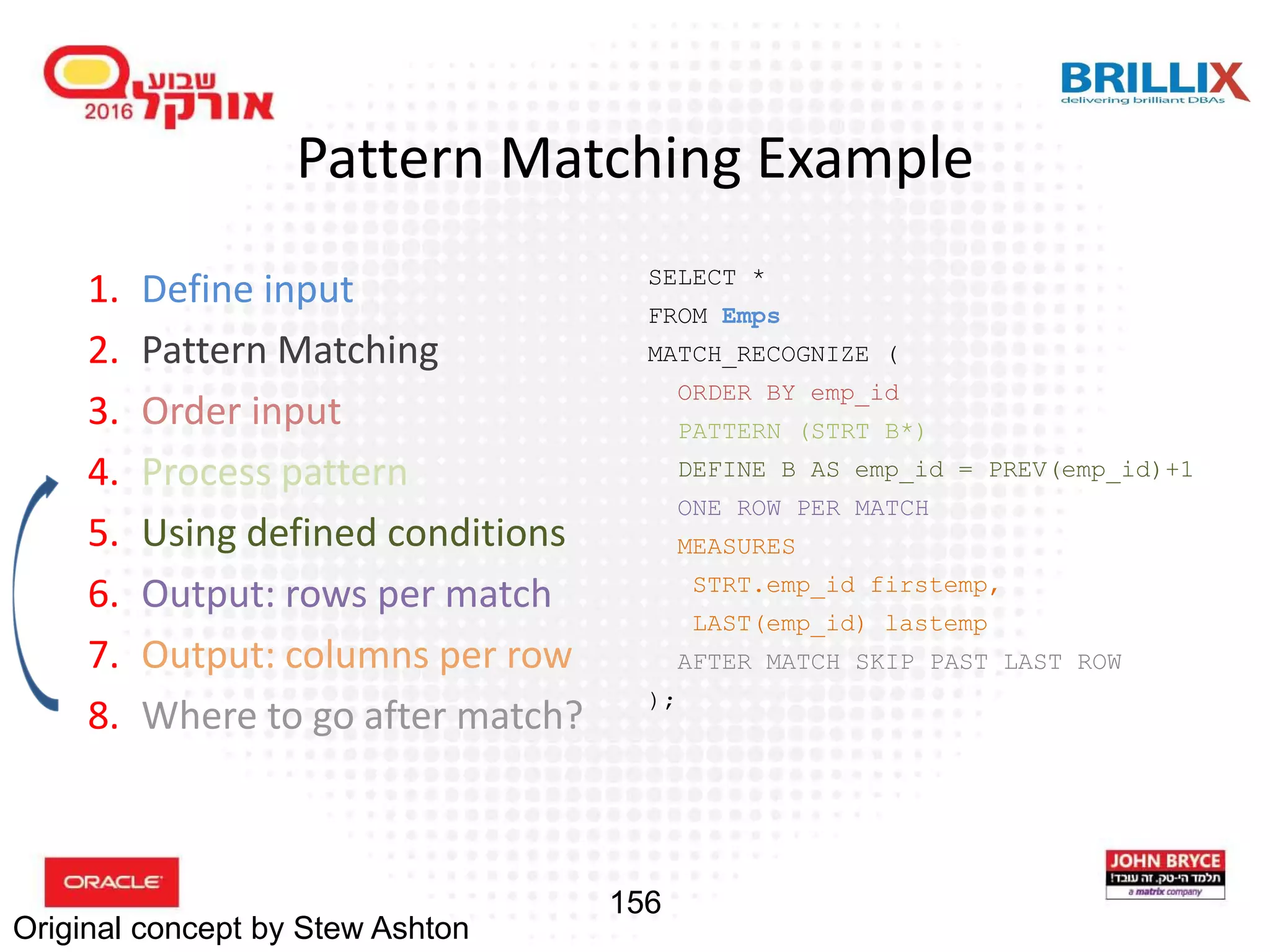
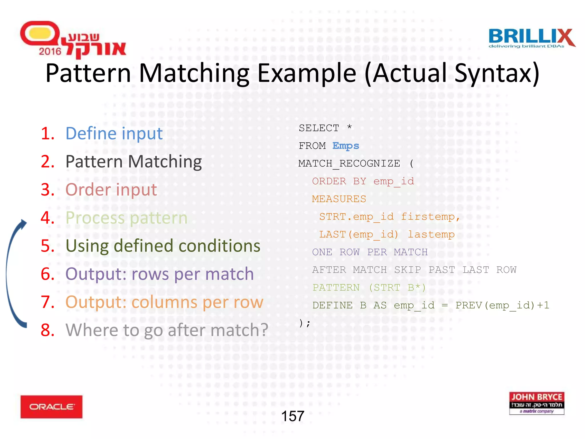
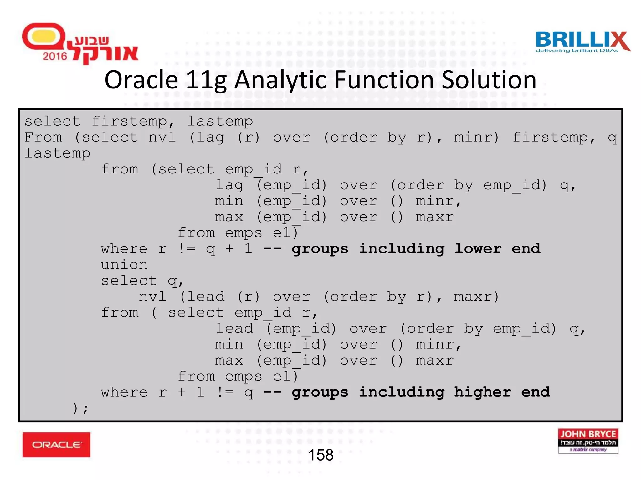
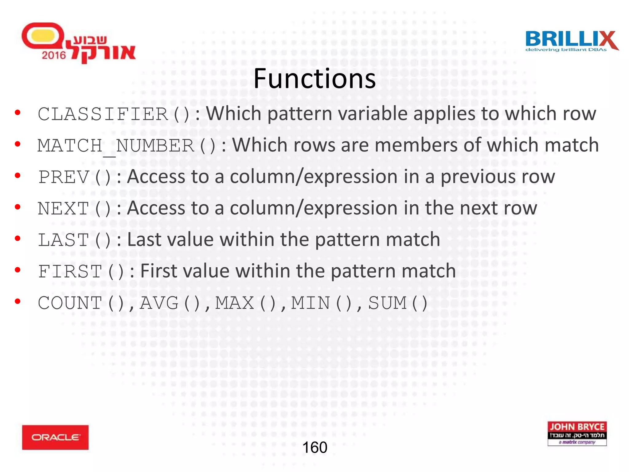
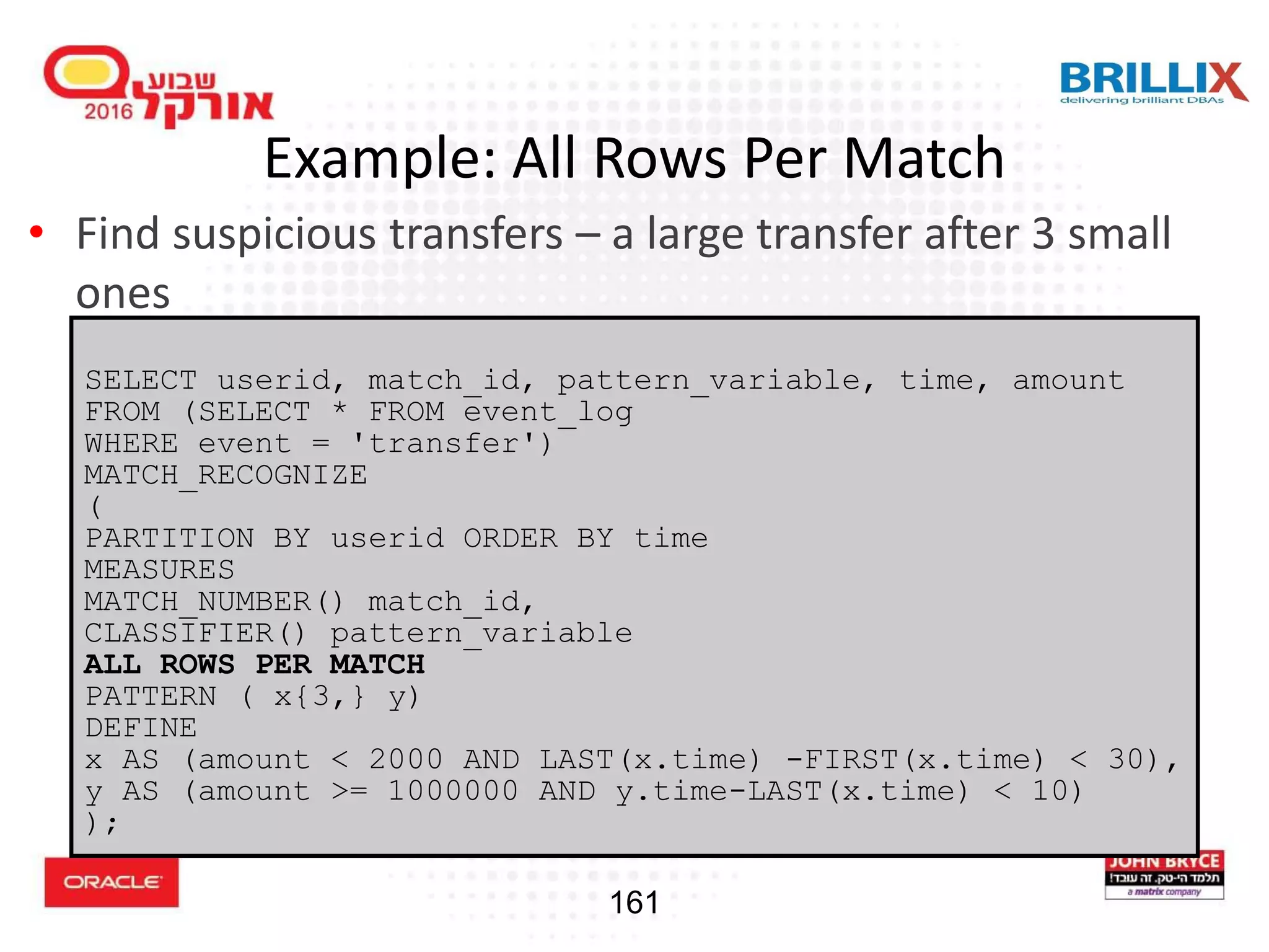
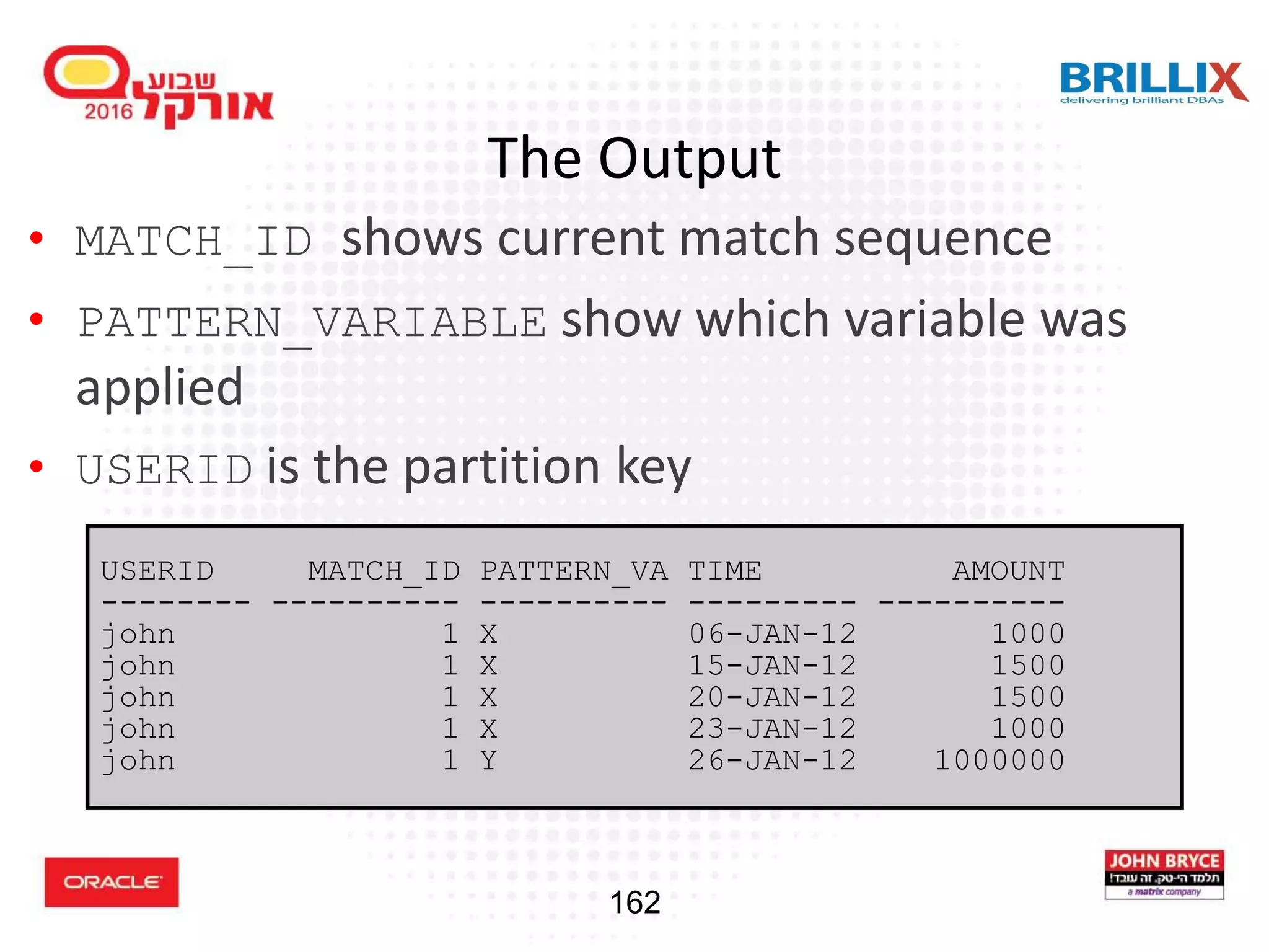
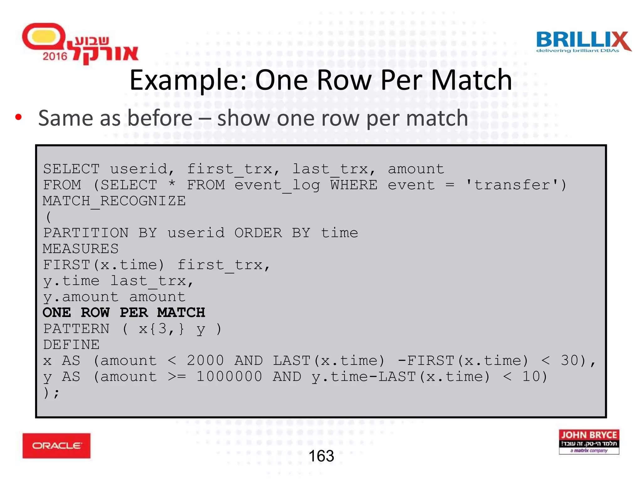
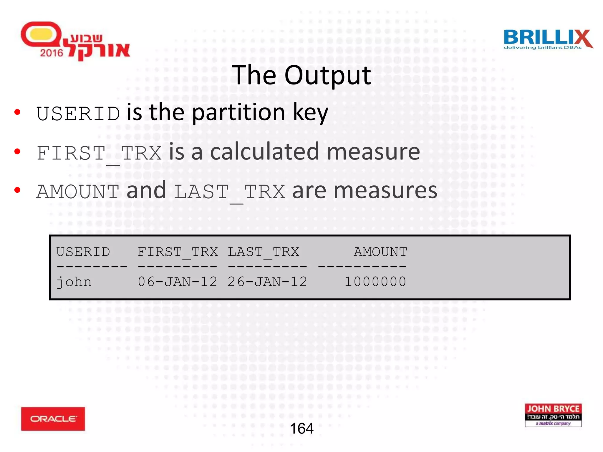
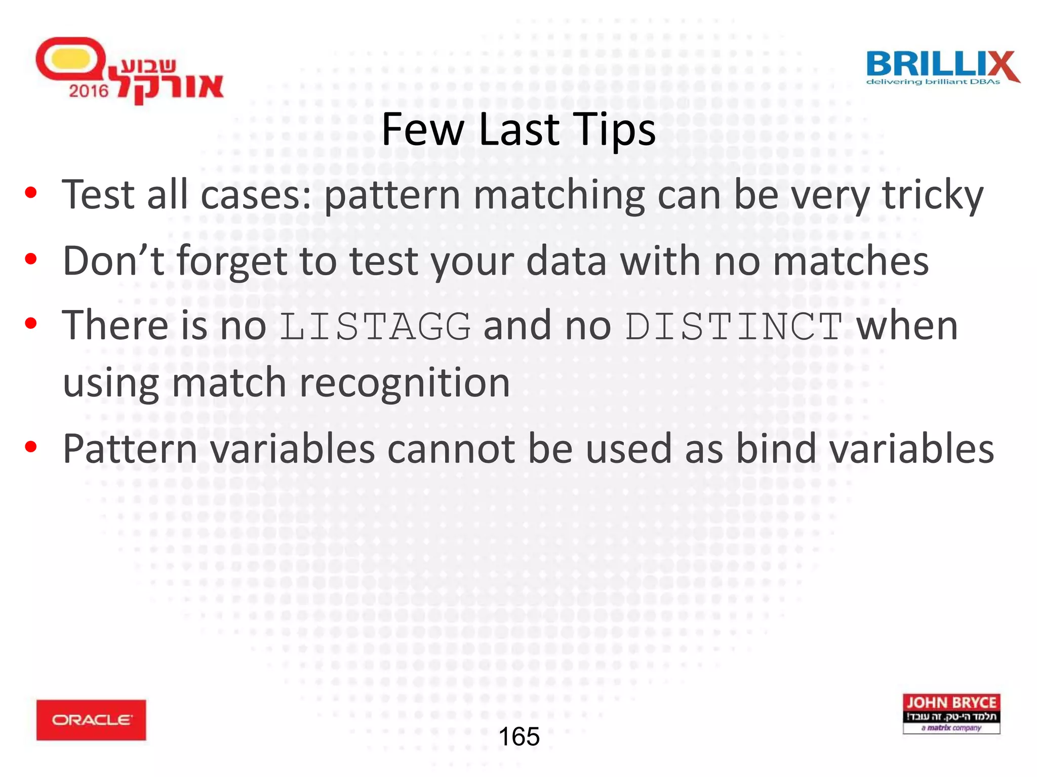
Introduction to pattern matching in SQL, along with common business challenges and effective solutions.
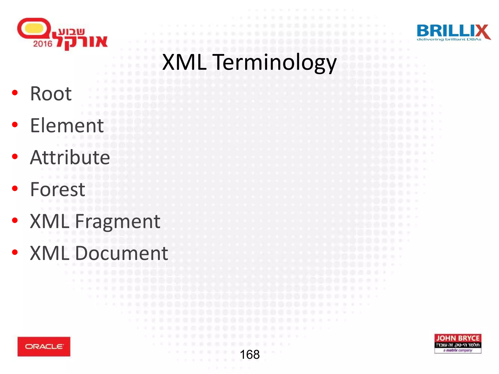
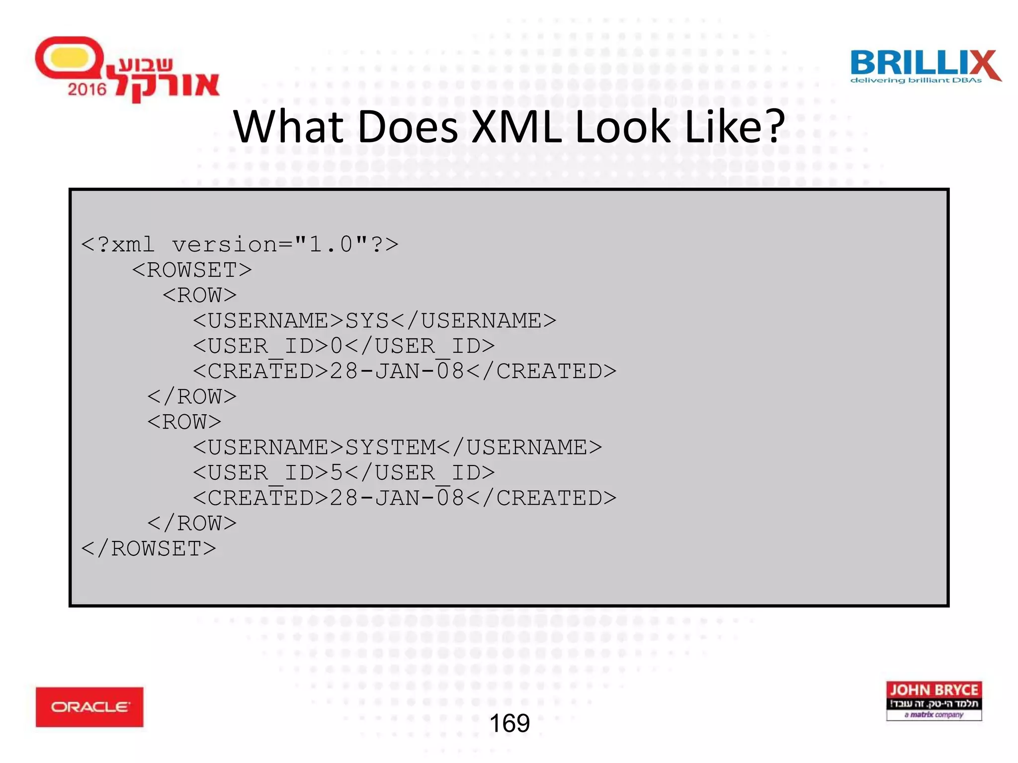
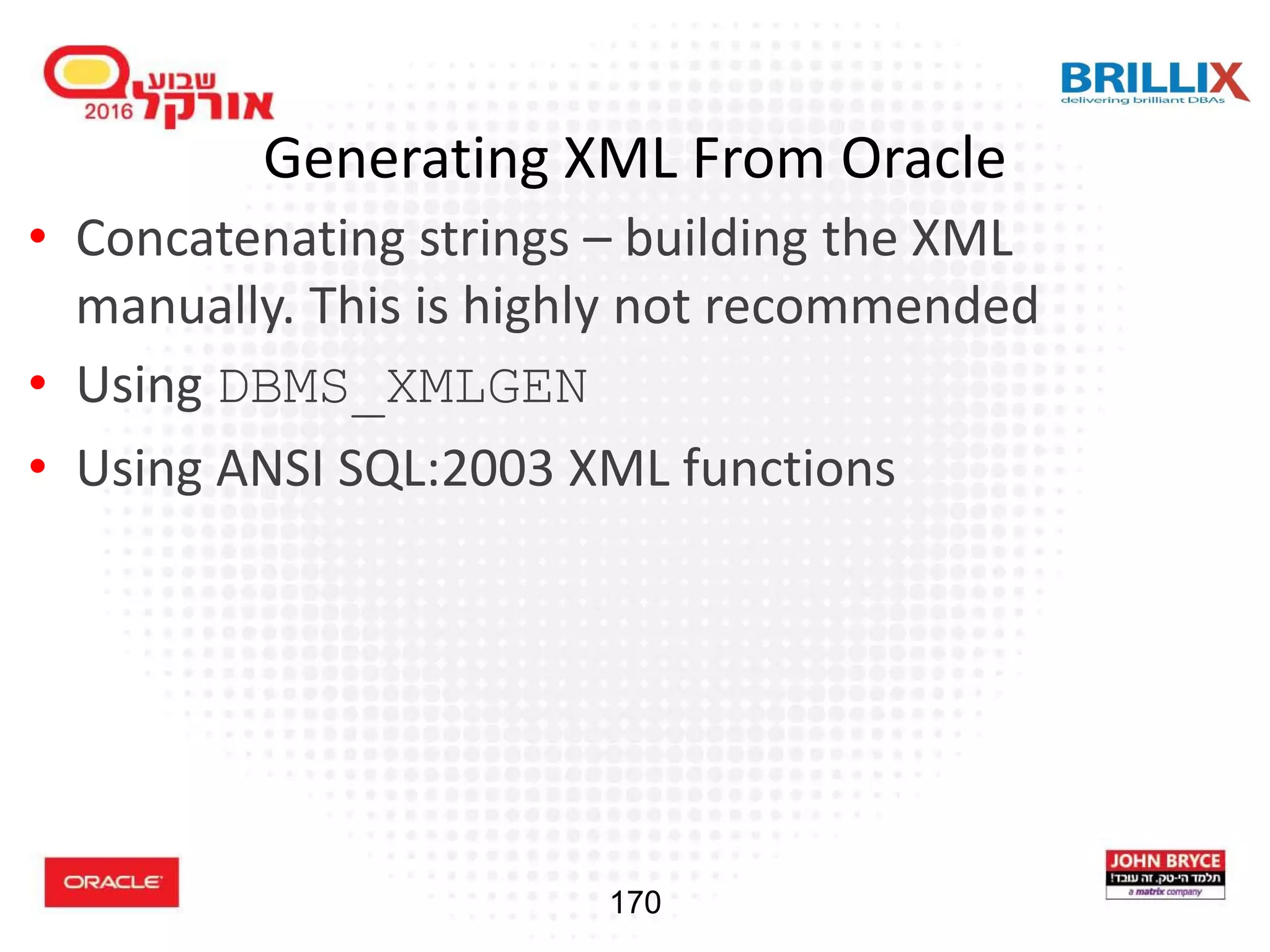
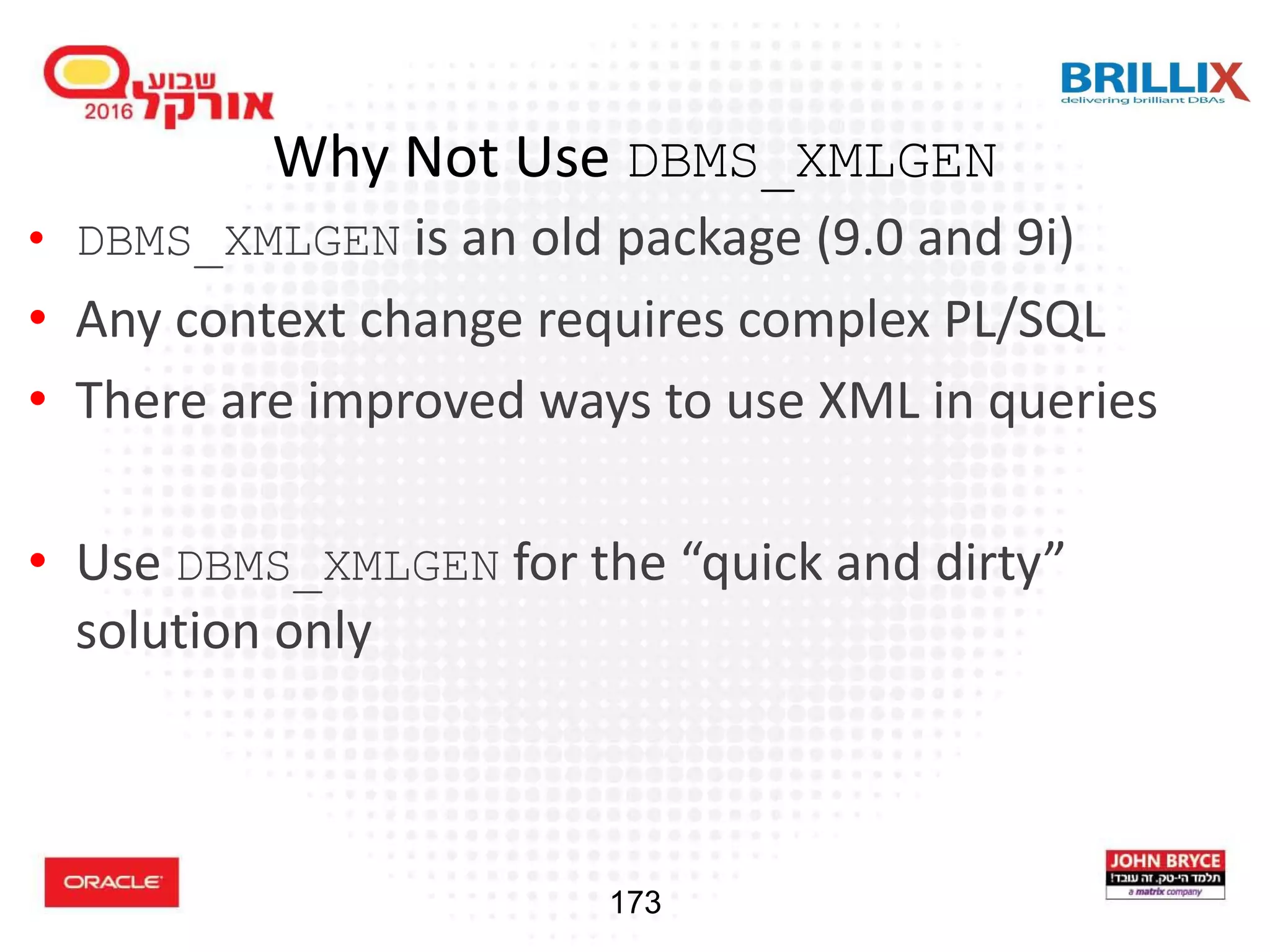
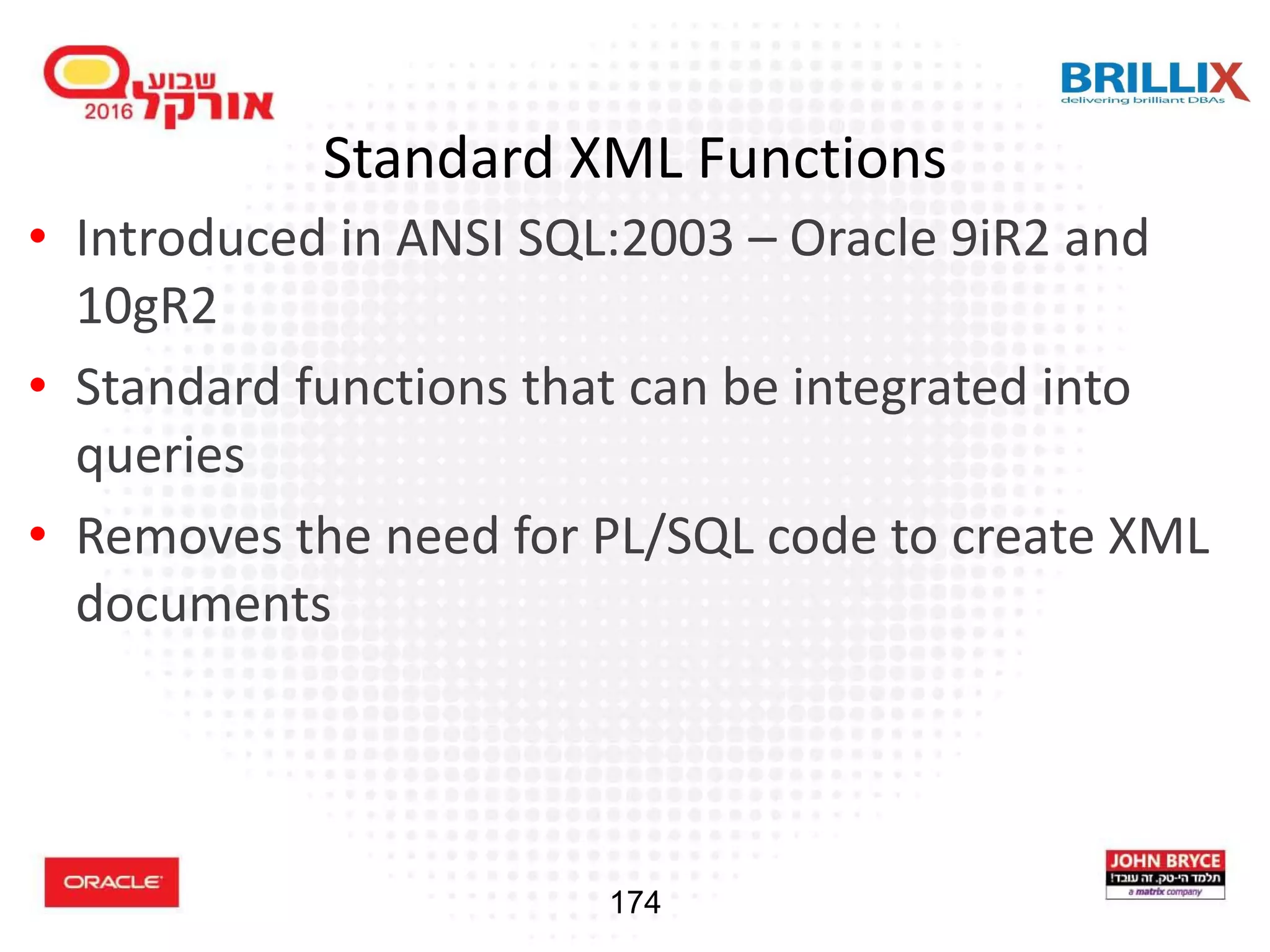
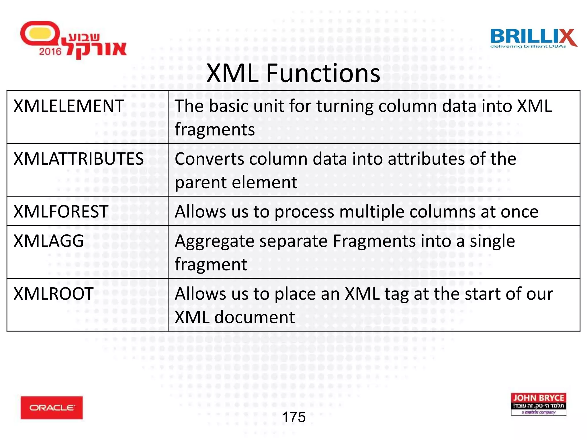
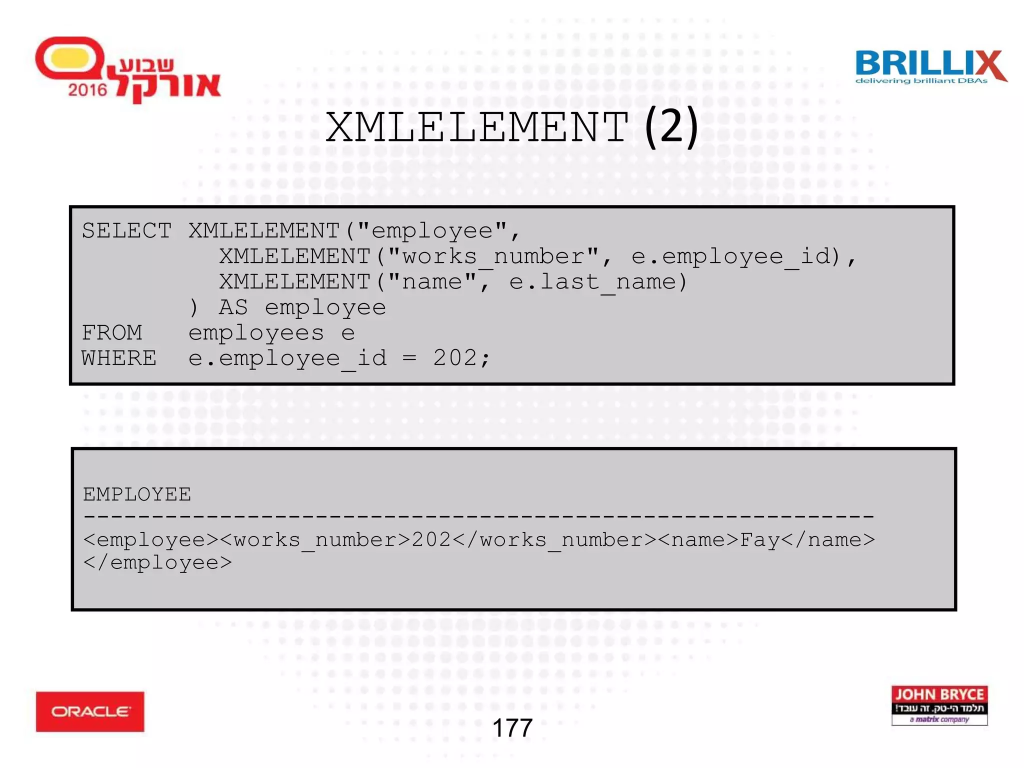
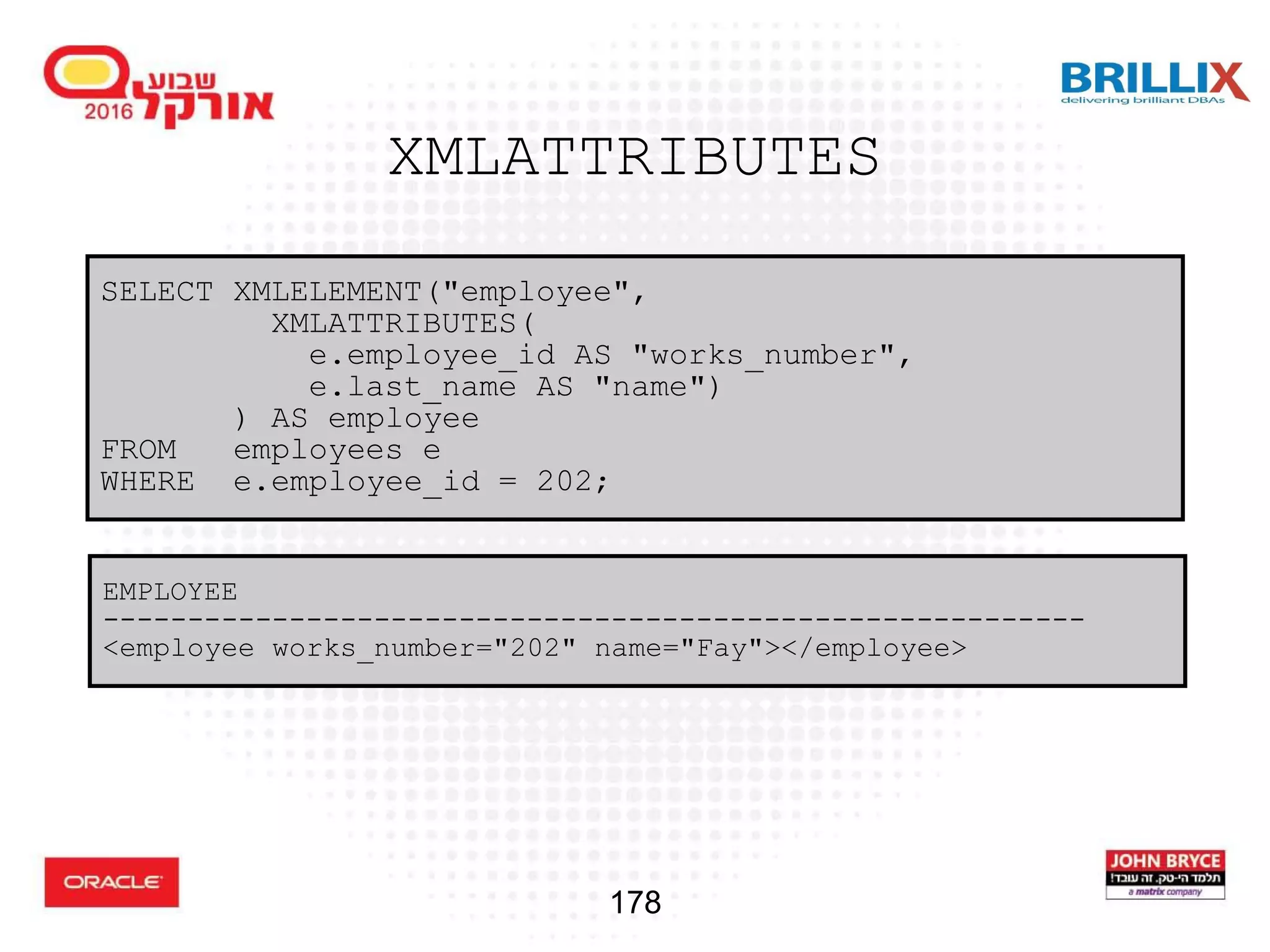
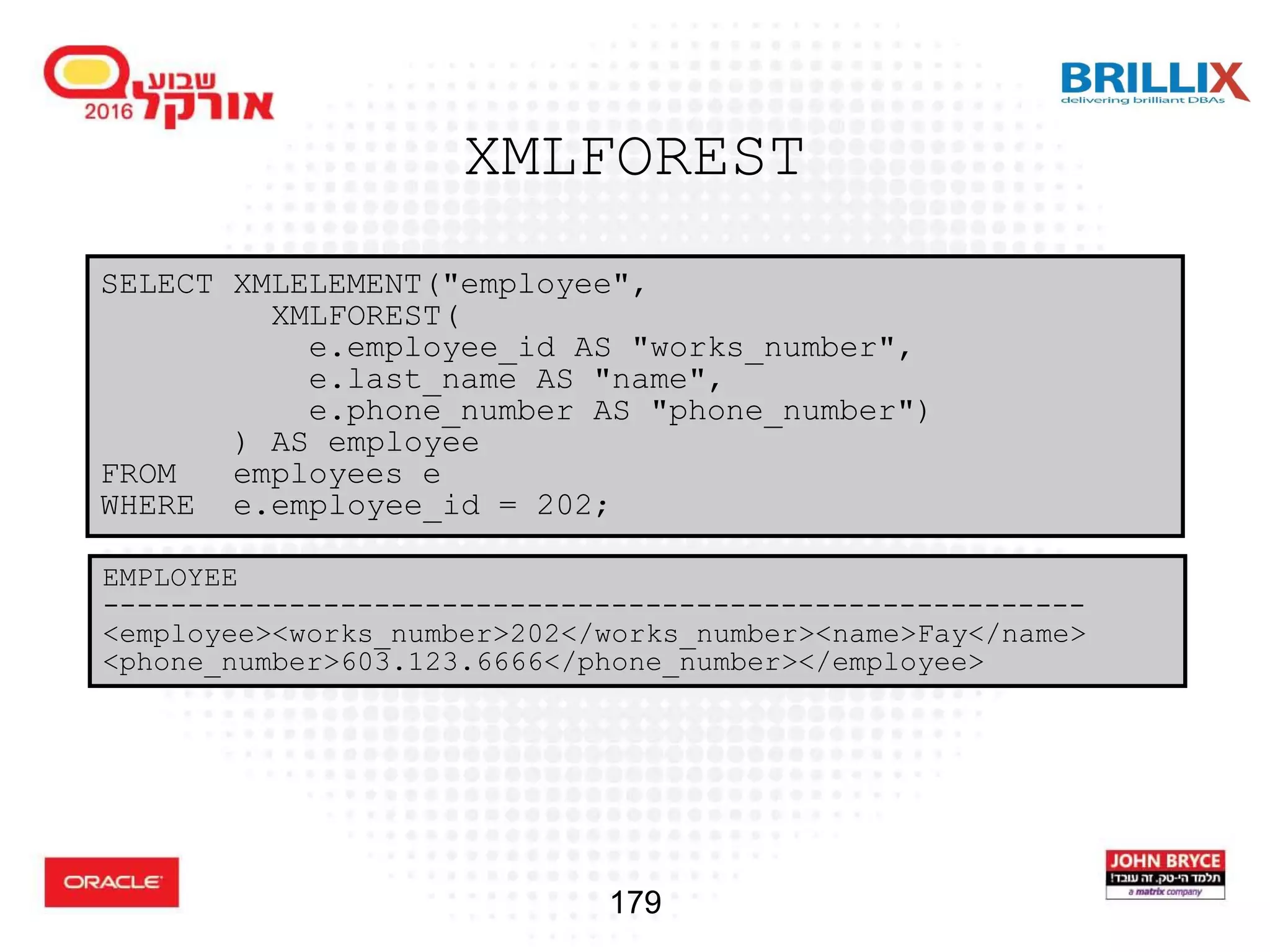
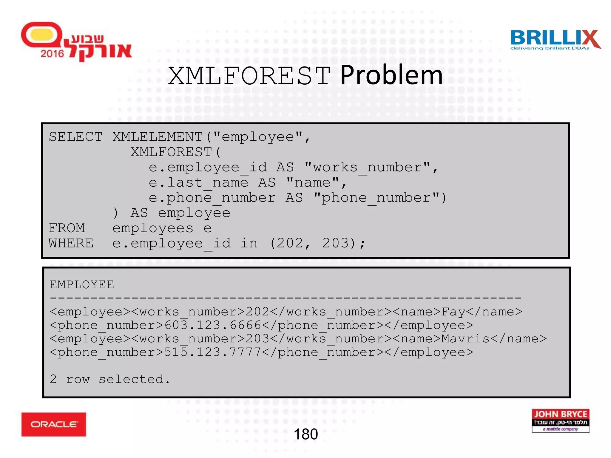
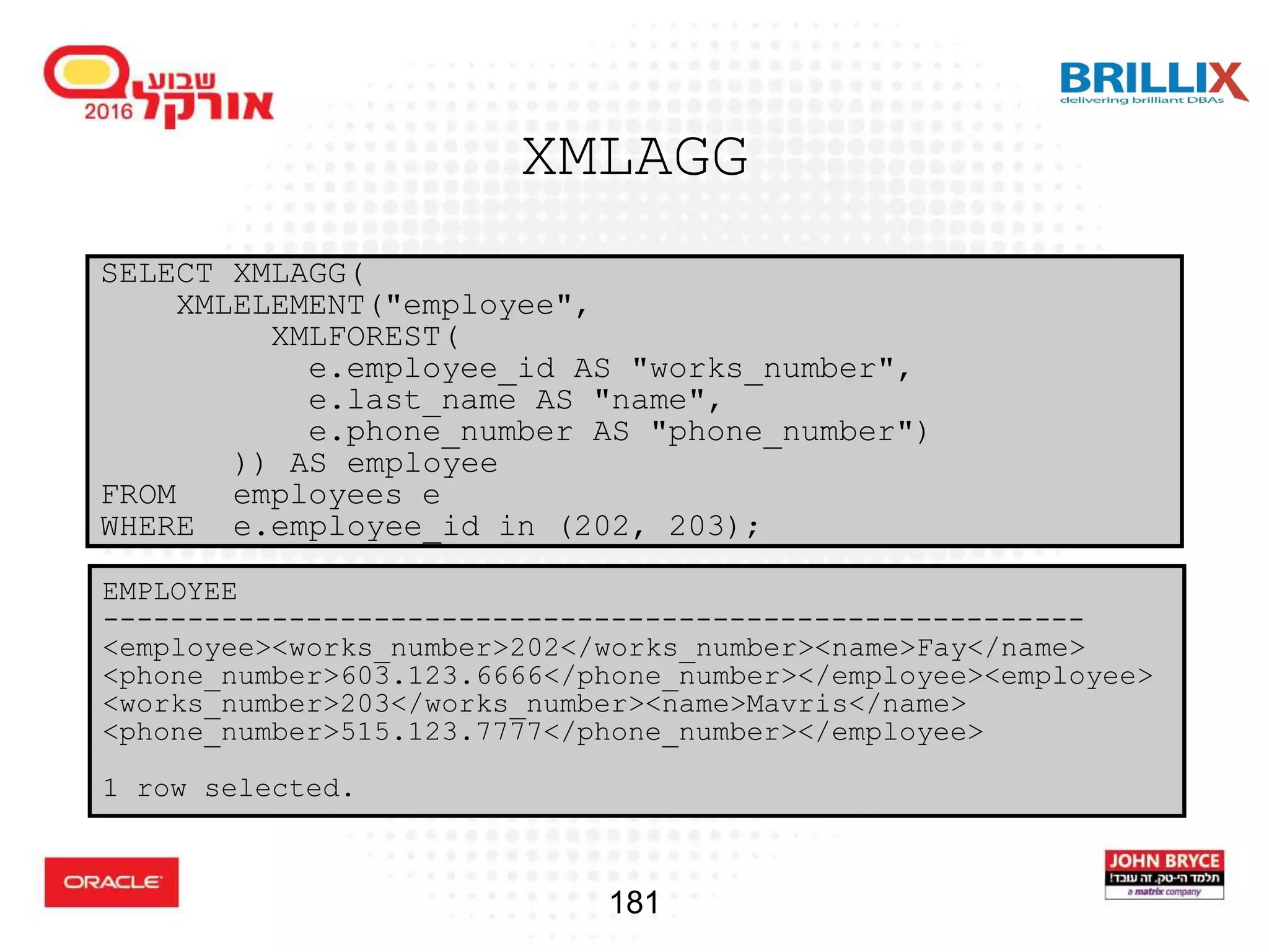
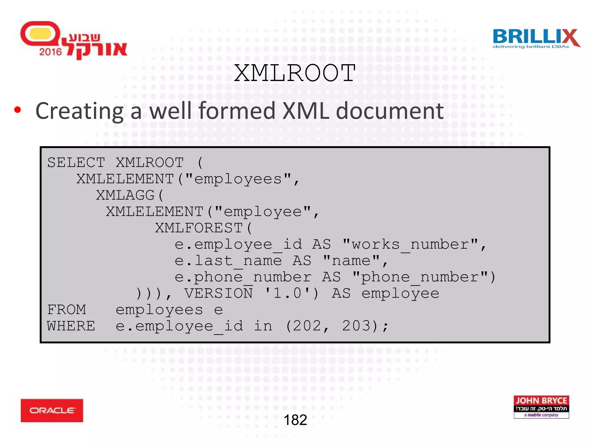
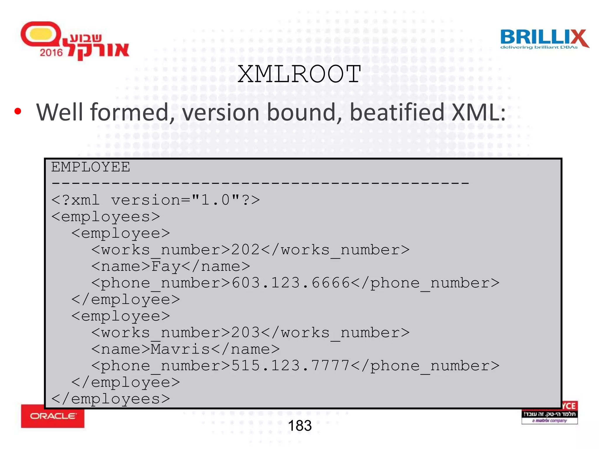
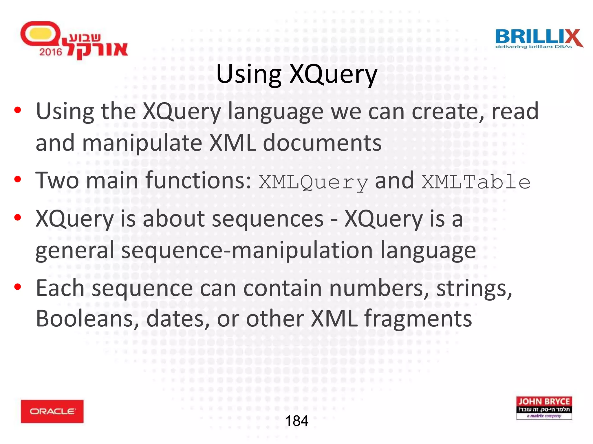
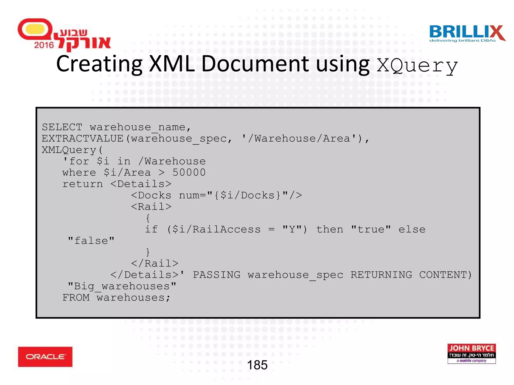
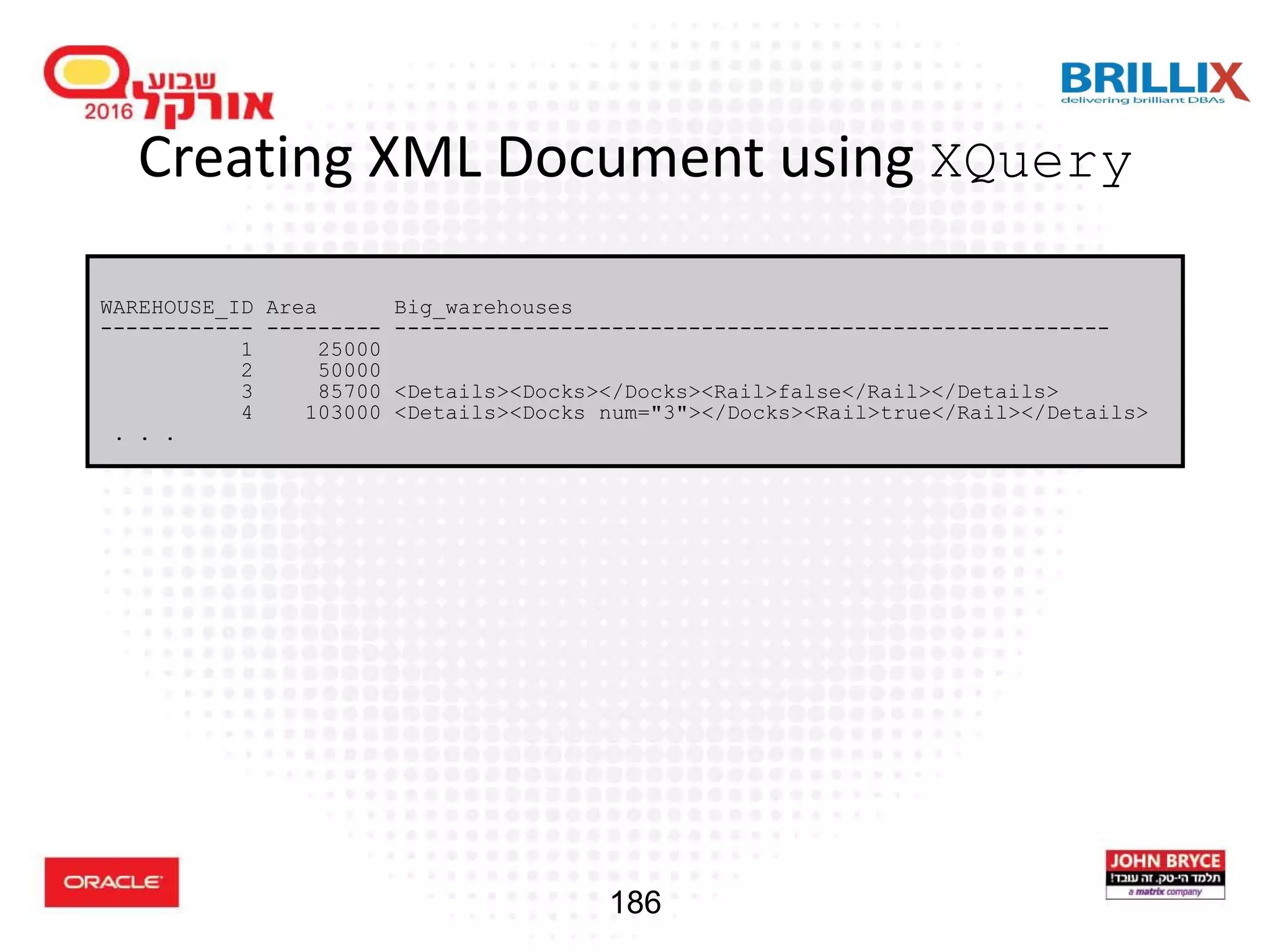
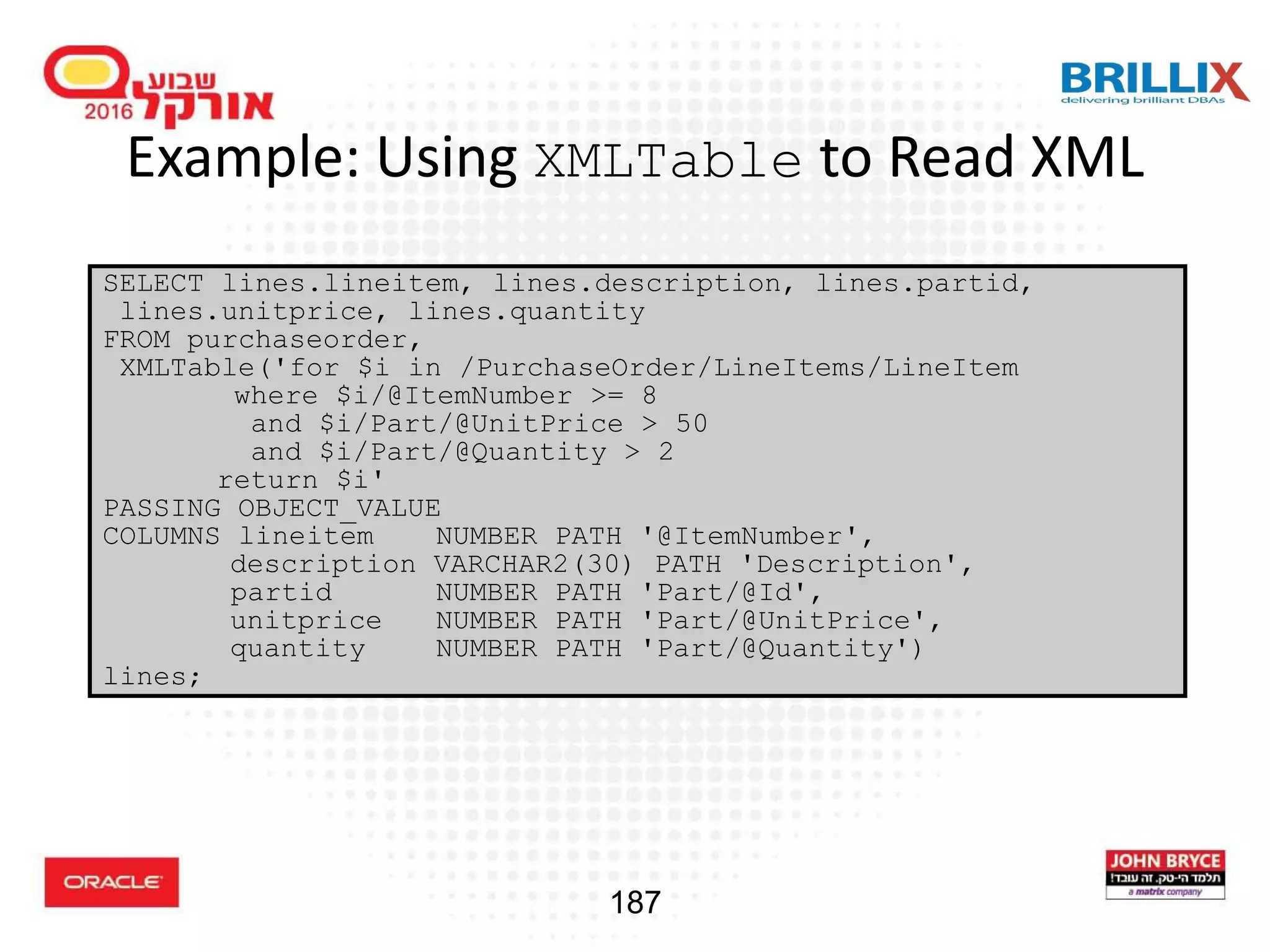
Overview of XML capabilities in Oracle SQL, including generation, structure, and data manipulation.
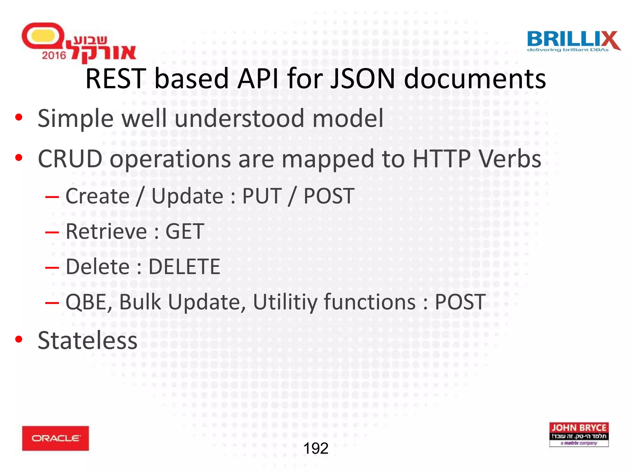
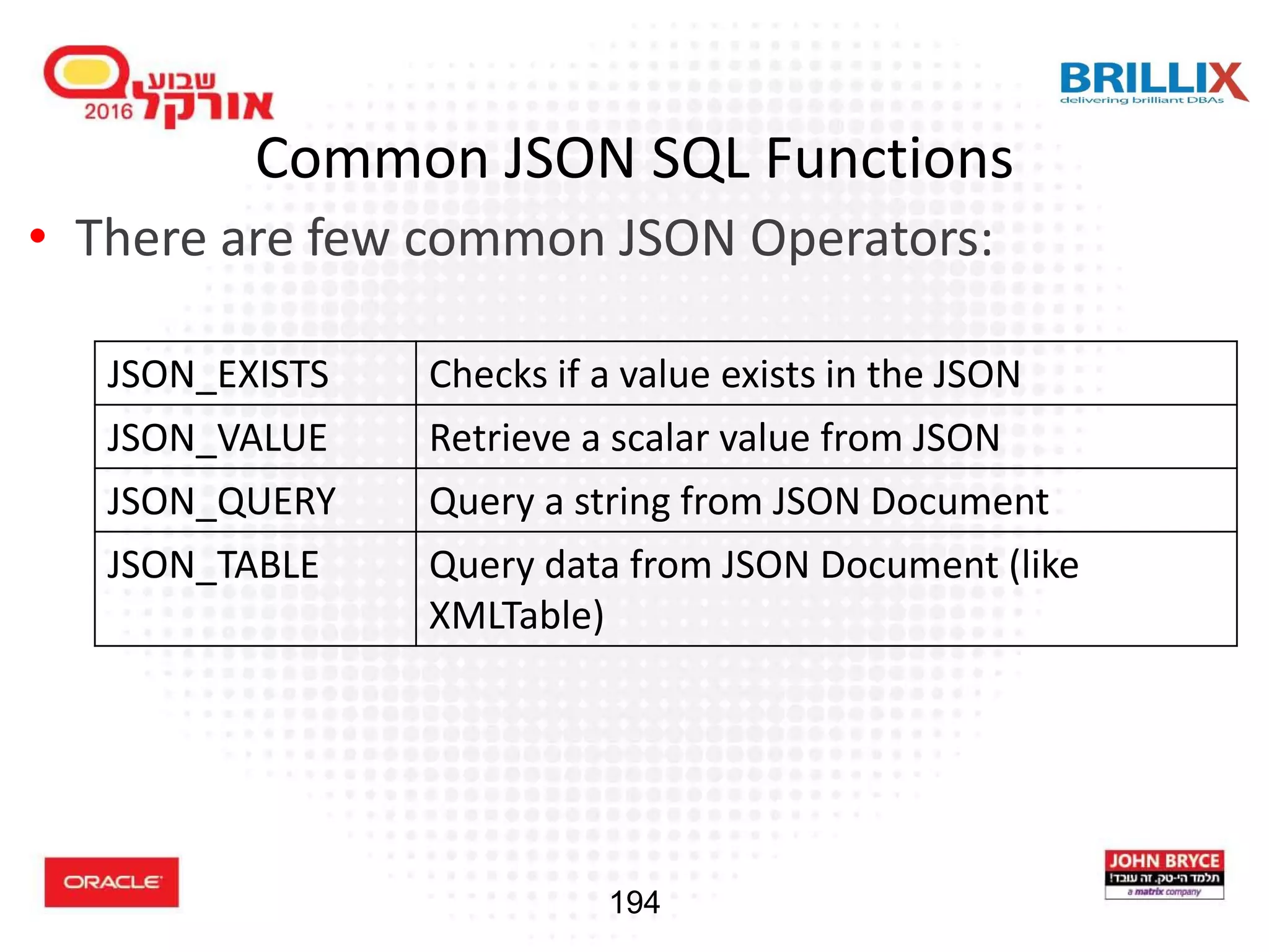
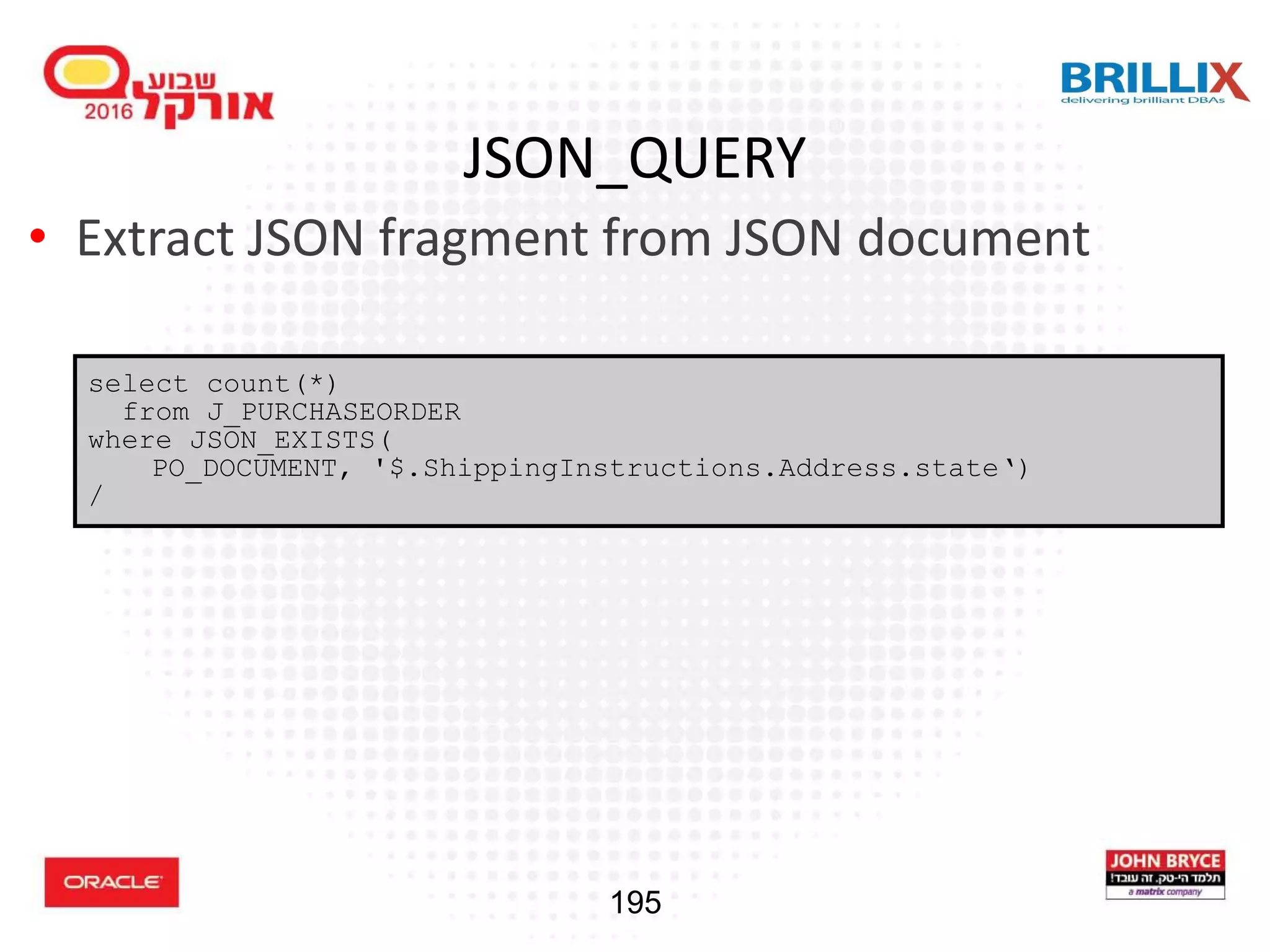
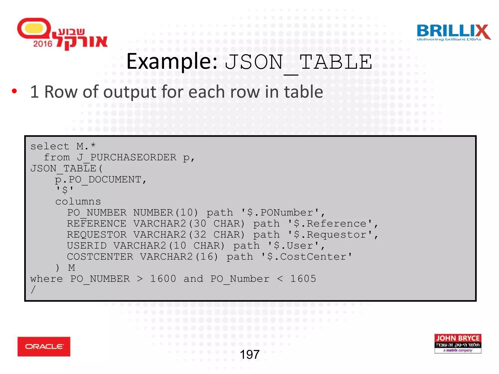
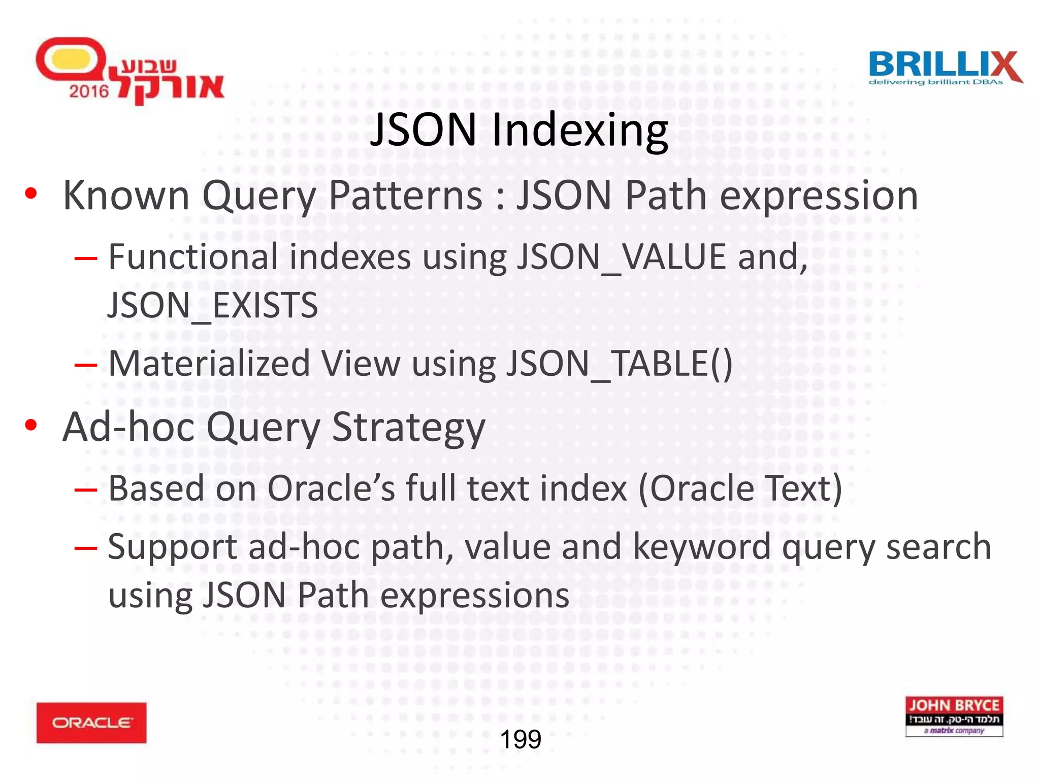
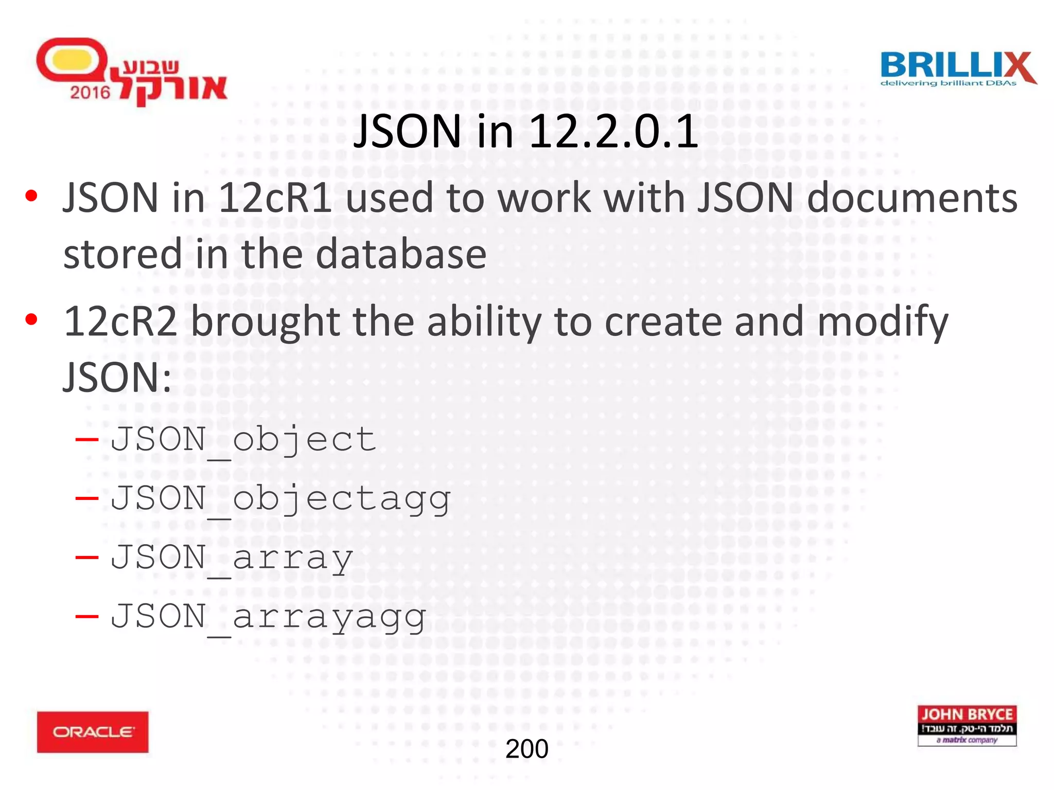
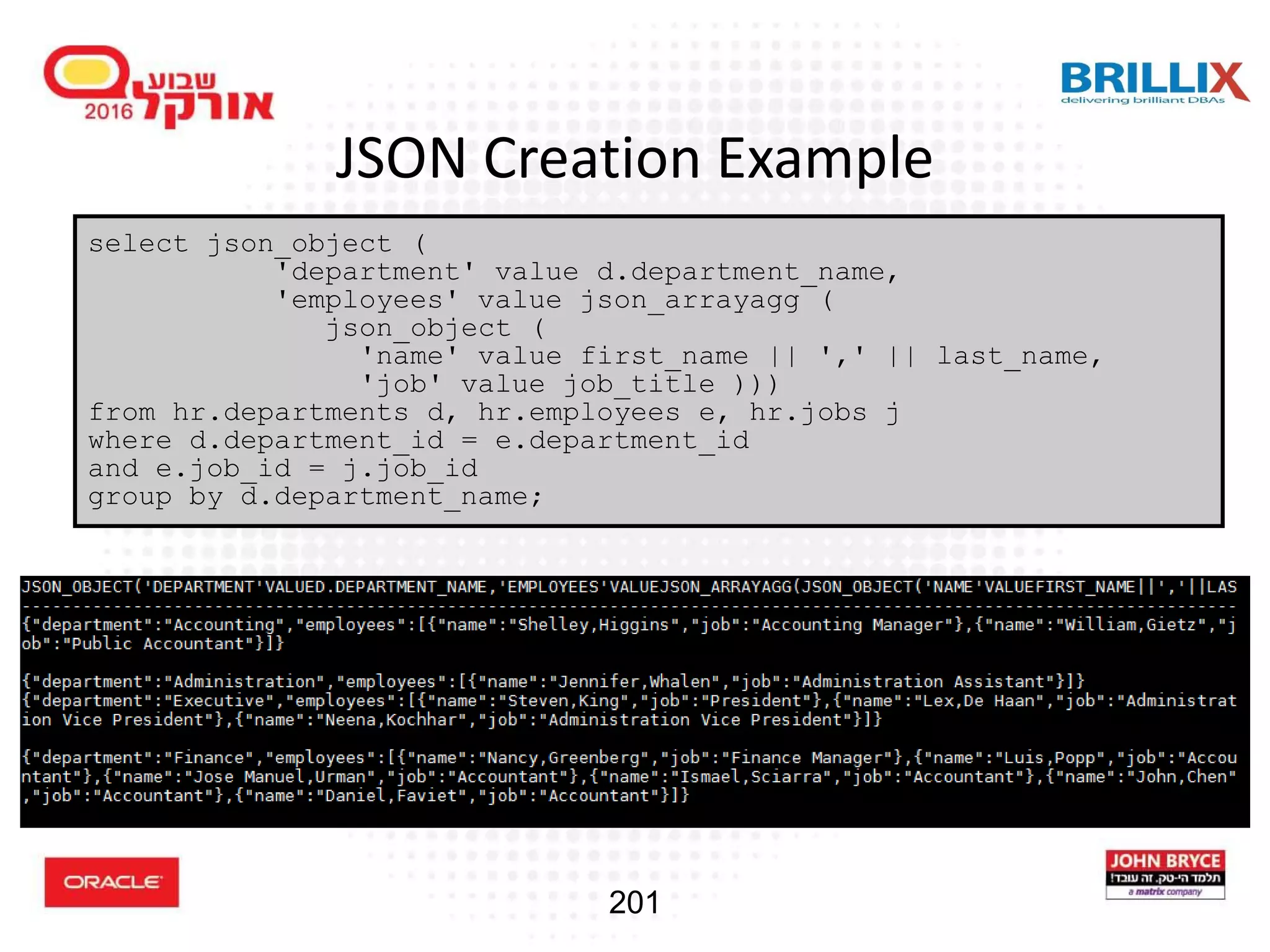
Discussion on JSON data handling, including benefits, SQL functions, and examples within Oracle 12c.
Introduction to new features in Oracle 12c, including improved data handling and performance enhancements.
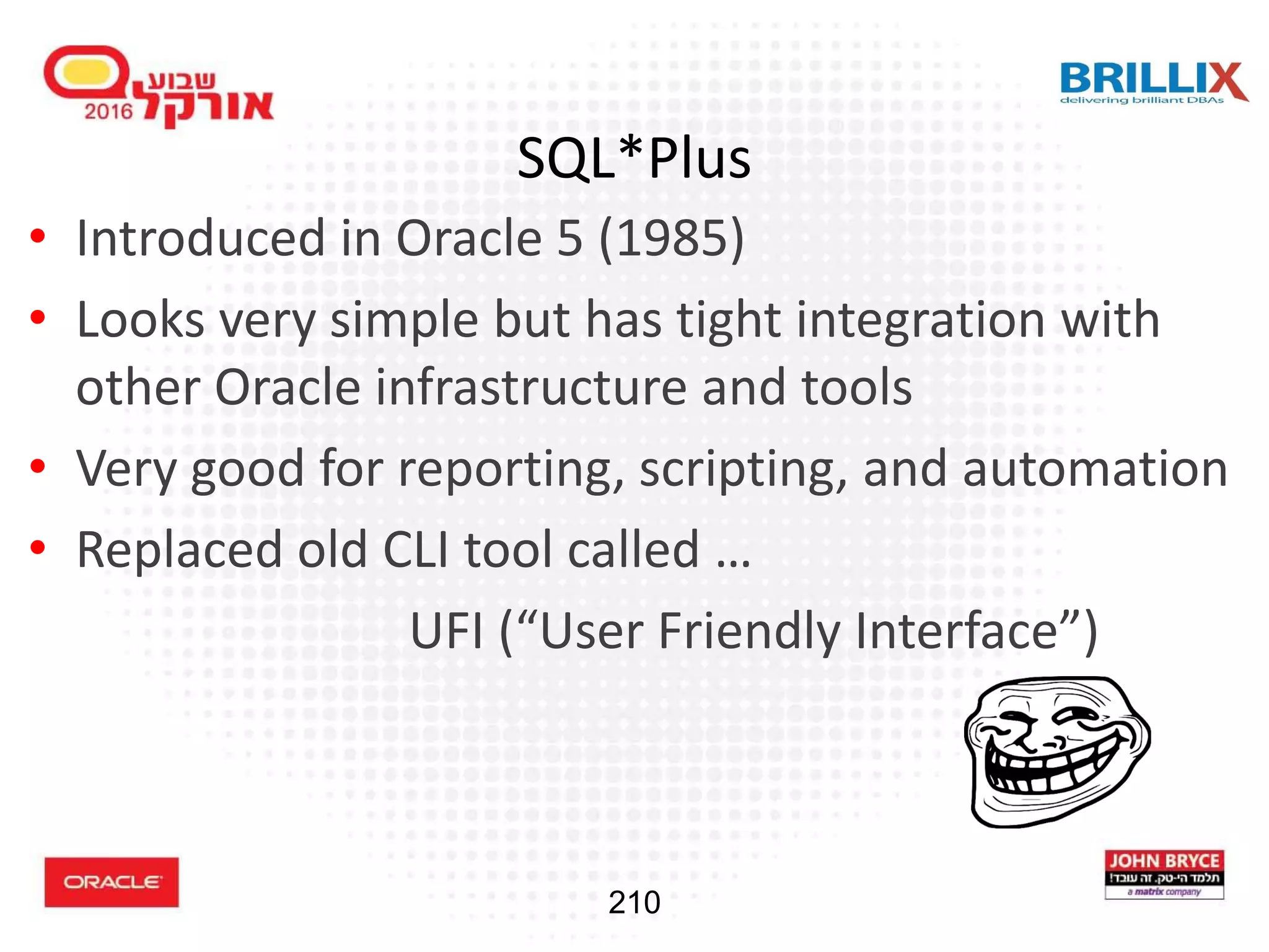
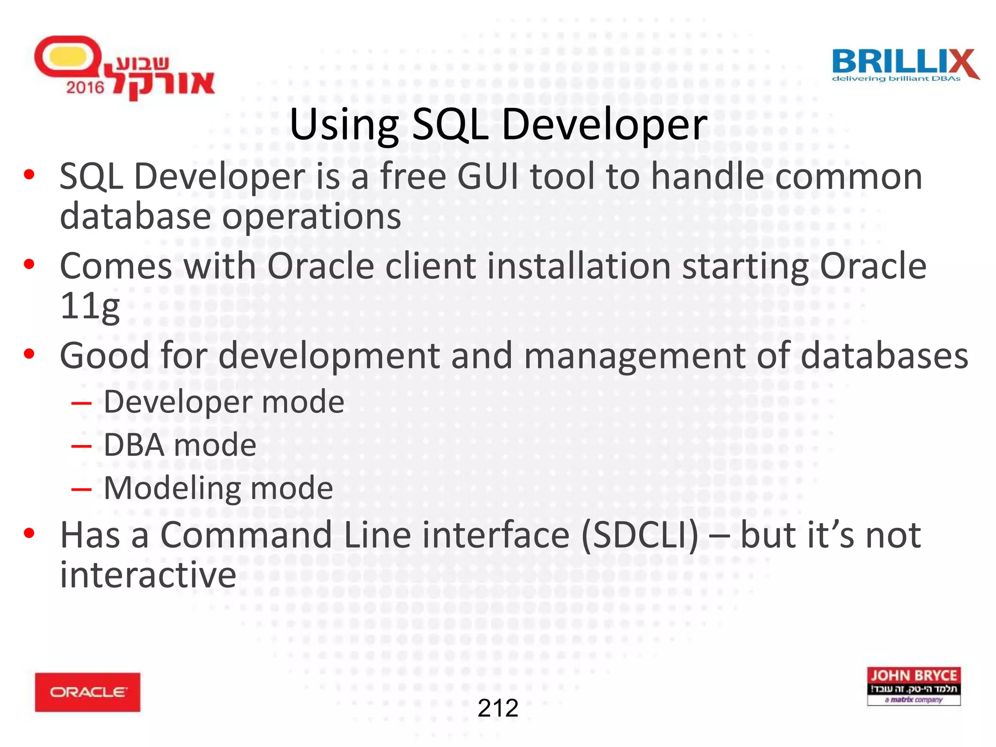
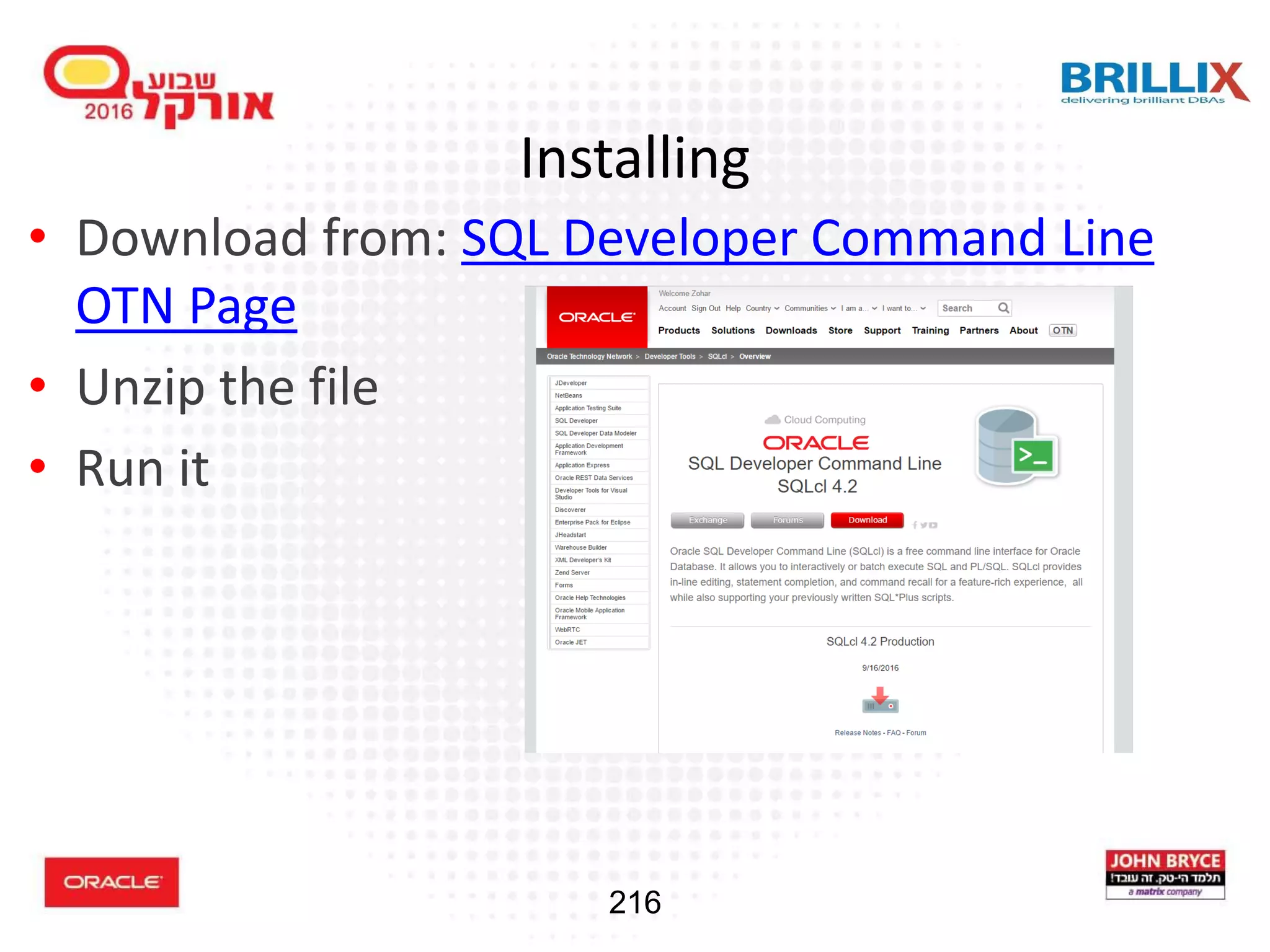
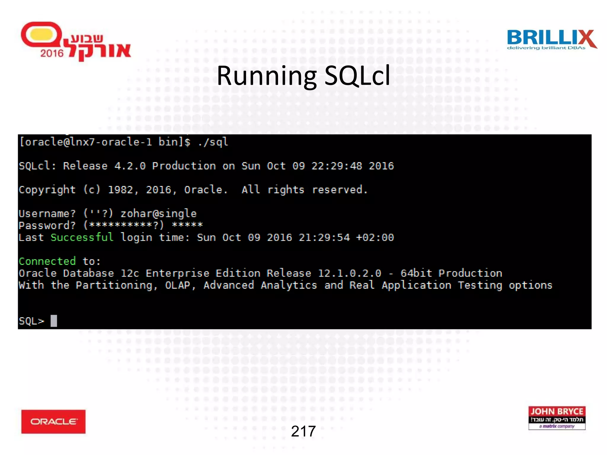
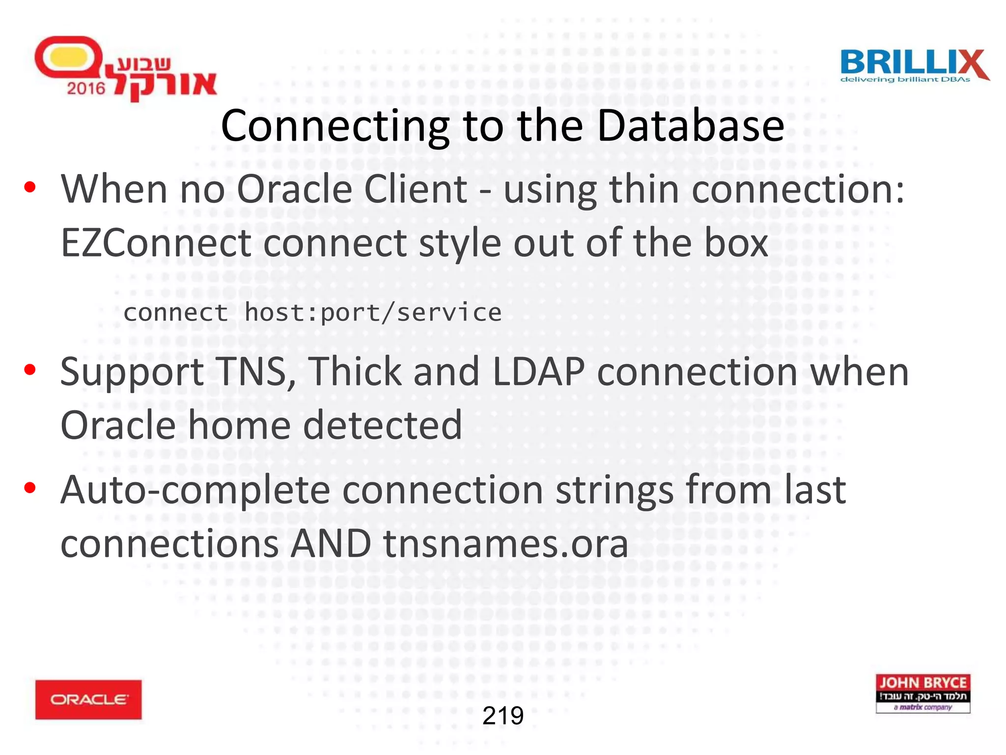
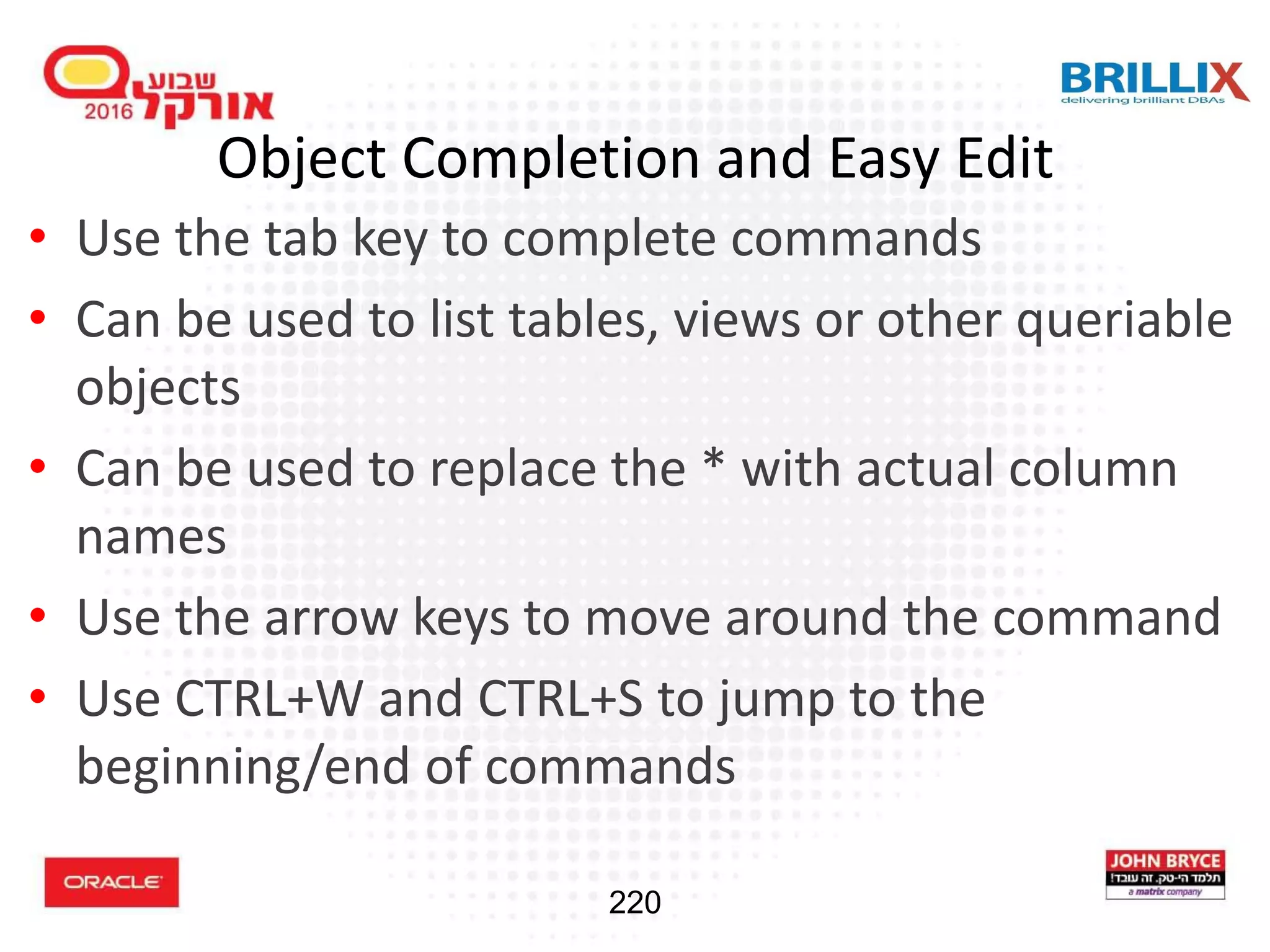
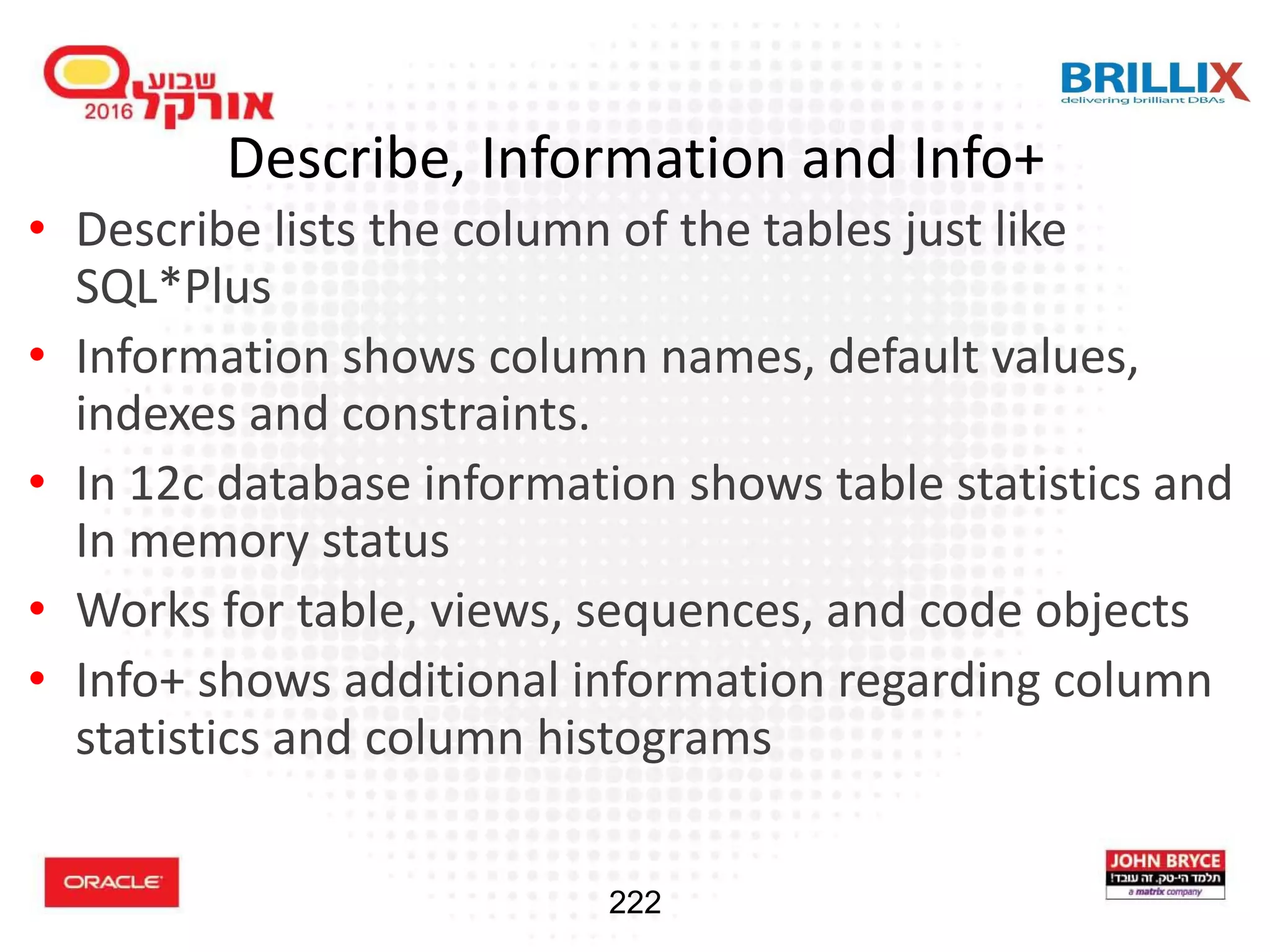
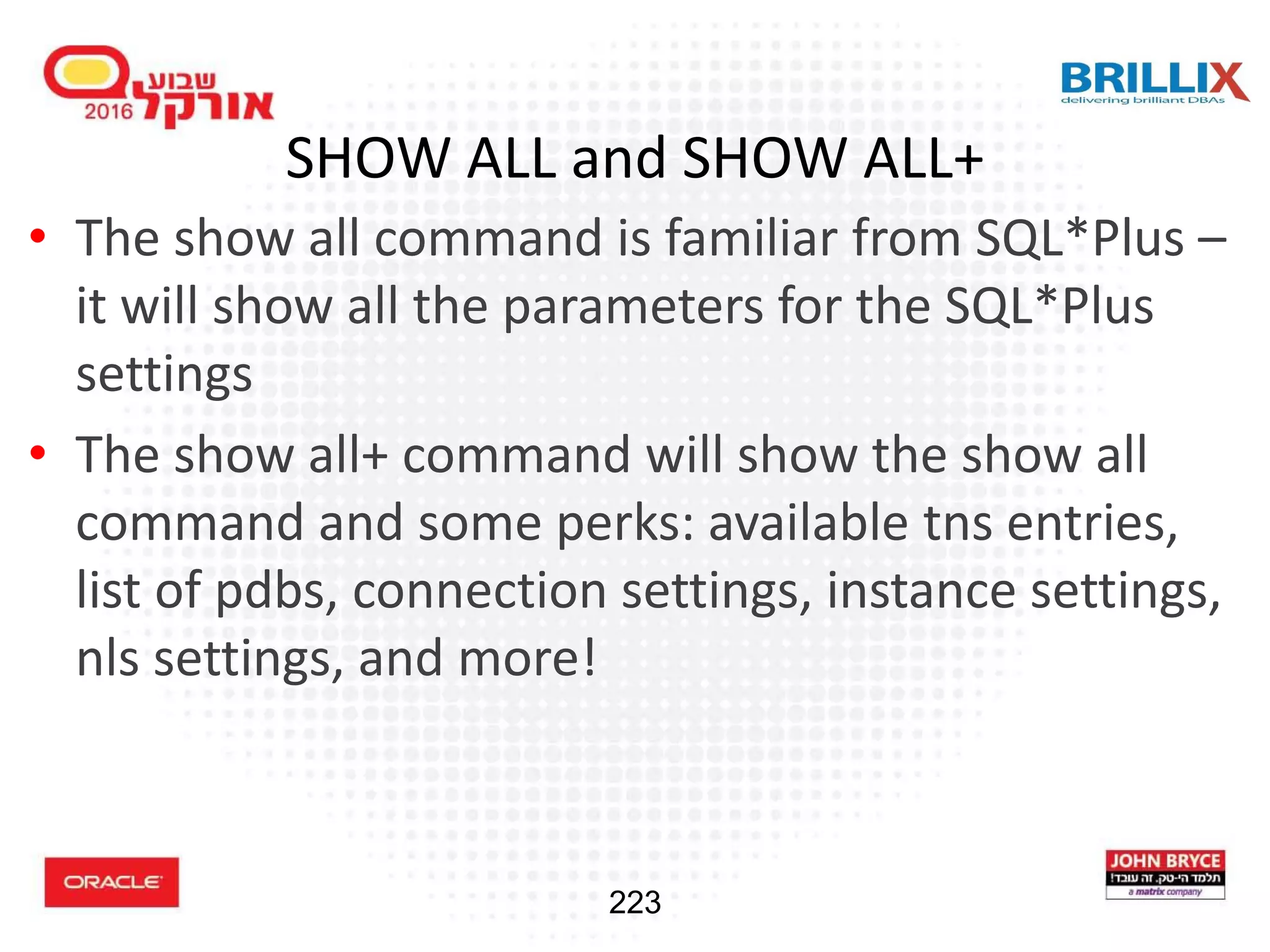
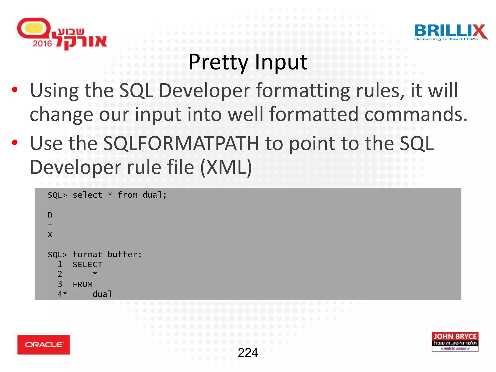
Overview of SQLcl as a modern command line interface to enhance productivity for SQL developers.