Model reduction of unstable systems based on balanced truncation algorithm

Model reduction of unstable systems based on balanced truncation algorithm

• 1.
  International Journal ofElectrical and Computer Engineering (IJECE) Vol. 11, No. 3, June 2021, pp. 2045~2053 ISSN: 2088-8708, DOI: 10.11591/ijece.v11i3.pp2045-2053  2045 Journal homepage: http://ijece.iaescore.com Model reduction of unstable systems based on balanced truncation algorithm Ngoc Kien Vu, and Hong Quang Nguyen Thai Nguyen University of Technology, Thai Nguyen City, Vietnam Article Info ABSTRACT Article history: Received Apr 4, 2020 Revised Sep 5, 2020 Accepted Oct 11, 2020 Model reduction of a system is an approximation of a higher-order system to a lower-order system while the dynamic behavior of the system is almost unchanged. In this paper, we will discuss model order reduction (MOR) strategies for unstable systems, in which the method based on the balanced truncation algorithm will be focused on. Since each MOR algorithm has its strengths and weakness, practical applications should be suitable for each specific requirement. Simulation results will demonstrate the correctness of the algorithms. Keywords: Balanced truncation algorithm High order controller Model order reduction Unstable system This is an open access article under the CC BY-SA license. Corresponding Author: Hong Quang Nguyen Thai Nguyen University of Technology No. 666, 3/2 Street, Thai Nguyen City, Vietnam Email: quang.nguyenhong@tnut.edu.vn 1. INTRODUCTION Model order reduction (MOR) is a method that simplifies higher-order complex models. This is a topic received a lot of attention. However, there still have many issues to be addressed. The balanced truncation (BT) algorithm is one of the most popular methods of order reduction for linear systems. This method was introduced in [1]. Later, the ability to preserve stability during the process of order reduction is proved in [2], and a formula for calculating the error limitation is determined in [3, 4]. In order to perform the BT algorithm, it is necessary to perform the diagonalization process Gramian’s control matrix and Gramian’s observer matrices of the system simultaneously. The equivalence of two diagonal matrices allows transforming the original model represented in any base system to an equivalent base system represented in the coordinate system of internal balanced space. Based on Moore's BT method [1], other algorithms have been proposed such as the random balancing method [5], positive real balance method [6], Hankel standard approximation method [7], etc. Recent studies on the method of BT [8-13] focus on developing or adjusting the BT algorithm corresponding to each specific application. The BT algorithm and other algorithms [14-16] are mainly applied to stable linear systems because the original concepts of the BT method (controllability Gramian and observability Gramian) are always accompanied by the requirement that the system is stable, ie the system has all the poles on the left of the imaginary axis. In practical applications, however, higher-order linear models (higher-order object models, higher-order controllers [17-19]) may be unstable. Therefore, to meet the requirements of the problem of order reduction, algorithms need to be capable to reduce the order of both stable and unstable systems.
• 2.
   ISSN: 2088-8708 IntJ Elec & Comp Eng, Vol. 11, No. 3, June 2021 : 2045 - 2053 2046 To solve the problem of order reduction for unstable systems, there are two strategies:  Strategy 1 (indirect order reduction algorithm): Firstly, the unstable original system is separated into stable and unstable parts. After that, an order reduction algorithm is applied to the stable part [17, 18], [20-23]. Finally, we add the stable reduced-order part with the unstable part.  Strategy 2 (direct order reduction algorithm): In this strategy, order reduction algorithms for stable systems are modified and adjusted so that these algorithms can perform order reduction irrespective of whether the original system is stable or unstable [24-28]. Each of the two above order reduction algorithms has its approach and needs to be evaluated for use in specific applications. To provide a specific evaluation of proposed MOR algorithms for unstable systems, the authors focus on introducing and evaluating algorithms for unstable systems based on Strategy 2. Specifically, we compare three extended BT algorithms for unstable systems: LQG based algorithm [24], Zhou’s BT algorithms [25], and Zilochian BT algorithm [26]. 2. BT BASED ORDER REDUCTION ALGORITHMS FOR UNSTABLE SYSTEMS 2.1. Problem of order reduction Given a linear, continuous, time-invariant system with multiple inputs, multiple outputs, described in the state space as shown in (1): x x u y x    A B C (1) in which, x  Rn , u  Rp , y  Rq , A  Rnxn , B  Rnxp , C  Rqxn . The objective of the problem of order reduction for the model described by (1) is to find the model described by (2): r r r r r r r x x u y x    A B C (2) in which, xr  Rr , u  Rp , yrRq , Ar  Rrxr , Br  Rrxp , Cr  Rqxr , with r  n; so that the model described by (2) can replace the model described by (1), applied to analyze, design, and control the system. 2.2. Zhou’s BT algorithm As mentioned in Section 1, the difficulty of applying the BT algorithm for unstable systems is that the determination of Gramians always comes with the requirement that the original system is asymptotic stable. To determine the Gramians of unstable systems, Zhou [25] proved that special functions X and Y, roots of the two Lyapunov equations, can be used: ' ' 0 ' ' 0       XA A X XBB X AY YA YC CY (3) From the two special functions X and Y by setting F=-B'X and L=-YC', we can determine the controllability Gramian and observability Gramian of the unstable system by two Lyapunov equations as shown in (4):         ' 0 ' ' 0           A BF P P A BF BB Q A LC A A LC C C (4) After determining the controllability Gramian and observability Gramian, we follow steps of Moore's BT algorithm to obtain the reduced-order system of the unstable original system. Detail of Zhou's BT algorithm [25] is as follows: Input : System (A, B, C) described in (1) (unstable system). Step 1: Calculate the special functions X and Y, according to (3). Step 2: Set F=-B'X and L=-YC' Step 3: Calculate the controllability Gramian P and the obsevability Gramian Q, according to (4). Step 4: Analyze the following matrices:
• 3.
  Int J Elec& Comp Eng ISSN: 2088-8708  Model reduction of unstable systems based on… (Ngoc Kien Vu) 2047 Analyze the Cholesky matrix: P=RRT , with R is an upper triangle matrix. Analyze SVD matrix: T T  RQR UΛV . Step 5: Calculate matrix: 1/2 L  V Calculate the singular matrix: 1 -1/2 L T   T R U Step 6: Calculate     1 1 , , , ,    A B C T AT T B CT . Step 7: Select the order that needs to be reduced r so that r < n . Present   , , A B C in a matrix form as follows:   11 12 1 1 2 21 22 2 , , ,                A A B A B C C C A A B In which x x x 11 1 1 , , r r r p q r R R R    A B C . Output: Reduced-order system   11 1 1 , , A B C . 2.3. Zilochian’s extended BT algorithm To overcome the difficulty of identifying Gramians of unstable systems, Zilochian [26] proposed an idea of converting the system from an unstable form to a stable form through coordinate axis displacement (or mapping). When the system is in a stable form, we can reduce the order of the system according to the BT algorithm. Finally, the algorithm performs a reverse projection (reverse displacement of coordinate origin) to convert the stable reduced-order system into an unstable form like the original system. To carry out the idea, the first and crucial step is determining the value of the coordinate axis displacement so that the reduced-order result is an optimal solution. Zilochian [26] demonstrated that the coordinate axis displacement based on the largest-real-part unstable pole has an optimal reduced-order result. The Zilochian’s BT algorithm [26] is stated as below: Input: System (A, B, C) described in (1) (unstable system) with a transfer function:   1 ( ): s s    G C I A B Step 1: Determine the unstable pole  of (1) that has the largest real part. Set real( ) ,      in which R   arbitrary small and 0   . Convert the system (A, B, C) into an unstable system ( ) s  G according to below:         A A I B B C C Step 2: Calculate the observability Gramian  Q and controllability Gramian  P of the system   , ,    A B C by solving two following Liapulov equations: T T T T , .                   A P P A B B A Q Q A C C Step 3: Analyze the following matrices: Analyze the Cholesky matrix: T p p     P R R , with p  R is an upper triangle matrix. Analyze the Cholesky matrix: T o o     Q R R , with o  R is an upper triangle matrix. Analyze SVD matrix: T T o p      R R U ΛV .
• 4.
   ISSN: 2088-8708 IntJ Elec & Comp Eng, Vol. 11, No. 3, June 2021 : 2045 - 2053 2048 Step 4: Calculate the singular matrix  T 1 1/2 p        T R V Λ Step 5: Calculate:     1 1 ˆ ˆ ˆ , , , ,              A B C T A T T B C T Step 6: Select the order that needs to be reduced r so that r < n . Present   ˆ ˆ ˆ , ,    A B C in a matrix form as follows: 11 12 1 1 2 2 21 22 ˆ ˆ ˆ ˆ ˆ ˆ ˆ ˆ , , , ˆ ˆ ˆ                                   A A B A B C C C B A A in which x x x 11 1 1 ˆ ˆ ˆ , , r r r p q r R R R       A B C . We obtain a stable reduced-order system   11 1 1 ˆ ˆ ˆ , ,    A B C . Step 7: Convert stable system   11 1 1 ˆ ˆ ˆ , ,    A B C into  -stable system   11 1 1 ˆ ˆ ˆ , , A B C according to the following equations: 11 11 1 1 1 1 ˆ ˆ , ˆ ˆ , ˆ ˆ .         A A I B B C C Output: Reduced-ordered system   11 1 1 ˆ ˆ ˆ , , A B C 2.4. LQG based BT The idea of the LQG based BT algorithm [24] is that instead of calculating the controllability Gramian and the observability Gramian using Lyapunov equations, the proposed algorithm calculates them using the extended Riccati equation as follows: ' ' ' ' 0 ' ' ' 0         AP PA PC C P BB A Q QA QBB Q C C After determining the controllability Gramian and the observability Gramian, we follow steps of Moore's BT algorithm to obtain the reduced-order system of the unstable original system. Detail of the LQG based BT [24] is as following: Input: System   , , A B C described in (1) (unstable system) Step 1: Calculate the controllability Gramian P and the observability Gramian Q arcording to (11). Step 2: Analyze the following matrixes: Analyze the Cholesky matrix: T  P RR , with R is an upper triangle matrix. Analyze SVD matrix: T T  RQR UΛV . Step 3: Calculate matrix: 1/2 L  V Step 4: Calculate the singular matrix: 1 -1/2 L T   T R U Step 5: Calculte:     1 1 , , , ,    A B C T AT T B CT . Step 6: Select the order need to be reduced r so that r < n .
• 5.
  Int J Elec& Comp Eng ISSN: 2088-8708  Model reduction of unstable systems based on… (Ngoc Kien Vu) 2049 Present   , , A B C in a matrix form as follows:   11 12 1 1 2 21 22 2 , , ,                A A B A B C C C A A B In which x x x 11 1 1 , , r r r p q r R R R    A B C . Output: Reduced-order system   11 1 1 , , A B C . 3. SIMULATION AND DISCUSSION 3.1. Order reduction of high order controller Consisder a 28th order controller as follows: ( ) ( ) ( ) s s s  N R D In which 28 27 26 25 4 24 6 23 7 22 8 21 10 20 11 19 12 18 13 17 14 16 15 15 15 14 1 ( ) 0.004867 0.7519 58.8 2526 8.35.10 2.128.10 4.383.10 7.542.10 1.108.10 1.411.10 s 1.527.10 1.544.10 1.341.10 1.032 7.021.10 4.211.10 s s s s s s s s s s s s s e s s                  N 6 13 17 12 18 11 18 10 19 9 19 8 19 7 20 6 20 5 20 4 19 3 19 2 16 2.213.10 1.01.10 3.954.10 1.306.10 3.564.10 7.845.10 1.348.10 1.723.10 1.52.10 8.162.10 1.984.10 3.89.10 125.2 s s s s s s s s s s s s s              and 5 28 27 26 25 24 4 23 6 22 7 21 8 20 9 19 10 18 12 17 12 16 13 15 14 14 15 13 ( ) 5.25 0.009786 0.8675 48.8 1965 6.056.10 1.49.10 3.018.10 5.14.10 7.483.10 9.425.10 1.035.10 9.968.10 +8.432.10 6.266.10 4.079.10 s e s s s s s s s s s s s s s s s s                 D 16 12 17 11 17 10 18 9 18 8 19 7 19 6 19 5 19 4 19 3 18 2 4 11 2.314.10 1.134.10 4.74.10 1.66.10 4.762.10 1.085.10 1.891.10 2.399.10 2.062.10 1.065.10 2.479.10 1.59.10 2.945.10 s s s s s s s s s s s s               In practice, a 28th order controller has many disadvantages when it comes to real-time control, so order reduction of this controller is a crucial problem. The 28th order controller is a stable linear model but it has two poles that approximately equal to zero. The 28th order controller is used as an object to evaluate the efficiency of order reduction algorithms introduced in section 2. Results are obtained in the following Tables 1-3: Table 1. Results of order reduction for a high-order controller according to Zhou's BT algorithm Order ( ) r s R 5 5 4 3 4 2 4 4 5 4 3 2 2 92.89 .10 . 925.9 6851 4.932 1.635 1.999 42.24 706.8 6955 143 2639 10 .10 s s s s s s s s s s            4 4 3 2 4 4 4 3 2 912.8 6772 4.801 1.106 42.1 701.4 6869 1312 92.89 .10 .10 s s s s s s s s          3 3 2 2 4 3 906.5 4.763.10 .03 696.4 6757 92.89 6518 42 s s s s s s        2 2 2 2 521.2 377 26.66 178.7 92.89 4 s s s s      Note: We will call the reduced-order controller (order of r) is an r-order controller
• 6.
   ISSN: 2088-8708 IntJ Elec & Comp Eng, Vol. 11, No. 3, June 2021 : 2045 - 2053 2050 Table 2. Results of the order reduction of a high-order controller according to Zilochian 's BT algorithm Order ( ) r s R 5 5 4 3 4 2 4 4 5 4 3 2 92.89 438.1 7570 2.603.10 3.759.10 1.26.10 36.85 557.6 4799 4428 1653 s s s s s s s s s s            4 4 3 2 4 4 4 3 2 92.89 424 7535 2.483.10 3.513.10 36.7 552.5 4720 3923 s s s s s s s s          3 2 2 3 4 3 407.5 6853 2.386 6 92.89 538.8 4 .10 736.52 44 s s s s s s        2 2 2 2 220.1 4576 29.11 336.2 92.89s s s s      Table 3. Result of the order reduction of a high-order controller according to LQG based BT Order ( ) r s R 5 5 4 3 4 2 4 5 4 3 2 92.89 .10 .10 36.31 587.8 5599 2845 560.5 7588 3.197 2.632 37.48 0.006441 s s s s s s s s s s            4 4 3 2 4 4 3 2 3.139 65.45 0.01912 92.89 547 7030 .10 36.17 577.1 5360 s s s s s s s s          3 3 2 3 2 +278.7 3.781 29.28 0.003809 92.89 3613 254.1 s s s s s s       2 2 2 2 891.7 0.1328 22.68 -0.0004031 92.89s s s s     3.2. Simulation results and discussion To evaluate and identify an appropriate reduced-order model, step response and frequency response of the original controller and the reduced-order controller will be used. Simulation results are shown in Figures 1-3. (a) (b) Figure 1. Transient response and frequency response of the original controller and the 4th order controller, (a) transient response, and (b) frequency response
• 7.
  Int J Elec& Comp Eng ISSN: 2088-8708  Model reduction of unstable systems based on… (Ngoc Kien Vu) 2051 (a) (b) Figure 2. Transient response and frequency response of the original controller and the 3rd order controller, (a) transient response and (b) frequency response (a) (b) Figure 3. Transient response and frequency response of the original controller and the 2nd order controller, (a) transient response, and (b) frequency response
• 8.
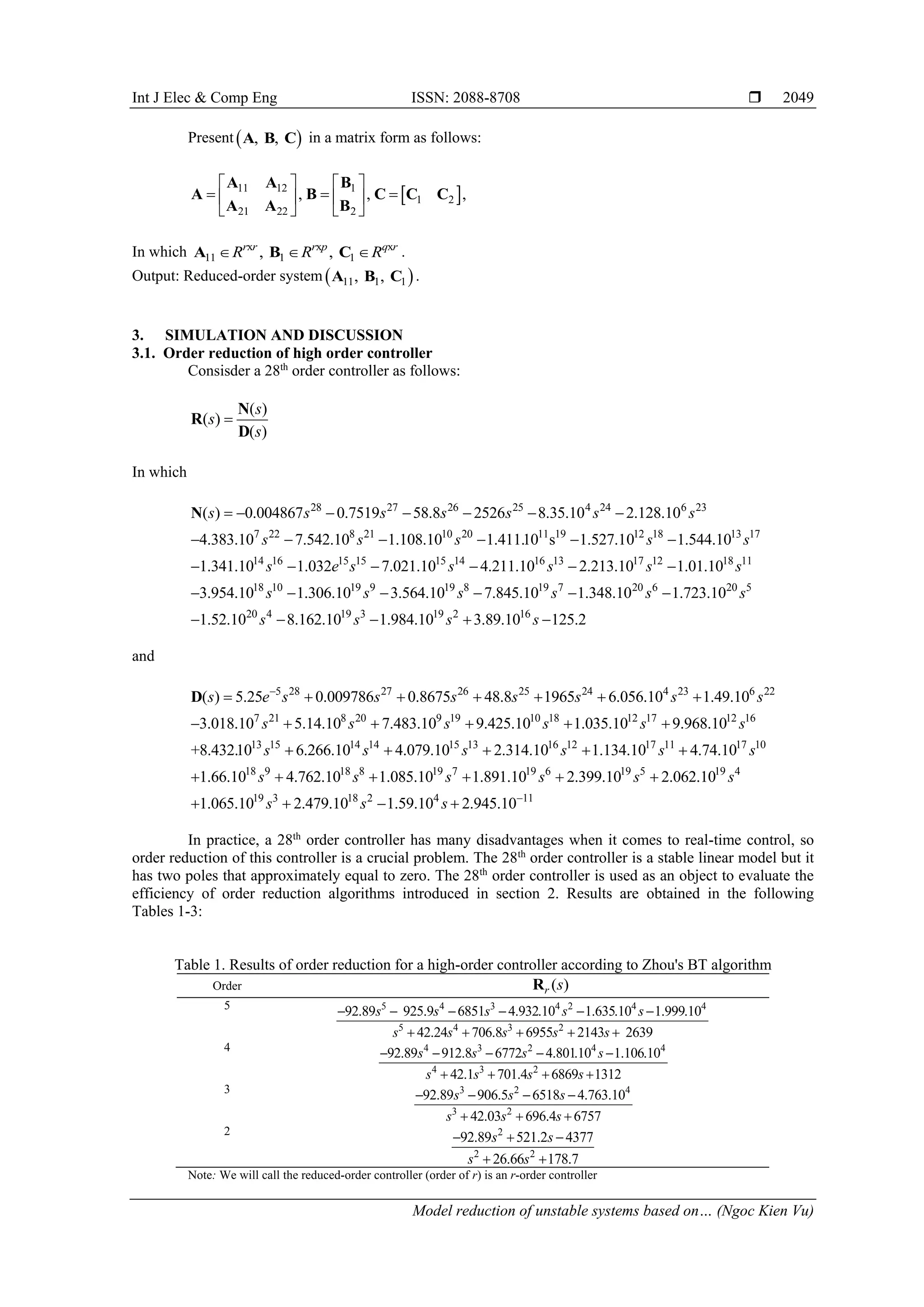
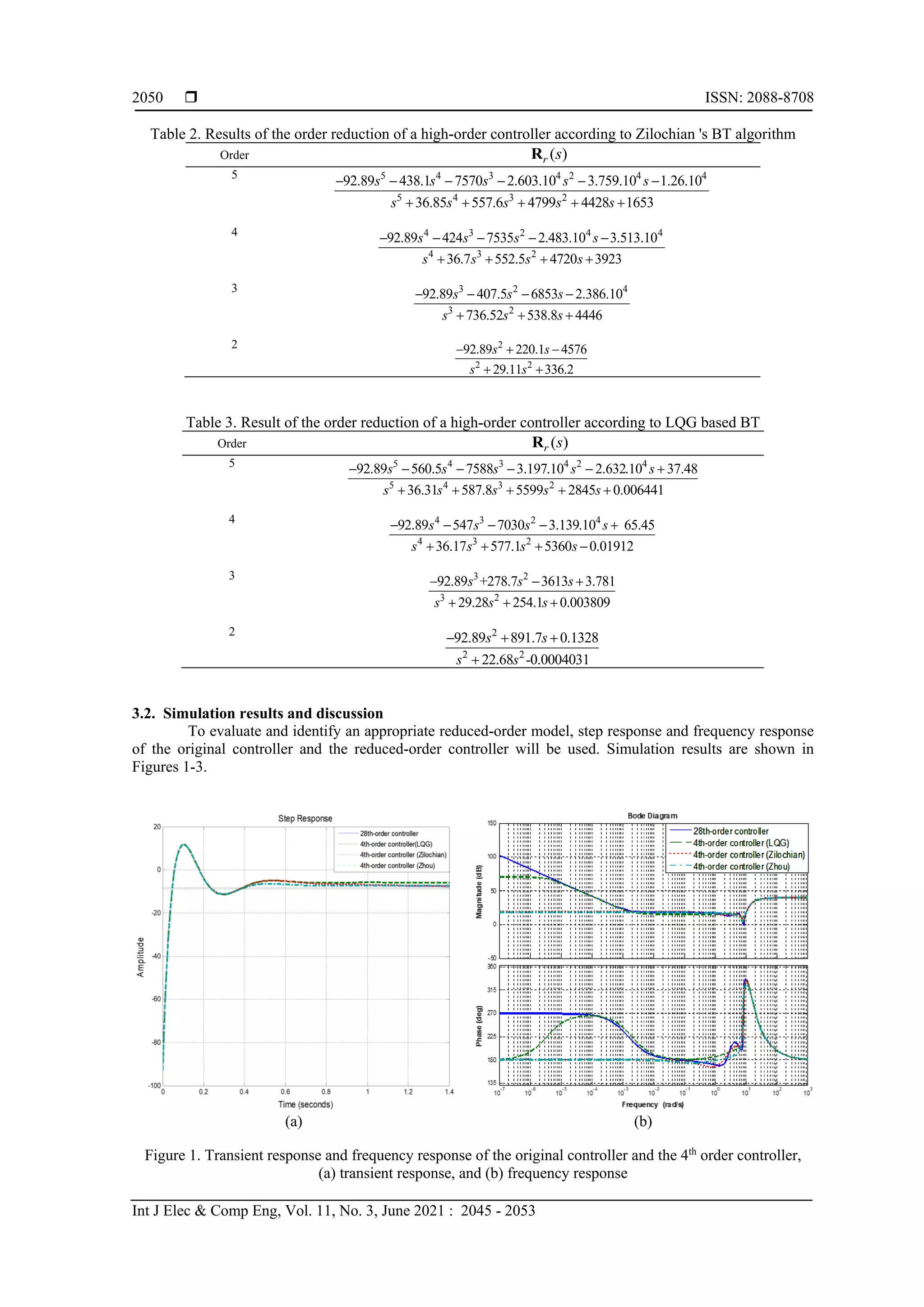
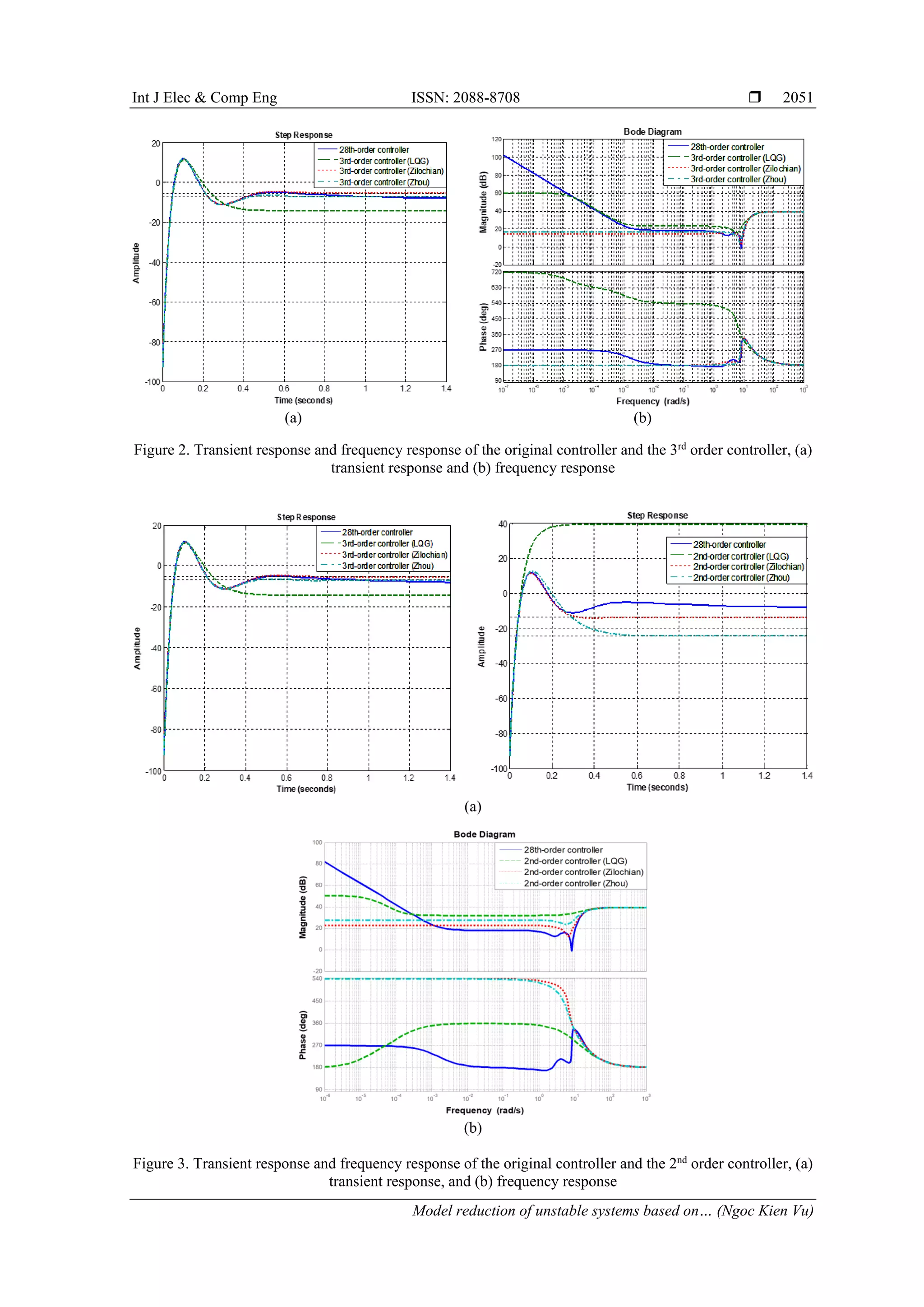
   ISSN: 2088-8708 IntJ Elec & Comp Eng, Vol. 11, No. 3, June 2021 : 2045 - 2053 2052 From simulation results, we see that: a) With transient response:  The transient response of the 4th order controller based on Zilochian’s MOR algorithm is closest to the transient response of the original system among three considered algorithms.  The transient response of the 3rd order controller based on Zhou’s MOR algorithm is closest to the transient response of the original system among three considered algorithms.  The transient responses the second-order controller based on all considered MOR algorithms are much different from the transient response of the original 28th order controller. The second-order controller based on Zilochian’s algorithm has the smallest error among three considered algorithms. b) With frequency response:  The amplitude responses of the 4th, 3rd, and 2nd order controllers according to all three considered algorithms are much different from the amplitude response of the original controller, in which the error of the method based on LQR is smallest. The simulation results of the three methods also show that the lower the order of the controller, the higher the error. c) Through analysis of transient and frequency responses, we see that:  With transient response: reduced-order controllers based on Zilochian’s BT algorithms give the best results (closest to the transients on the original controller).  With frequency response: All reduced-order controller give not good results. (characteristics are much different from the original controller settings). d) From here we see that:  If the requirement of the order reduction problem is mainly concerned with transient response error, we should choose the Zilochian’s MOR algorithm.  If the requirements of the problem of order reduction take into account both transient response and frequency response, we should choose the LQG based algorithm.  Thus, all three direct MOR algorithms are capable of reducing order for unstable systems with their advantages and disadvantages. To choose an appropriate MOR method for unstable systems, we need to base on the requirements set out for the problem of order reduction for unstable systems to select the appropriate algorithm. 4. CONCLUSION The paper has introduced three MOR algorithms for unstable systems based on the BT algorithm. By analyzing these MOR algorithms through illustrative examples, we see that each algorithm has its advantages and disadvantages. From these assessments, we can choose the MOR method under the requirements of the problem of order reduction for unstable systems. Our on-going research direction is to evaluate and compare other indirect MOR algorithms with the three mentioned algorithms and use the results in specific applications to have a more accurate quality evaluation of reduced-order systems. ACKNOWLEDGEMENTS This research was funded by Thai Nguyen University of Technology, No. 666, 3/2 Street, Thai Nguyen City, Viet Nam. REFERENCES [1] Moore B. C., “Principal component analysis in linear systems: Controllability, observability, and model reduction,” IEEE Trans. Auto. Contr., vol. 26, no. 1, pp. 17-32, 1981, doi: 10.1109/TAC.1981.1102568. [2] Perenbo I., and Silverman L. M., “Model reduction via balanced state space repre-sentation,” IEEE Trans. Auto, contr., vol. 27, no. 2, pp. 328-387, 1982, doi: 10.1109/TAC.1982.1102945. [3] Glover K., “All optimal Hankel norm approximation of linear multivariable system and their L2 error bounds,” IEEE Trans. Auto. Contr., vol. 29, no. 6, pp. 1105-1113, 1984, doi: 10.1080/00207178408933239. [4] D. Enns, “Model reduction with balanced realizations: An error bound and a frequency weighted generalization,” Proc. 23rd IEEE Conf. Decision and Control, 1984, doi: 10.1109/CDC.1984.272286. [5] Desai U. B., and Pal D., “A Transformation Approach to Stochastic Model Reduction,” IEEE Transactions on Automatic Control, vol. 29, no. 12, pp. 1097-1100, 1984, doi:10.1109/TAC.1984.1103438. [6] Green M., “A Relative Error Bound for Balanced Stochastic Truncation,” IEEE Trans. Auto. Contr., vol. 33, no. 10, pp. 961-965, 1988, doi:10.1109/9.7255. [7] Antoulas A. C., Sorensen D. C., Gugercin S., “A Survey of Model Reduction Methods for Large-scale Systems,” Structured Matrices in Mathematics, Computer Science, and Engineering, AMS 2001, pp. 193-219, 2001.
• 9.
  Int J Elec& Comp Eng ISSN: 2088-8708  Model reduction of unstable systems based on… (Ngoc Kien Vu) 2053 [8] H. Sandberg, “Model reduction of linear systems using extended balanced truncation,” IEEE American Control Conference, 2008, pp. 4654-4659, doi: 10.1109/ACC.2008.4587229. [9] Heinkenschloss, M., Sorensen, D. C., and Sun, K., “Balanced Truncation Model Reduction for a Class of Descriptor Systems with Application to the Oseen Equations,” SIAM J. Scientific Computing, vol. 30, no. 2, pp. 1038-1063, 2008, doi: 10.1137/070681910. [10] Stykel, T., “Balanced truncation model reduction for semidiscretized Stokes equation,” Linear Algebra Appl., vol. 415, no. 2-3, pp. 262-289, 2006, doi: 10.1016/j.laa.2004.01.015. [11] Duff, I.P., Goyal, P.K., and Benner, P., “Balanced Truncation for a Special Class of Bilinear Descriptor Systems,” IEEE Control Systems Letters, vol. 3, pp. 535-540, 2019, doi:10.1109/LCSYS.2019.2911904. [12] M. G. Safonov and R. Y. Chiang, “A Schur Method for Balanced Model Reduction,” 1988 American Control Conference, 1988, doi: 10.23919/ACC.1988.4789873. [13] Benner P., Hossain MS., Stykel T., “Model Reduction of Periodic Descriptor Systems Using Balanced Truncation,” In: Benner P., Hinze M., ter Maten E. (eds) Model Reduction for Circuit Simulation. Lecture Notes in Electrical Engineering, Springer, Dordrecht, vol. 74, 2011. [14] Hadeel N. Abdullah, “A hybrid bacterial foraging and modified particle swarm optimization for model order reduction,” International Journal of Electrical and Computer Engineering (IJECE), vol 9, no 2, pp. 1100-1109, 2019, doi:10.11591/ijece.v9i2.pp.1100-1109. [15] I. Kasireddy, A. W. Nasir, and A. K. Singh, “Non-integer IMC Based PID Design for Load Frequency Control of Power System through Reduced Model Order,” International Journal of Electrical and Computer Engineering (IJECE), vol. 8, no. 2, pp. 837-844, 2018, doi: 10.11591/ijece.v8i2.pp837-844 [16] D. Srinivasa Rao, M. Siva Kumar, M. Ramalinga Raju, “Design of Robust Controller for Higher Order Interval System Using Differential Evolutionary Algorithm,” International Journal of Robotics and Automation (IJRA), vol. 7, no. 4, pp. 232-250, 2019, doi: 10.11591/ijra.v7i4.pp232-250. [17] Cong Huu Nguyen, Kien Ngoc Vu, and Hai Trung Do, “Model reduction based on triangle realization with pole retention,” Applied Mathematical Sciences, vol. 9, 2015, no. 44, pp. 2187-2196, 2015, doi: 10.12988/ams.2015.5290. [18] Kiki Mustaqim, Didik Khusnul Arif, Erna Apriliani and Dieky Adzkiya, “Model reduction of unstable systems using balanced truncation method and its application to shallow water equations,” Journal of Physics: Conference Series, vol. 855, no. 1, 2017. [19] Rodríguez, D. F., Cuellar, B. D., Sename, O., and Villa, M. V., “On the stabilization of high order systems with two unstable poles plus time delay,” 20th Mediterranean Conference on Control & Automation (MED), 2012, doi: 10.1109/MED.2012.6265607. [20] C.S. Hsu and D. Hou, “Reducing unstable linear control systems via real schur transformation,” Electron. Lett., pp. 984-986, 1991, doi: 10.1049/el:19910614. [21] S. K. Nagar and S. K. Singh, “An algorithmic approach for system dedcomposition and balanced realized model reduction,” J. of Franklin Inst., vol. 341, pp. 615-630, 2004, doi: 10.1016/j.jfranklin.2004.07.005 [22] Varga, “Model reduction software in the slicot library,” Applied and Computational Control, Signals and Circuits, vol. 629, pp. 239-282, 2001. [23] Fatmawati, Saragih, R., Bambang, R. T., and Soeharyadi, Y., “Balanced truncation for unstable infinite dimensional systems via reciprocal transformation,” International Journal of Control, Automation and Systems, vol. 9, pp. 249-257, 2011. [24] Jonckheere E. A., Silverman L. M., “A New Set of Invariants for Linear System-Application to Reduced Order Compensator Design,” IEEE Transactions on Automatic Control, AC- 28, no. 10, pp. 953-964, 1983. [25] Zhou K., Salomon G., Wu E., “Balanced realization and model reduction method for unstable systems,” International Journal of Robust and Nonlinear Control, vol. 9, no. 3, pp. 183-198, 1999. [26] Zilochian A., “Balanced Structures and Model Reduction of Unstable Systems,” IEEE Proceedings of Southeastcon 91, vol 2, pp. 1198-1201, 1991. [27] Boess, C., Nichols, N., Bunse-Gerstner, A., “Model reduction for discrete unstable control systems using a balanced truncation approach,” Preprint MPS, University of Reading, 2010. [28] Boess, C., Lawless, A., Nichols, N., Bunse-Gerstner, A., “State estimation using model order reduction for unstable systems,” Comput. Fluids, vol. 36, no. 1, pp. 155-160, 2011, doi: 10.1016/j.compfluid.2010.11.033.