Data Preprocessing Lecture 2
Data Types
Categorical Data
Categorical Data
Text Data
Pre-processing in NLP
What is Data Preprocessing • Data preprocessing is a process of preparing the raw data and making it suitable for a machine learning • It is the first and crucial step while creating a machine learning model. Why do we need Data Preprocessing • A real-world data generally contains • Noises • missing values • It maybe in an unusable format which cannot be directly used for machine learning models.
Steps for data preprocessing • Acquire the dataset • Import all the crucial libraries • Import the dataset • Identifying and handling the missing values • Encoding the categorical data • Splitting the dataset • Feature scaling
Acquiring the dataset • The first step in data preprocessing in machine learning • The dataset will be comprised of data gathered from multiple and disparate sources which are then combined in a proper format to form a dataset • Dataset formats differ according to use cases. • A business dataset will be entirely different from a medical dataset. • A business dataset will contain relevant industry and business data • A medical dataset will include healthcare-related data. • Once the dataset is ready, you must put it in CSV, or HTML, or XLSX file formats. https://www.kaggle.com/datasets https://archive.ics.uci.edu/ml/index.php
Importing the libraries • Numpy • It is the fundamental package for scientific calculation in Python. • It is used for inserting any type of mathematical operation in the code. • Also used to add large multidimensional arrays and matrices in your code. • Pandas • Pandas is an open-source Python library for data manipulation and analysis. • It is used for importing and managing the datasets. • Matplotlib • Matplotlib is a Python 2D plotting library that is used to plot any type of charts in Python.
Code:
Sample dataset • For our exercise the dataset is given in Data.csv file • It has 10 instances/examples • It has three independent variables • Country • Age • Salary • It has one dependent variable • Purchased • Two values are missing • One in Age independent variable • One in Salary independent variable • One variable is categorical i.e., Country
Importing the dataset Code: • Save your Python file in the directory containing the dataset. • read_csv()” is function of the Pandas library. This function can read a CSV file • For every Machine Learning model, it is necessary to separate the independent variables and dependent variables in a dataset. • To extract the independent variables, you can use “iloc[ ]” function of the Pandas library.
Identifying and handling missing values
Identifying and handling missing values • In data preprocessing, it is pivotal to identify and correctly handle the missing values, • Failing to handle missing values, you might draw inaccurate and faulty conclusions and inferences from the data. • There are two commonly used methods to handle missing data: (Ask the domain expert, which method to use) • Deleting a particular row • Impute the data • Replacing with the mean • Replacing with the median • Replacing with the most frequently occurring value • Replacing with a constant value
Deleting a particular row • You remove a specific row that has a null value for a feature or a particular column where more than 75% of the values are missing. • However, this method is not 100% efficient, and it is recommended that you use it only when the dataset has adequate samples. • You must ensure that after deleting the data, there remains no addition of bias.
Code: Deleting rows with nan values
Impute data • This method can add variance to the dataset, and any loss of data can be efficiently negated. • Hence, it yields better results compared to the first method (omission of rows/columns)
Code: Replacing nan values Replacing nan values (most frequent) Replacing nan values (median/mean)
Encoding the data
Encoding the data • Categorical data refers to the information that has specific categories within the dataset. • Machine Learning models are primarily based on mathematical equations. • Thus, you can intuitively understand that keeping the categorical data in the equation will cause certain issues since you would only need numbers in the equations. • How to encode • categorical data • Ordinal data mapping • One hot encoding (nominal data) • Continuous data • Binning • Normalization
Mapping (Ordinal data) • The categorical columns are • eye_color (Nominal) • Satisfaction (Ordinal) • Upsell (Nominal) • The column satisfaction is ordinal. • Since order matters in this column
Mapping (Ordinal data) Code: Satisfaction satisfied very satisfied not satisfied very satisfied slightly satisfied Satisfaction 1 3 0 3 2 Satisfaction very satisfied 3 slightly satisfied 2 satisfied 1 not satisfied 0
One hot encoding (Nominal Data) • Nominal data is not ordered • If we map nominal data as ordinal data, the ML model may assume that there is come some correlation between the nominal variables, thereby producing faulty output. • What is the solution? • To eliminate this issue, we will now use Dummy Encoding. • Dummy variables are those that take the values 0 or 1 to indicate the absence or presence of a specific categorical effect that can shift the outcome. • The value 1 indicates the presence of that variable in a particular column while the other variables become of value 0. • In dummy encoding, the number of columns equals the number of categories.
`one-hot encoding
One Hot encoding
• For the second categorical variable, that is, purchased, you can use the “labelencoder” object of the LableEncoder class. • We are not using the OneHotEncoder class since the purchased variable only has two categories yes or no, both of which are encoded into 0 and 1.
Splitting the dataset • Every dataset for Machine Learning model must be split into two separate sets – • training set • test set. • This is one of the crucial steps of data preprocessing as by doing this, we can enhance the performance of our machine learning model. • Suppose, if we have given training to our machine learning model by a dataset and we test it by a completely different dataset. Then, it will create difficulties for our model to understand the correlations between the models. • Training Set • Training set denotes the subset of a dataset that is used for training the machine learning model. • In the training set, you are already aware of the output. • Test Set • A test set, is the subset of the dataset that is used for testing the machine learning model. • The ML model uses the test set to predict outcomes and evaluate the trained ML model
• Usually, the dataset is split into 70:30 ratio or 80:20 ratio. • 70:30 ratio • This means that you take 70% of the data for training the model while leaving out the rest 30%. • 80:20 ratio • This means that you take 80% of the data for training the model while leaving out the rest 20%.
• The code includes four variables: • X_train – features for the training data • X_test – features for the test data • y_train – dependent variables for training data • y_test – independent variable for testing data • The train_test_split() function includes four parameters, • The first two of which are for arrays of data. • The test_size function specifies the size of the test set. The test_size maybe 0.5, 0.3, or 0.2 – this specifies the dividing ratio between the training and test sets. • The last parameter, “random_state” sets seed for a random generator so that the output is always the same if it is set to zero.
Encoding the continuous data
Feature Scaling (Normalization) and binning • Feature scaling and binning marks the end of the data preprocessing in Machine Learning. Feature Scaling • It is a method to standardize the independent variables of a dataset within a specific range. • In other words, feature scaling limits the range of variables so that you can compare them on common grounds. • It prevents algorithms from being influenced by higher values
Feature Scaling • In the dataset, you can notice that the age and salary columns do not have the same scale. • In such a scenario, if you compute any two values from the age and salary columns, the salary values will dominate the age values and deliver incorrect results. • Thus, we must remove this issue by performing feature scaling for Machine Learning.
Feature Scaling • You can perform feature scaling in Machine Learning in two ways: • Standardization • Normalization • Standardization • Min-Max Normalization
Standardization code • To standardize the data of the test set, mean and standard deviation values of the training set are used. So, there is no data leaking. • Hence, we only use the transform() function for the test set instead of the fit_transform() function.
• Using the above code we get the following standardized data for the train and test data set Training data Test data
Min Max normalization code • To standardize the data of the test set, max and min values of the training set are used. So, there is no data leaking. • Hence, we only use the transform() function for the test set instead of the fit_transform() function.
• Using the above code we get the following min-max normalized data for the train and test data set Training data Test data
Data Binning
• Data binning/bucketing groups data in bins/buckets, in the sense that it replaces values contained into a small interval with a single representative value for that interval. • Sometimes binning improves accuracy in predictive models. • Binning can be applied to • convert numeric values to categorical values • binning by distance • binning by frequency • Reduce numeric values • quantization (or sampling)
• Binning is a technique for data smoothing. • Data smoothing is employed to remove noise from data. • Three techniques are used for data smoothing: • binning • regression • outlier analysis • We will cover only binning here
Example: cupcake • Google trends • Shows the search trends of cupcakes in the world. • Code:
Binning by distance • Import the dataset • Compute the range of values and find the edges of intervals/bins • Define labels • convert numeric values into categorical labels • Plot the histogram to see the distribution
Binning by distance • In this case we define the edges of each bin • We group values related to the column into • Small • Medium • Big • We need to calculate the intervals within which each group falls. • We calculate the interval range as the difference between the maximum and minimum value and then we split this interval into “N=3” parts, one for each group.
• Now we can calculate the range of each interval, i.e. the minimum and maximum value of each interval. • Since we have 3 groups, we need 4 edges of intervals (bins): • small — (edge1, edge2) • medium — (edge2, edge3) • big — (edge3, edge4)
• Now we define the labels • Convert the numeric values of the column into the categorical values
• We can plot the distribution of values by plotting the histogram • If we define the edges of each bin manually
Binning by frequency • Binning by frequency calculates the size of each bin so that each bin contains the (almost) same number of observations, but the bin range will vary. • Steps are as follows • Import the dataset • Define the labels • Use qcut of the pandas library for data binning • Plot the histogram to see the distribution
Binning by Sampling • Sampling is another technique of data binning. • It permits to reduce the number of samples, by grouping similar values or contiguous values. • There are three approaches to perform sampling: • binning by mean: • Each value in a bin is replaced by the mean value of the bin. • Binning by median: • Each bin value is replaced by its bin median value. • Binning by boundary: • each bin value is replaced by the closest boundary value, i.e. maximum or minimum value of the bin.
Binning by mean • Import the dataset • Compute the range of each bin and compute the mean of each bin • Compute the bin edges of each bin • Set the value of each bin to the mean value • Plot the distribution
• Now we should approximate each value of the column to the median value of the corresponding bin • The left edges starts from the beginning of the bin edges and do not contain the last value of the bin edges. • The right edges instead, start from the second value of the bin edges and last until the last value.
• We can quantize the column by defining a function which loops through the intervals and when it finds the correct interval, it returns the mid value.
California Housing Data
NIST Data (Images)
Generate Data

Lecture 2 - Data Pre - Processing.pdf

  • 1.
  • 2.
  • 8.
  • 9.
  • 12.
  • 14.
  • 18.
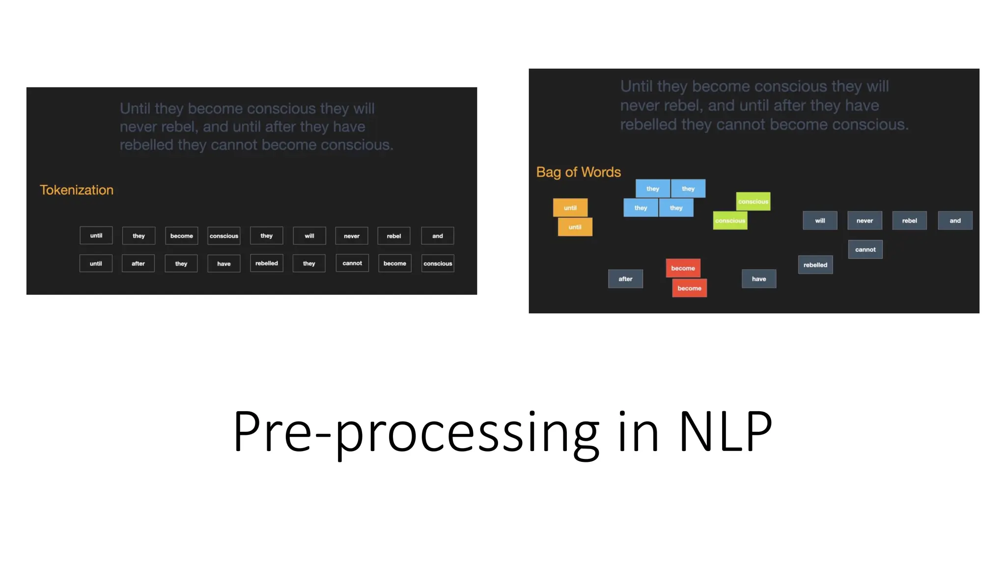
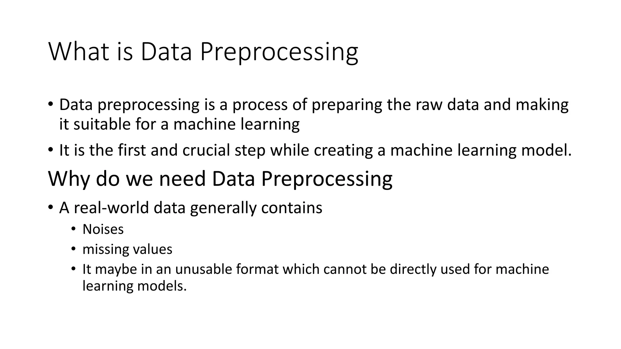
    What is DataPreprocessing • Data preprocessing is a process of preparing the raw data and making it suitable for a machine learning • It is the first and crucial step while creating a machine learning model. Why do we need Data Preprocessing • A real-world data generally contains • Noises • missing values • It maybe in an unusable format which cannot be directly used for machine learning models.
  • 19.
    Steps for datapreprocessing • Acquire the dataset • Import all the crucial libraries • Import the dataset • Identifying and handling the missing values • Encoding the categorical data • Splitting the dataset • Feature scaling
  • 20.
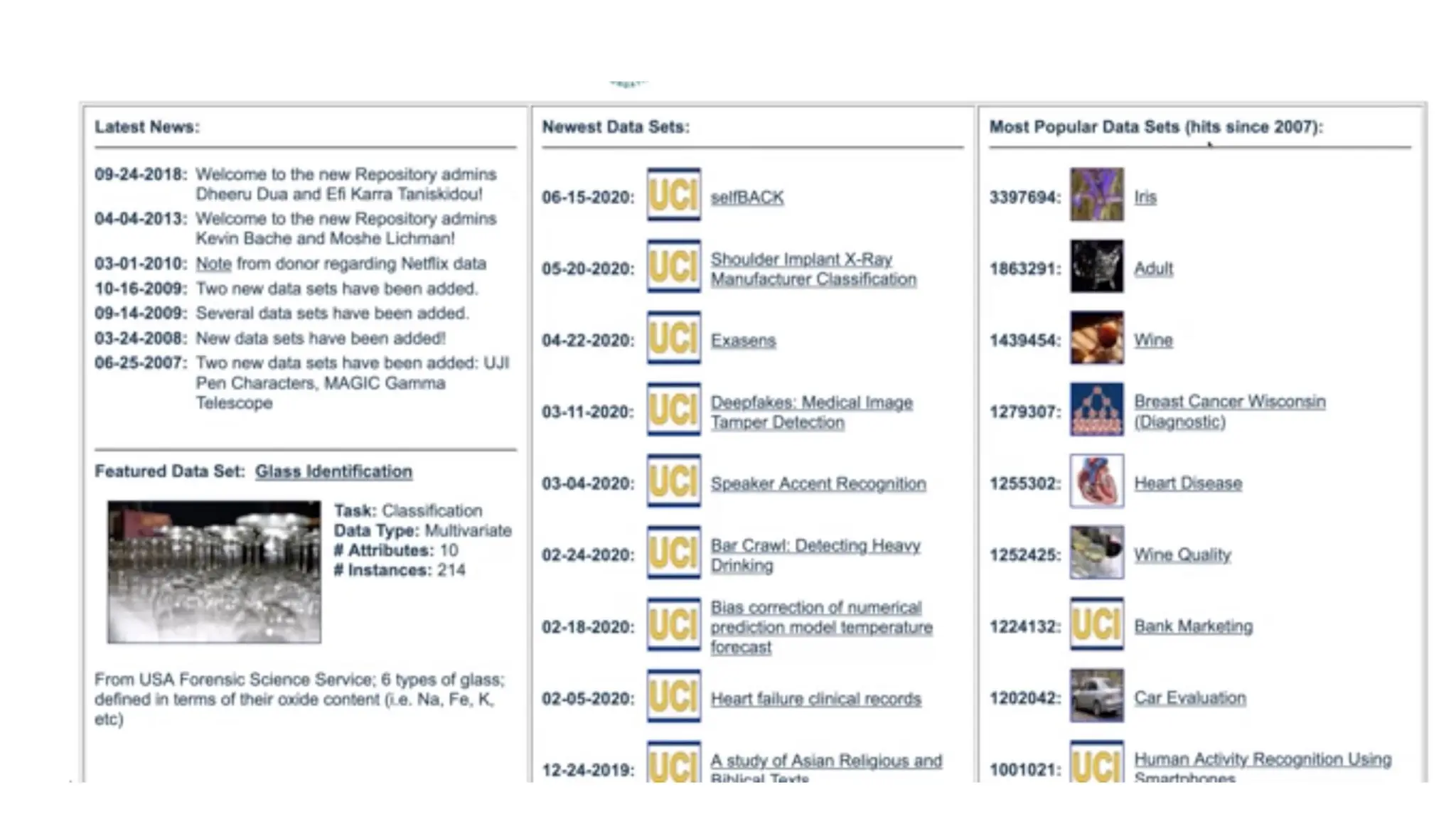
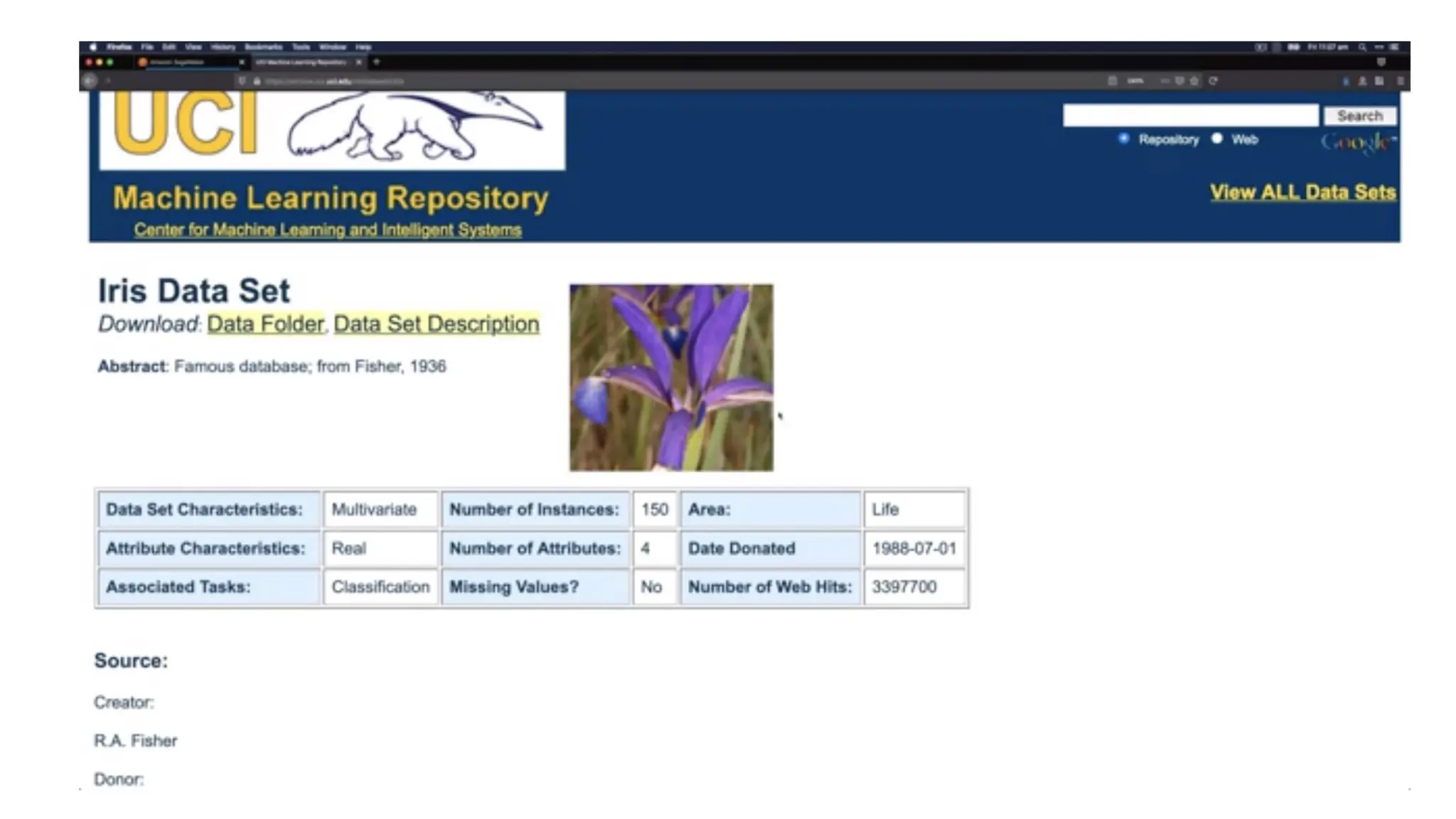
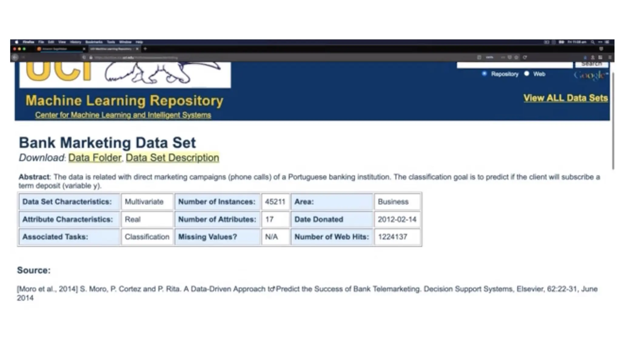
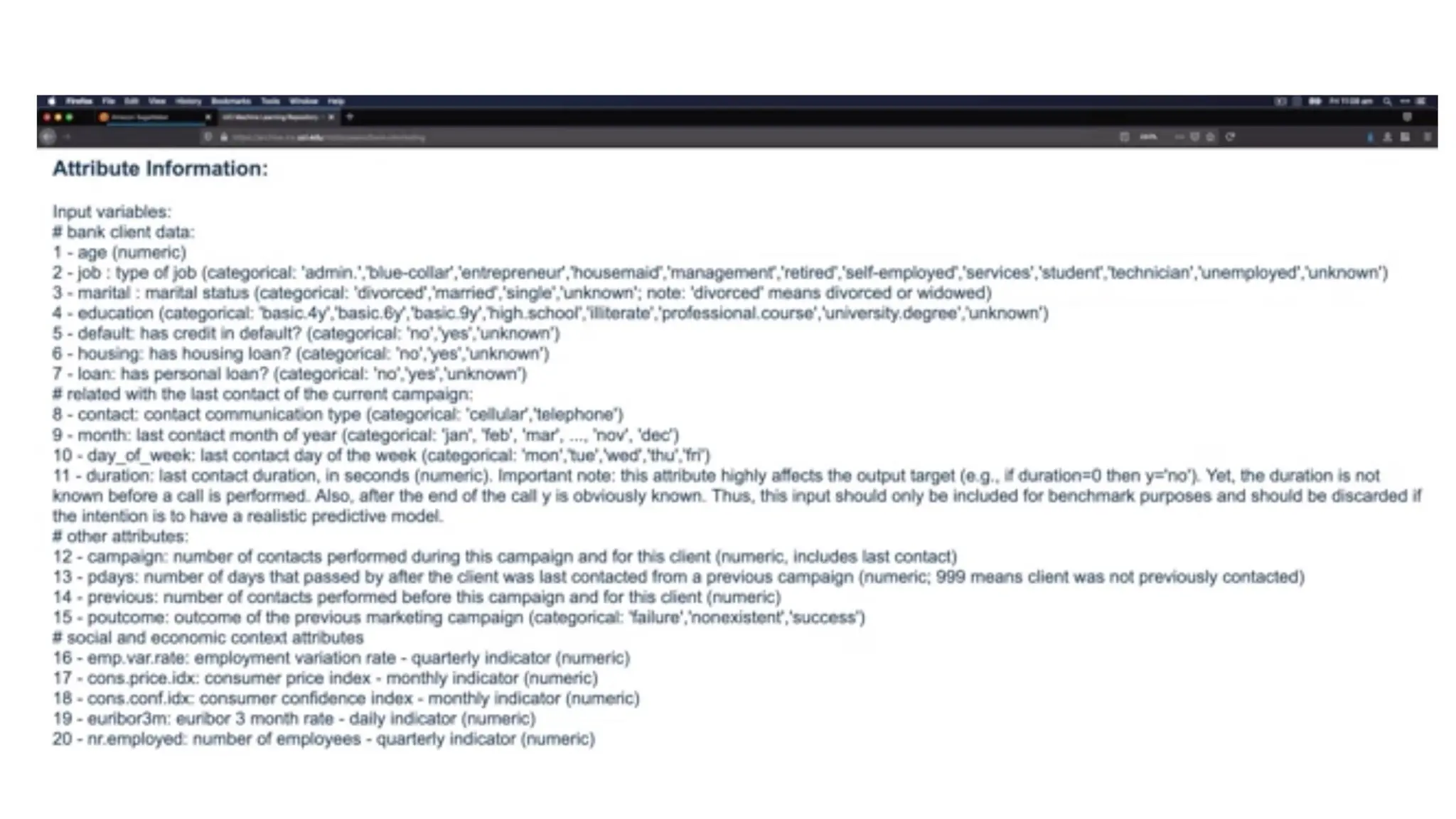
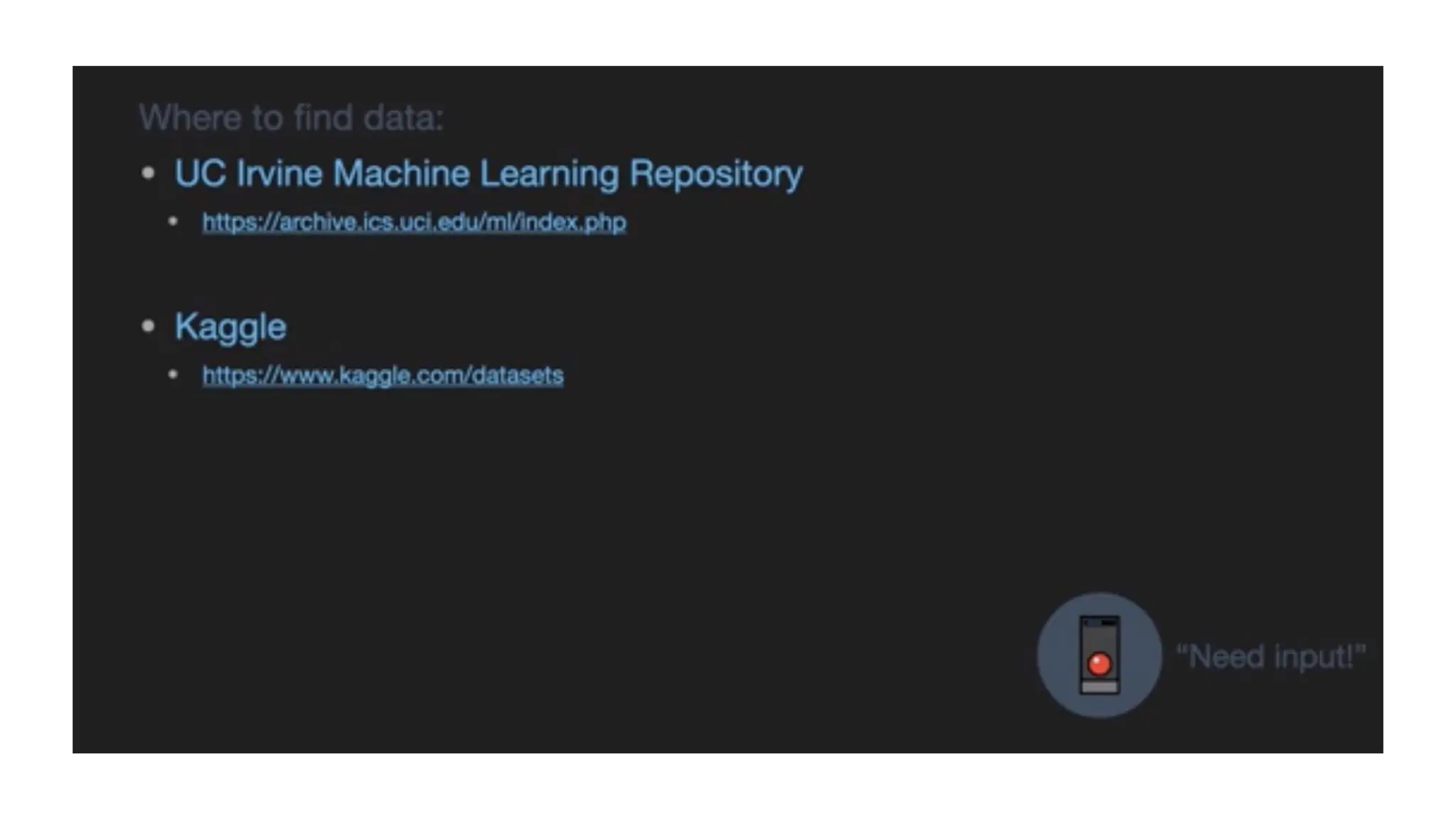
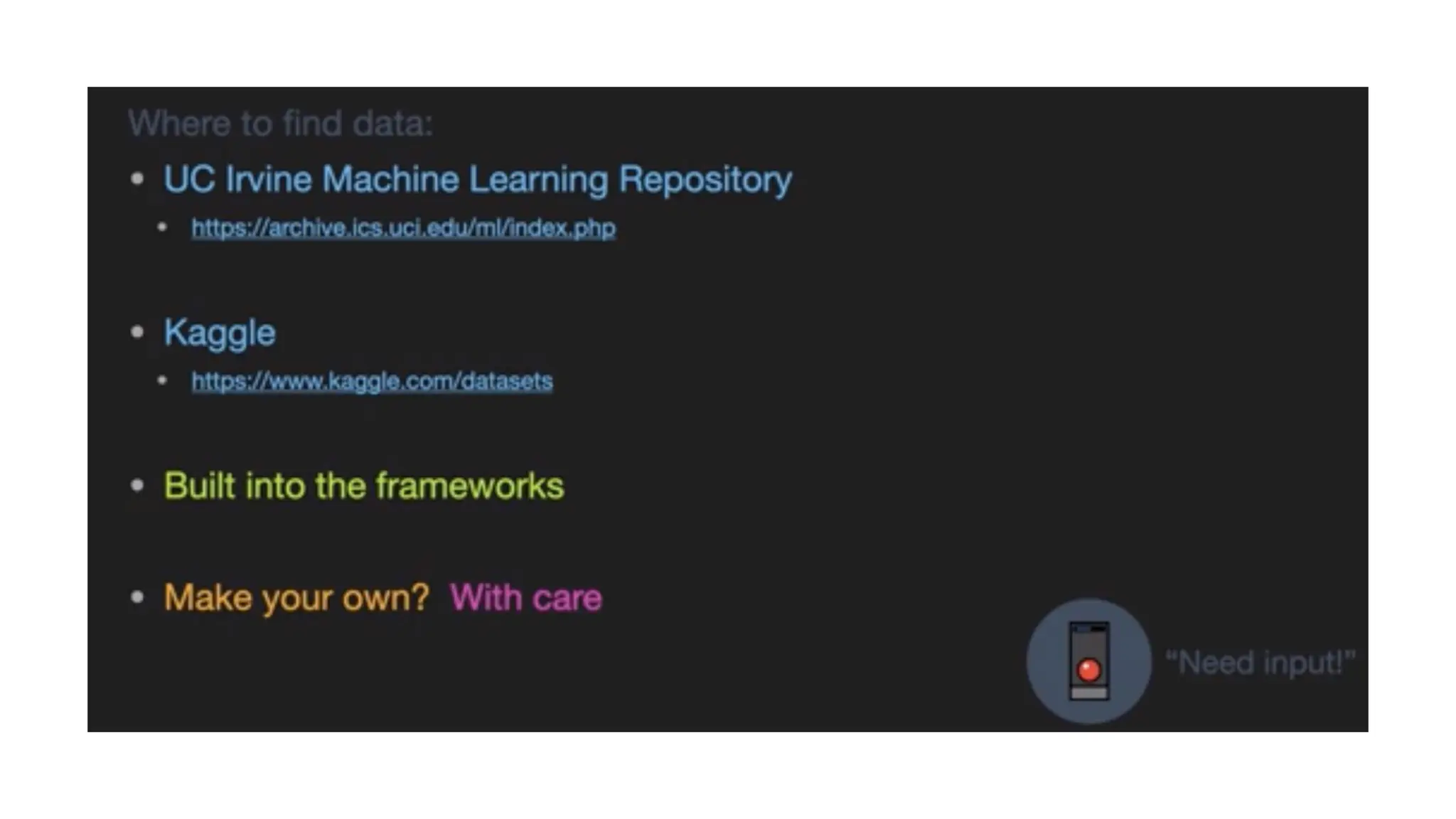
    Acquiring the dataset •The first step in data preprocessing in machine learning • The dataset will be comprised of data gathered from multiple and disparate sources which are then combined in a proper format to form a dataset • Dataset formats differ according to use cases. • A business dataset will be entirely different from a medical dataset. • A business dataset will contain relevant industry and business data • A medical dataset will include healthcare-related data. • Once the dataset is ready, you must put it in CSV, or HTML, or XLSX file formats. https://www.kaggle.com/datasets https://archive.ics.uci.edu/ml/index.php
  • 21.
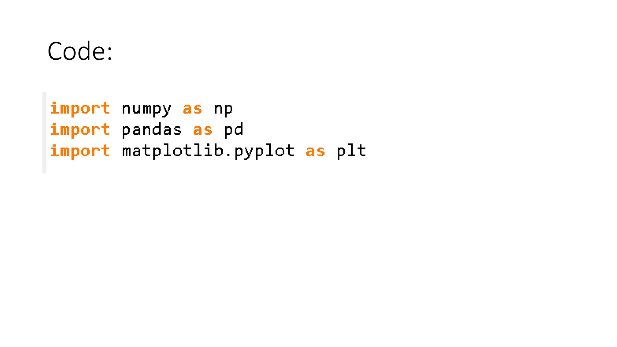
    Importing the libraries •Numpy • It is the fundamental package for scientific calculation in Python. • It is used for inserting any type of mathematical operation in the code. • Also used to add large multidimensional arrays and matrices in your code. • Pandas • Pandas is an open-source Python library for data manipulation and analysis. • It is used for importing and managing the datasets. • Matplotlib • Matplotlib is a Python 2D plotting library that is used to plot any type of charts in Python.
  • 22.
  • 23.
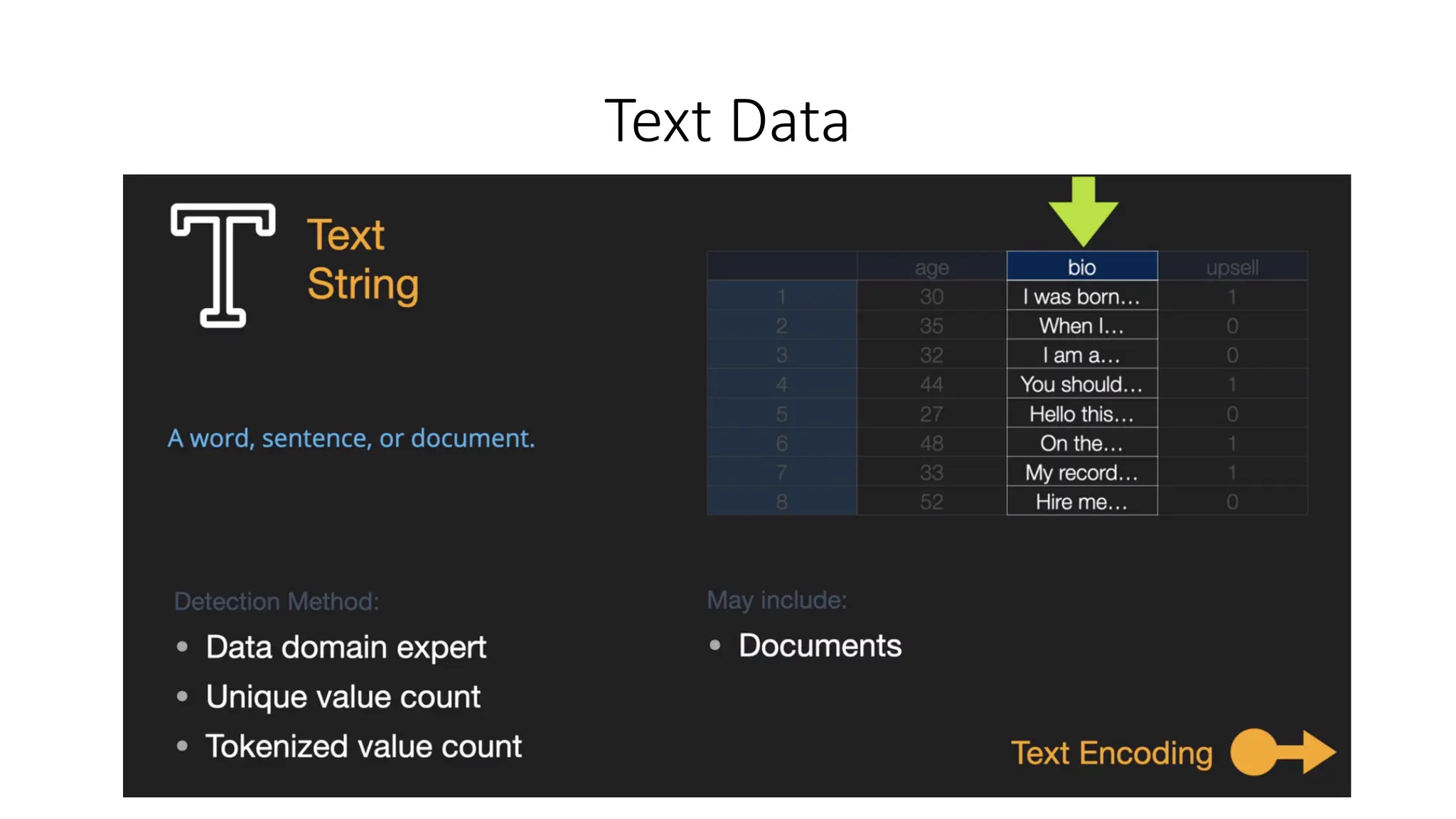
    Sample dataset • Forour exercise the dataset is given in Data.csv file • It has 10 instances/examples • It has three independent variables • Country • Age • Salary • It has one dependent variable • Purchased • Two values are missing • One in Age independent variable • One in Salary independent variable • One variable is categorical i.e., Country
  • 24.
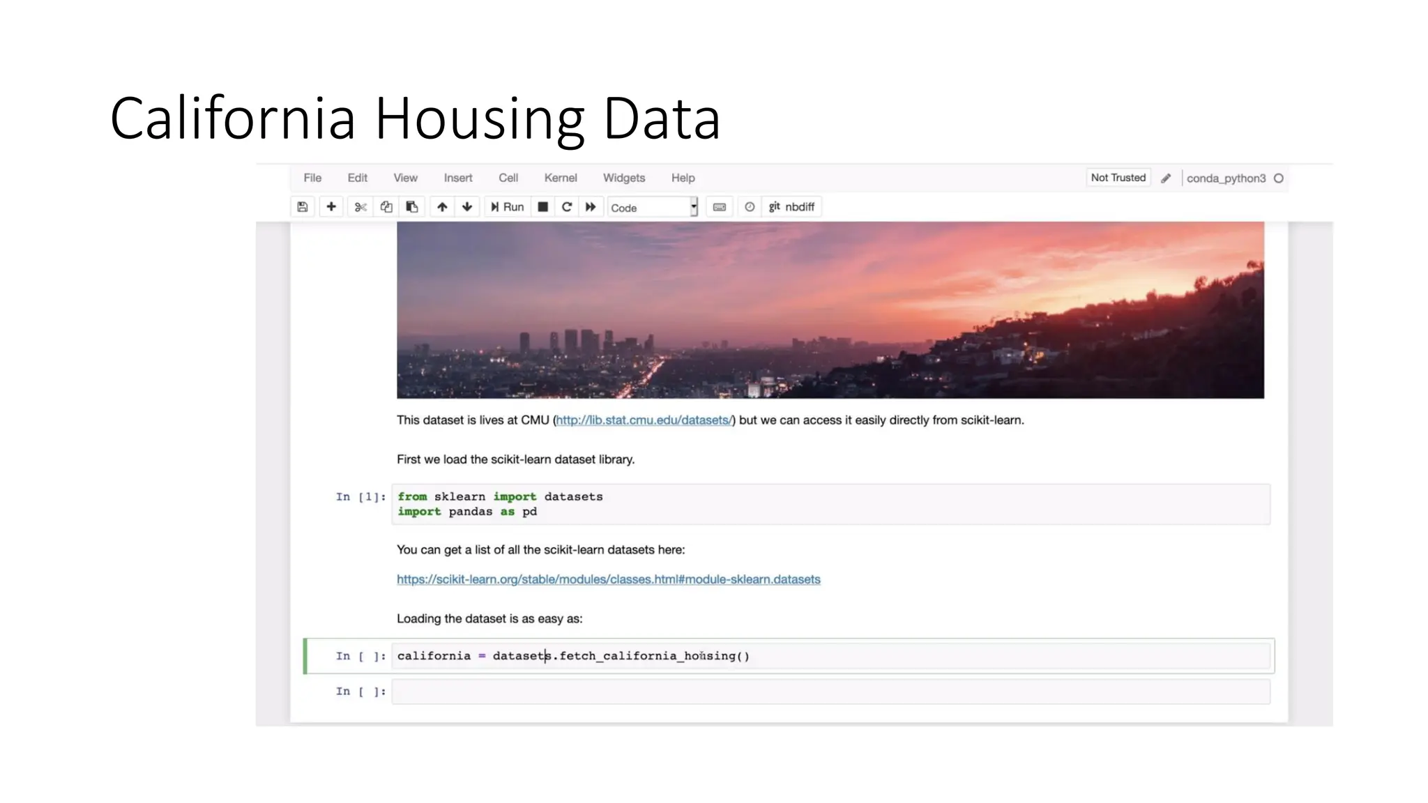
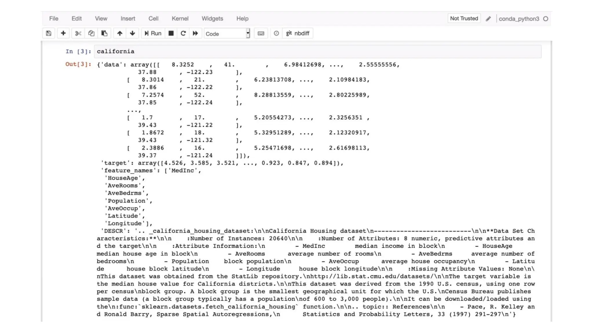
    Importing the dataset Code:• Save your Python file in the directory containing the dataset. • read_csv()” is function of the Pandas library. This function can read a CSV file • For every Machine Learning model, it is necessary to separate the independent variables and dependent variables in a dataset. • To extract the independent variables, you can use “iloc[ ]” function of the Pandas library.
  • 25.
  • 27.
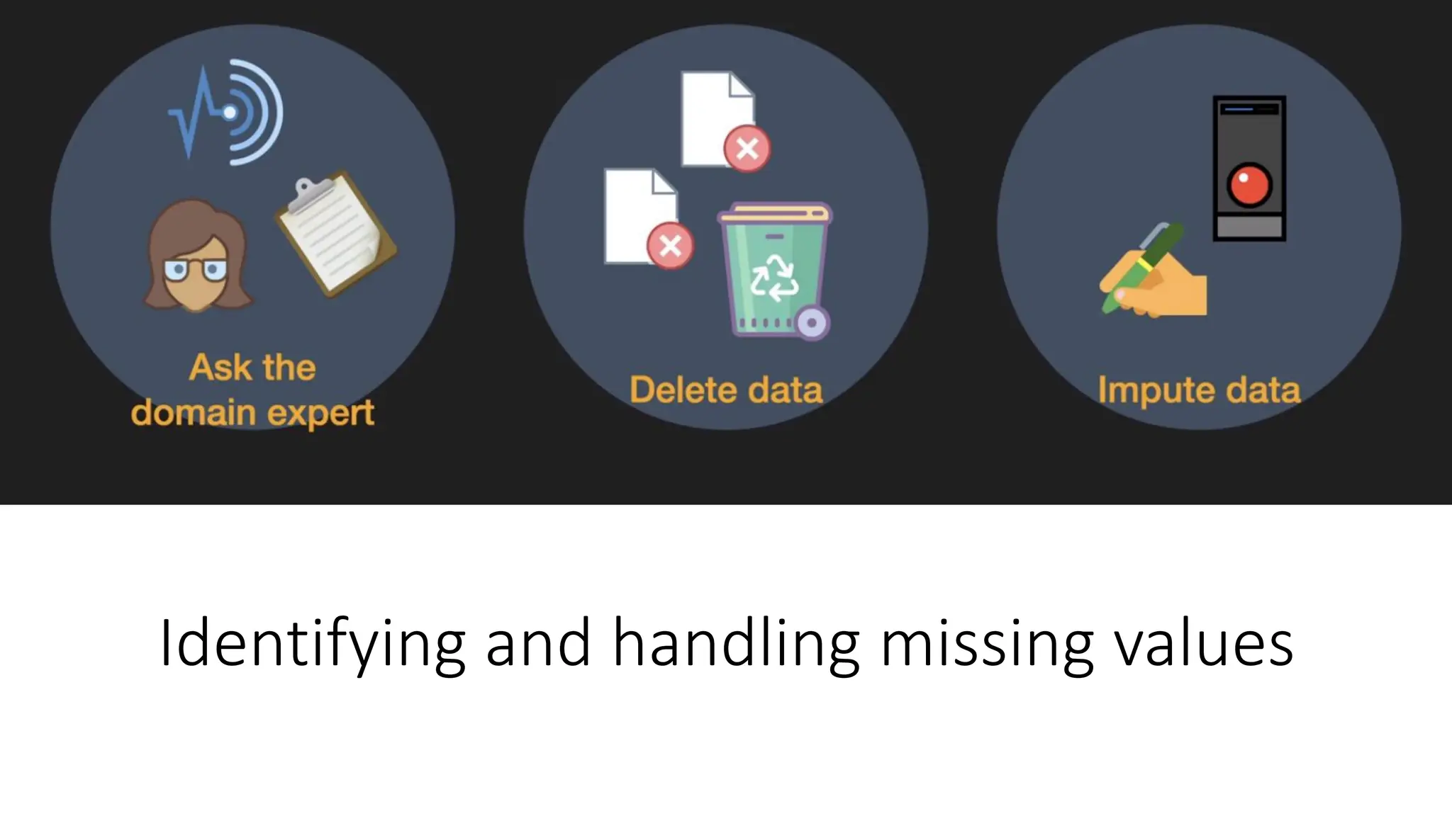
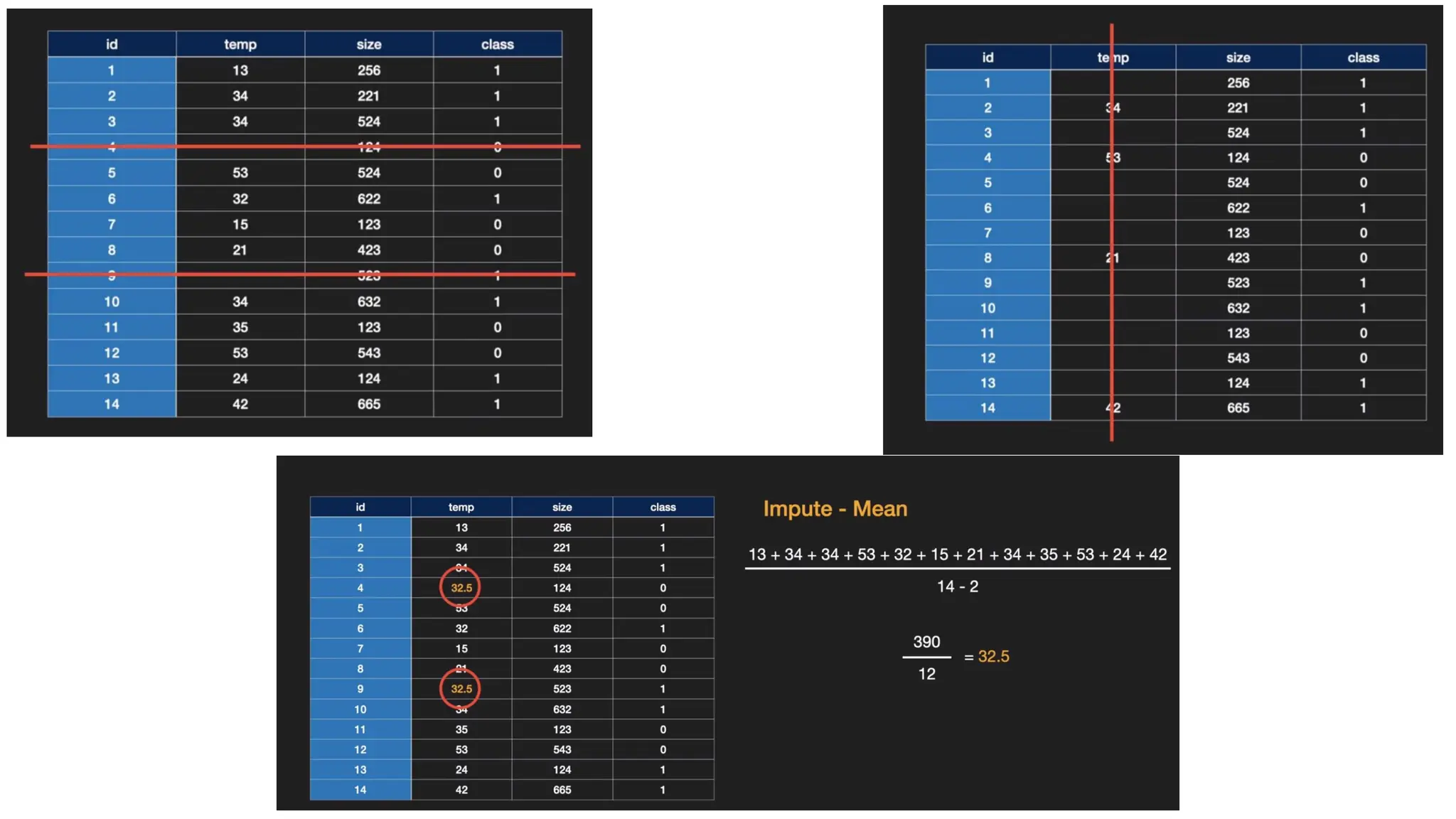
    Identifying and handlingmissing values • In data preprocessing, it is pivotal to identify and correctly handle the missing values, • Failing to handle missing values, you might draw inaccurate and faulty conclusions and inferences from the data. • There are two commonly used methods to handle missing data: (Ask the domain expert, which method to use) • Deleting a particular row • Impute the data • Replacing with the mean • Replacing with the median • Replacing with the most frequently occurring value • Replacing with a constant value
  • 28.
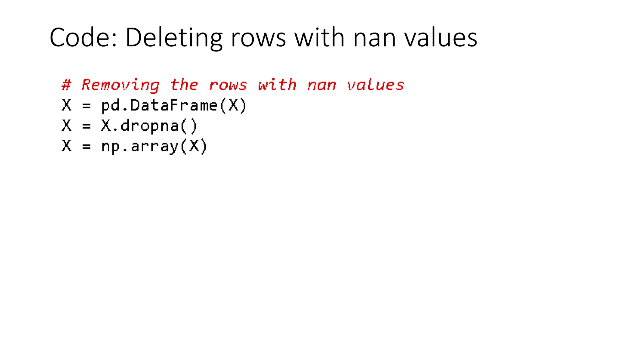
    Deleting a particularrow • You remove a specific row that has a null value for a feature or a particular column where more than 75% of the values are missing. • However, this method is not 100% efficient, and it is recommended that you use it only when the dataset has adequate samples. • You must ensure that after deleting the data, there remains no addition of bias.
  • 29.
    Code: Deleting rowswith nan values
  • 31.
    Impute data • Thismethod can add variance to the dataset, and any loss of data can be efficiently negated. • Hence, it yields better results compared to the first method (omission of rows/columns)
  • 32.
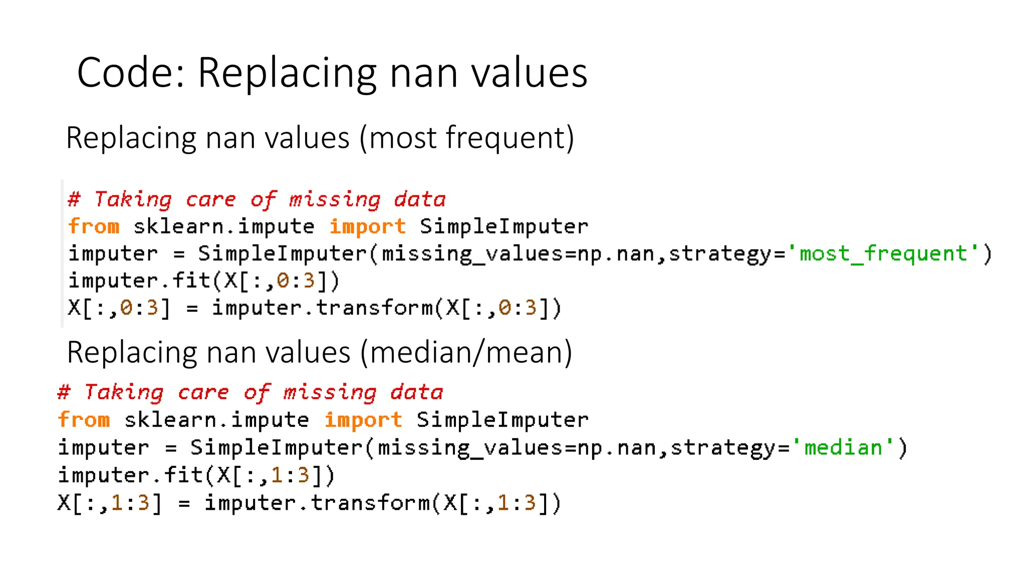
    Code: Replacing nanvalues Replacing nan values (most frequent) Replacing nan values (median/mean)
  • 33.
  • 34.
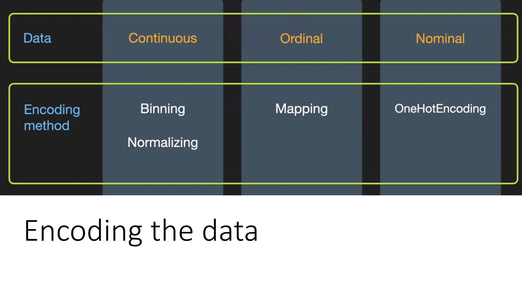
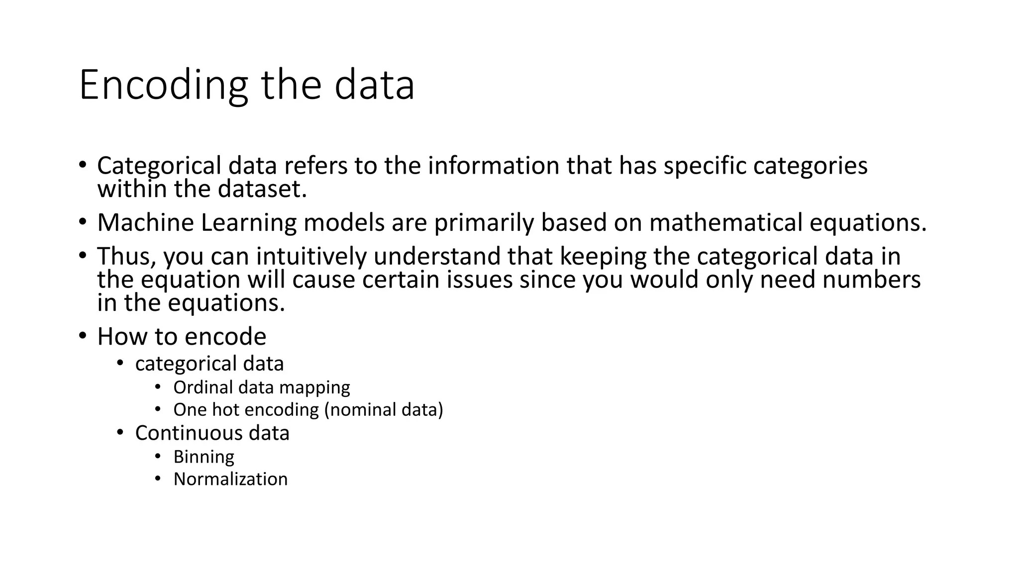
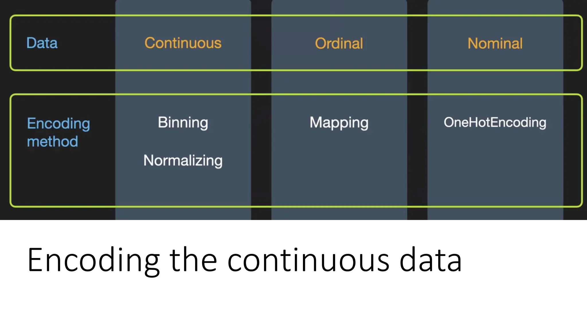
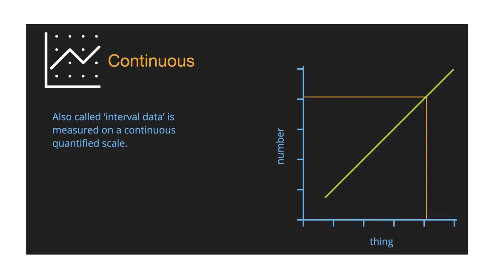
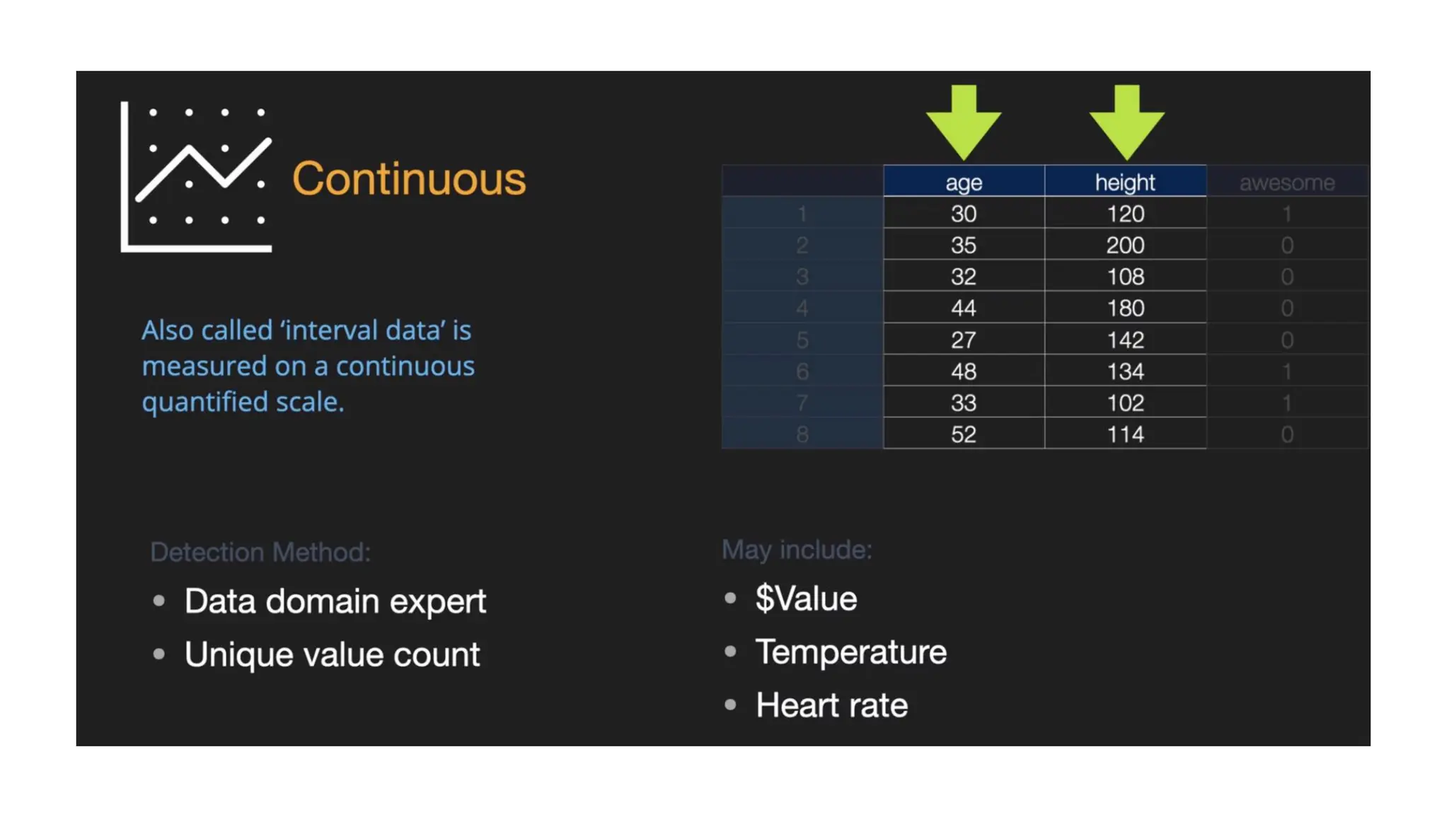
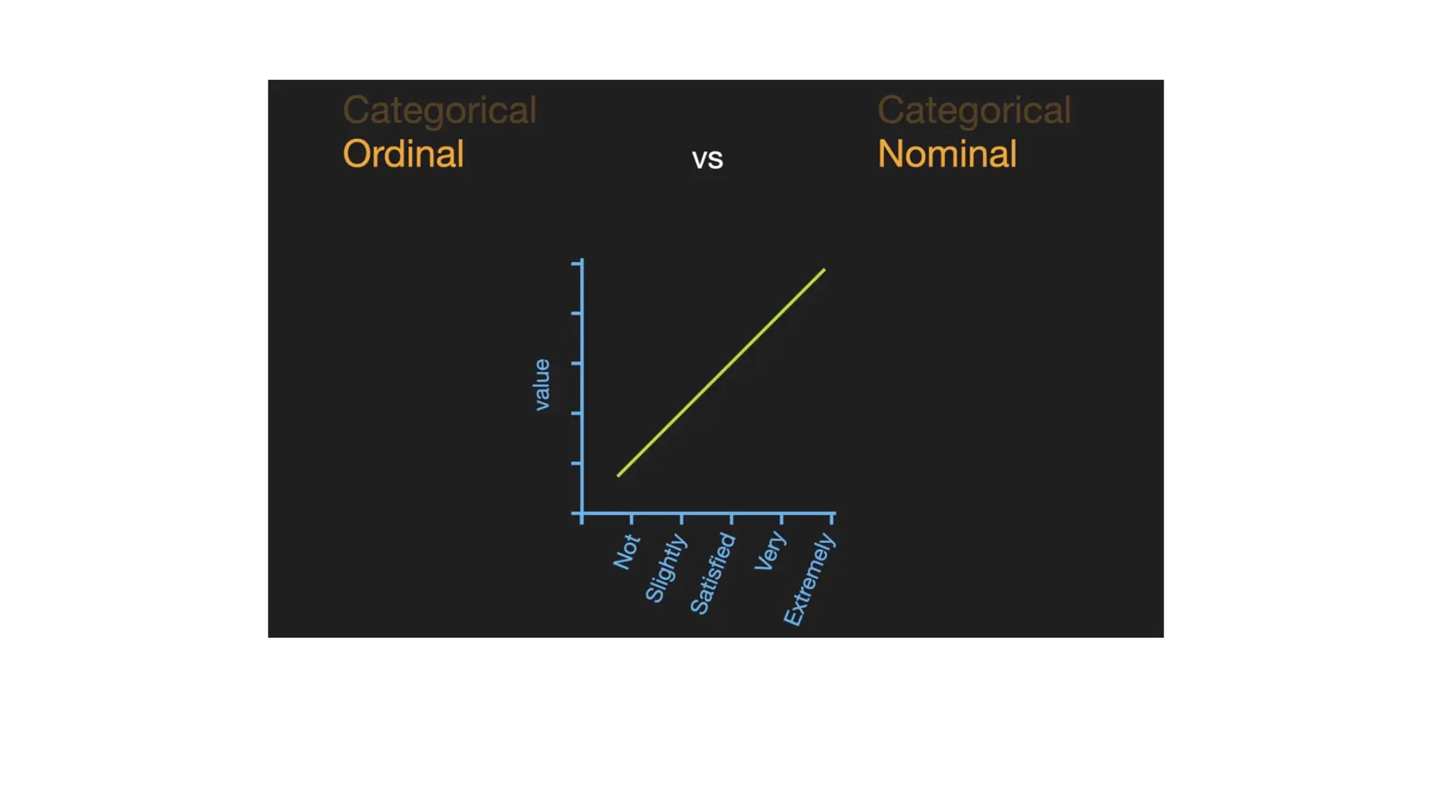
    Encoding the data •Categorical data refers to the information that has specific categories within the dataset. • Machine Learning models are primarily based on mathematical equations. • Thus, you can intuitively understand that keeping the categorical data in the equation will cause certain issues since you would only need numbers in the equations. • How to encode • categorical data • Ordinal data mapping • One hot encoding (nominal data) • Continuous data • Binning • Normalization
  • 35.
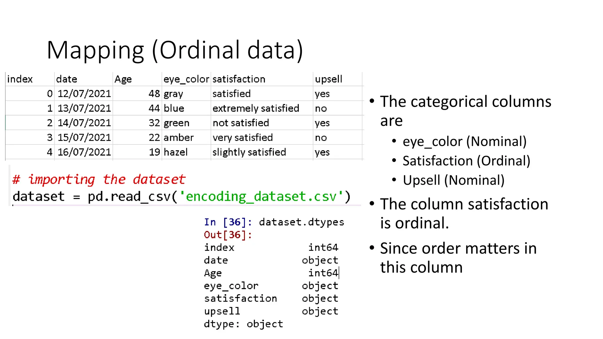
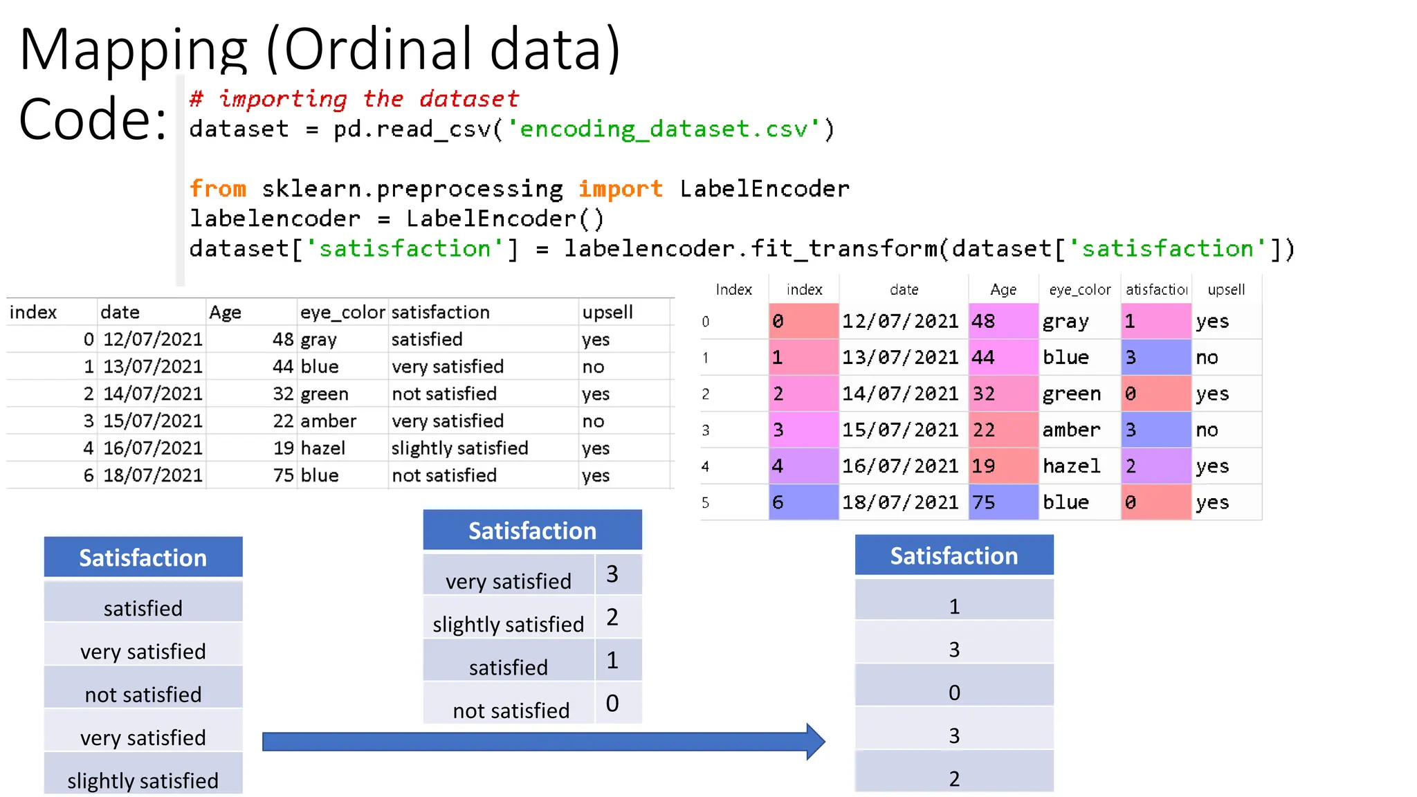
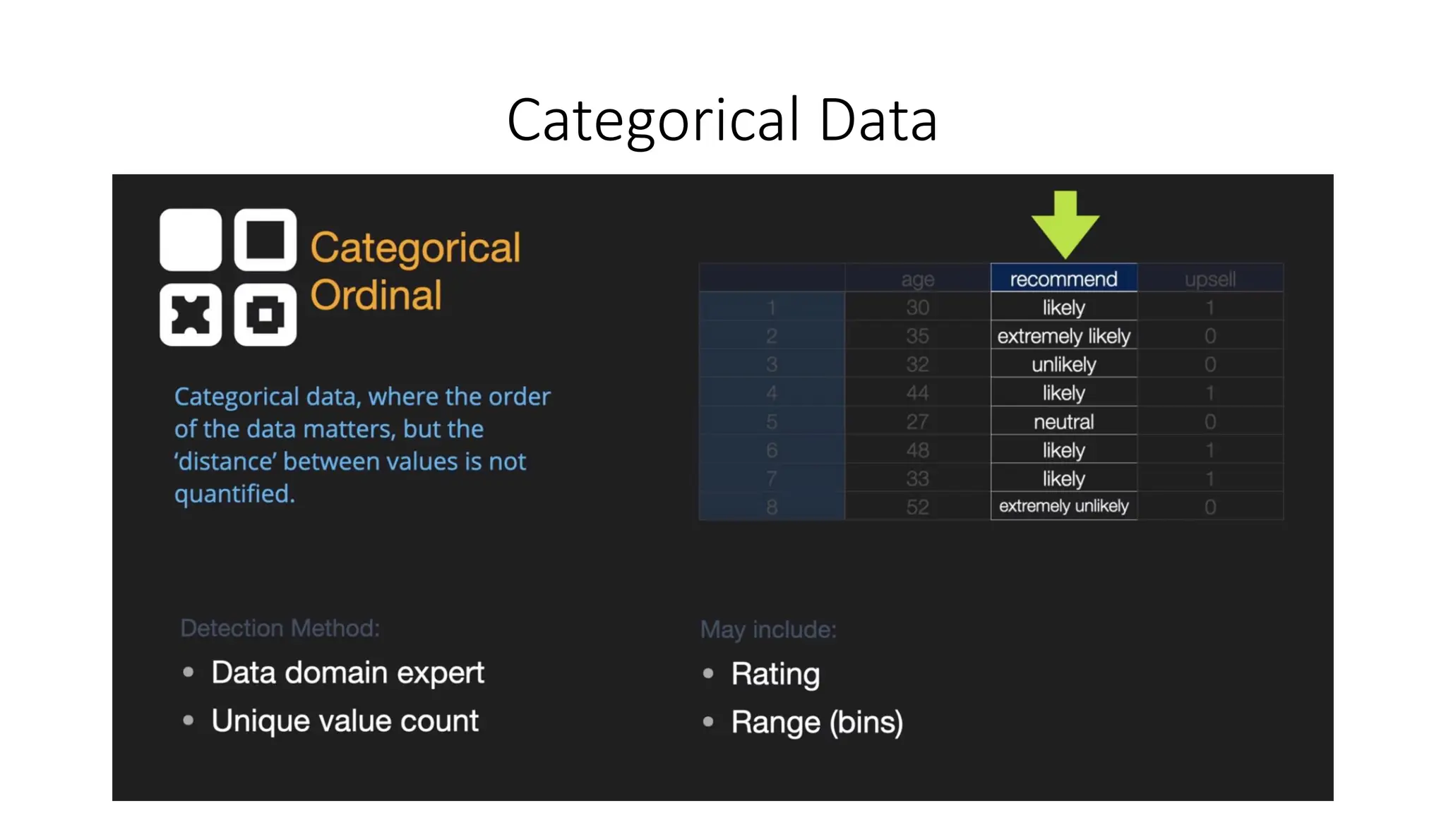
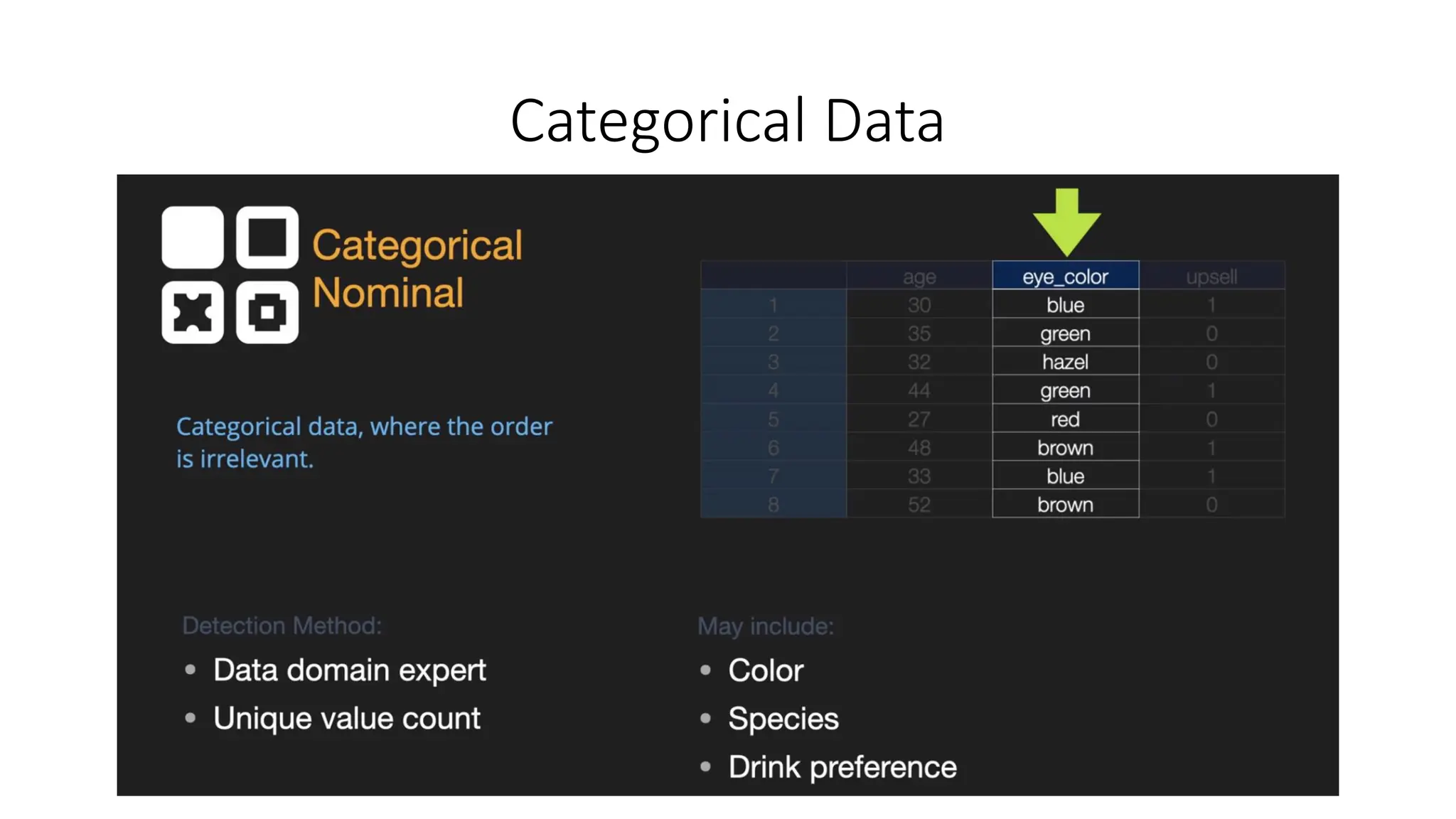
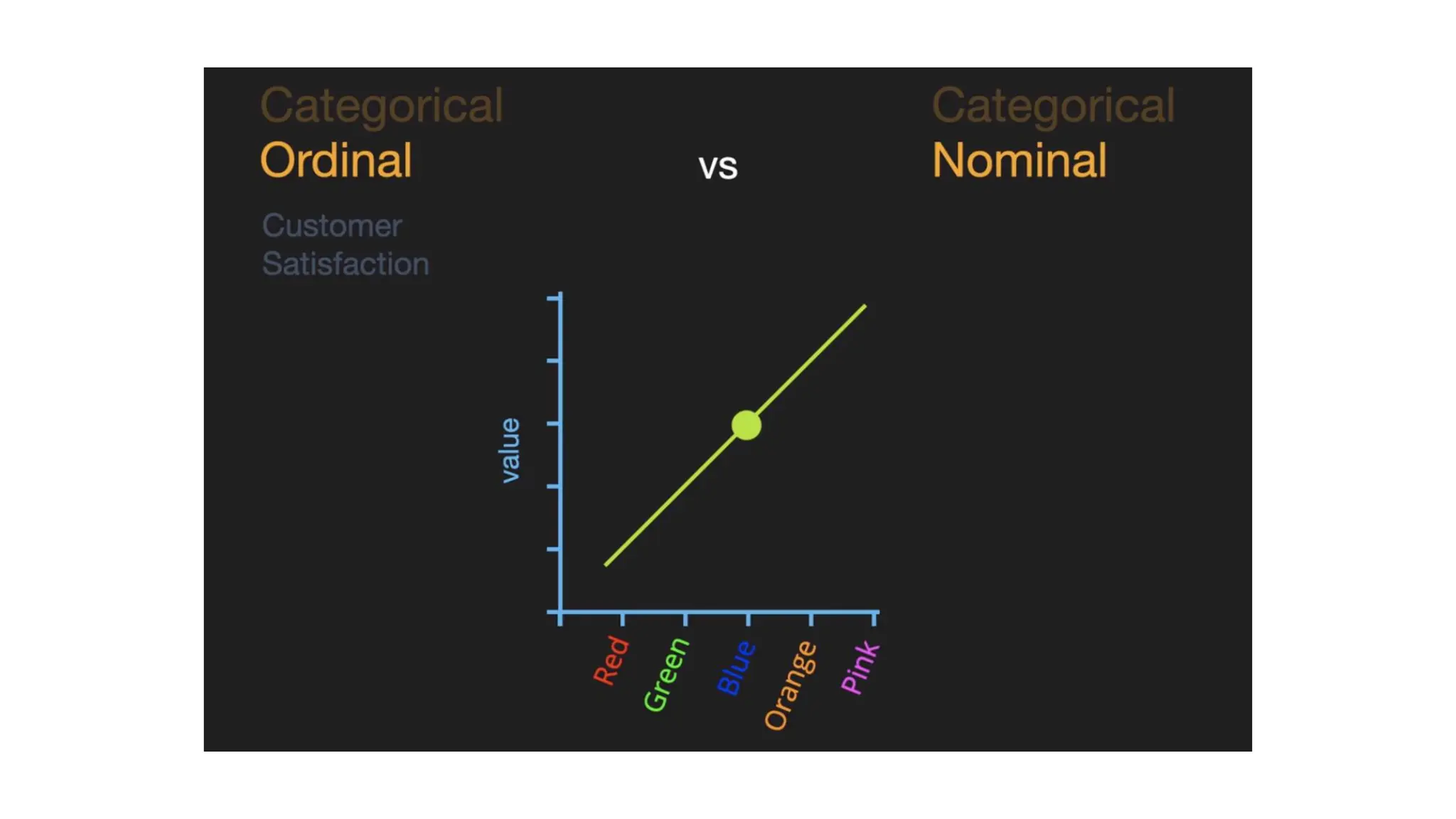
    Mapping (Ordinal data) •The categorical columns are • eye_color (Nominal) • Satisfaction (Ordinal) • Upsell (Nominal) • The column satisfaction is ordinal. • Since order matters in this column
  • 36.
    Mapping (Ordinal data) Code: Satisfaction satisfied verysatisfied not satisfied very satisfied slightly satisfied Satisfaction 1 3 0 3 2 Satisfaction very satisfied 3 slightly satisfied 2 satisfied 1 not satisfied 0
  • 37.
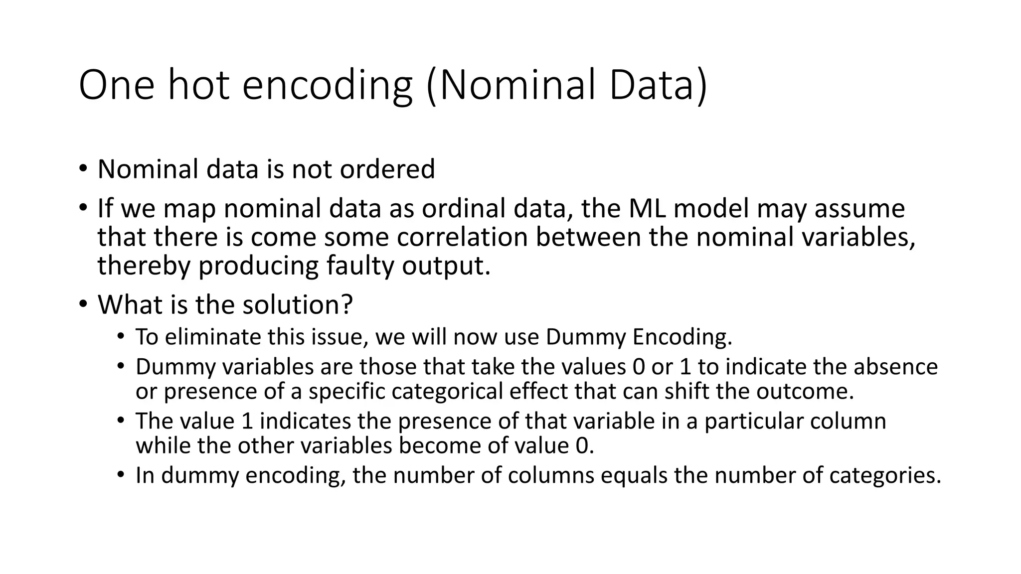
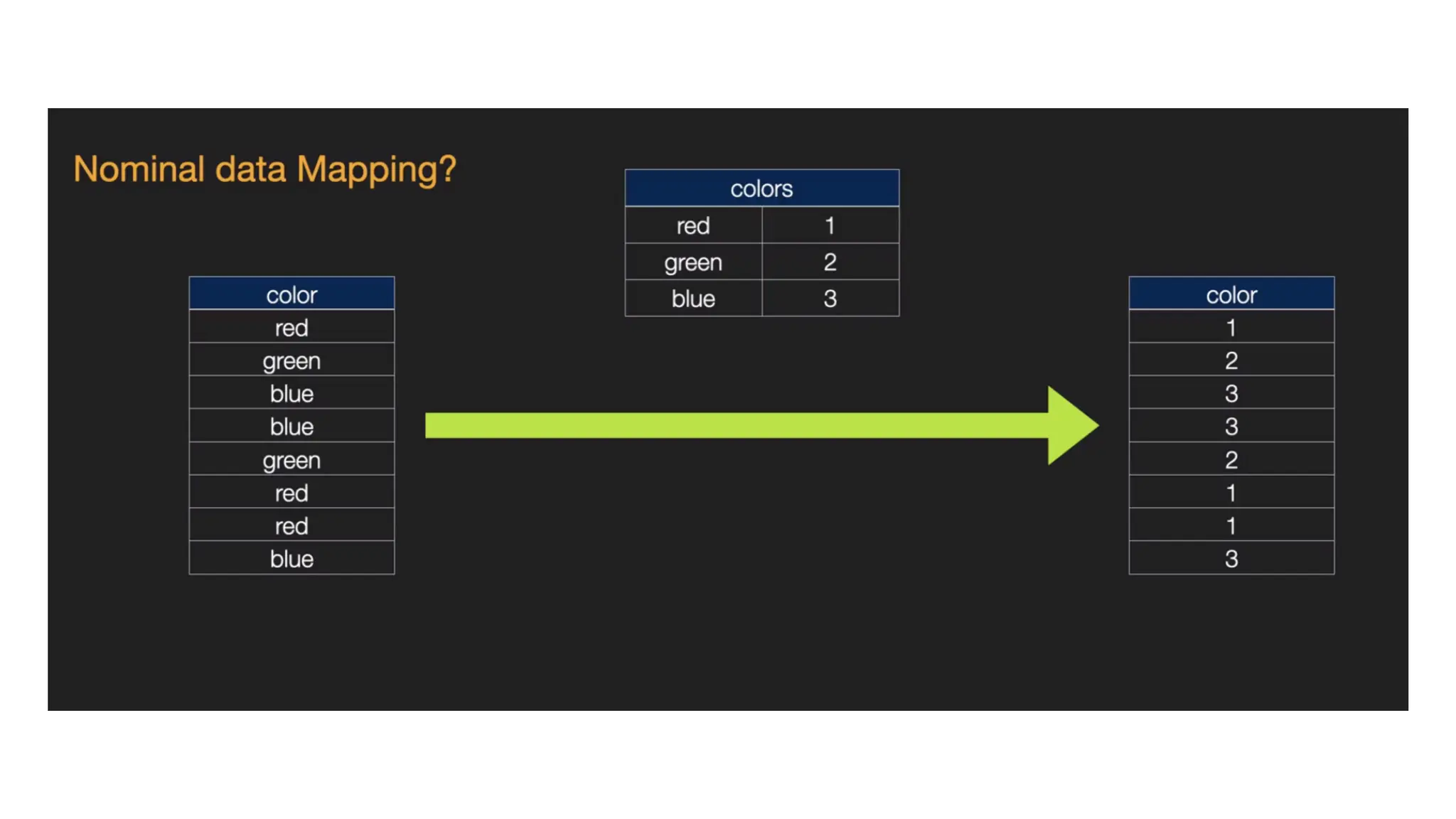
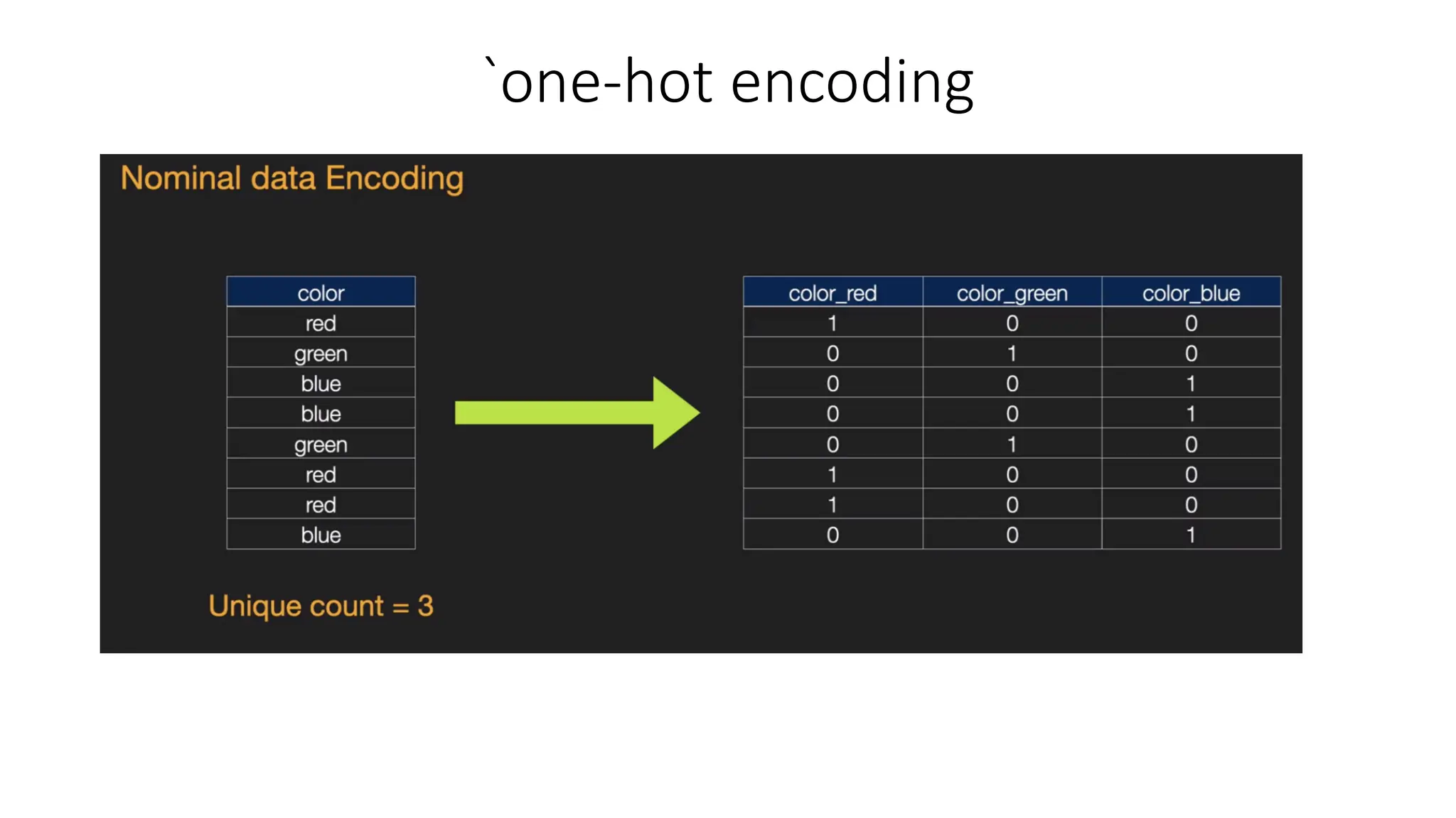
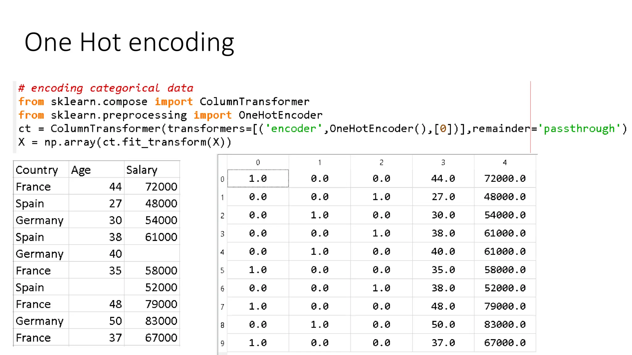
    One hot encoding(Nominal Data) • Nominal data is not ordered • If we map nominal data as ordinal data, the ML model may assume that there is come some correlation between the nominal variables, thereby producing faulty output. • What is the solution? • To eliminate this issue, we will now use Dummy Encoding. • Dummy variables are those that take the values 0 or 1 to indicate the absence or presence of a specific categorical effect that can shift the outcome. • The value 1 indicates the presence of that variable in a particular column while the other variables become of value 0. • In dummy encoding, the number of columns equals the number of categories.
  • 39.
  • 40.
  • 41.
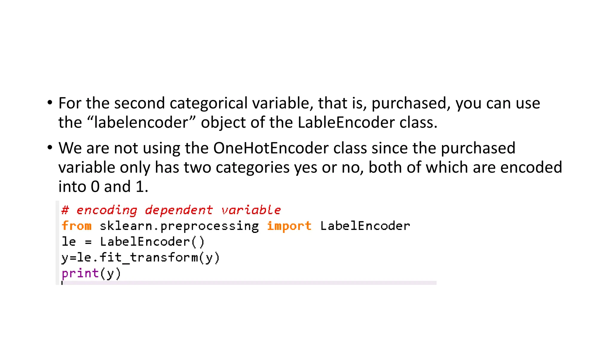
    • For thesecond categorical variable, that is, purchased, you can use the “labelencoder” object of the LableEncoder class. • We are not using the OneHotEncoder class since the purchased variable only has two categories yes or no, both of which are encoded into 0 and 1.
  • 42.
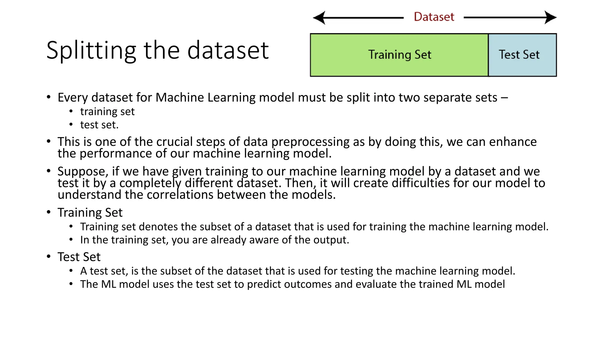
    Splitting the dataset •Every dataset for Machine Learning model must be split into two separate sets – • training set • test set. • This is one of the crucial steps of data preprocessing as by doing this, we can enhance the performance of our machine learning model. • Suppose, if we have given training to our machine learning model by a dataset and we test it by a completely different dataset. Then, it will create difficulties for our model to understand the correlations between the models. • Training Set • Training set denotes the subset of a dataset that is used for training the machine learning model. • In the training set, you are already aware of the output. • Test Set • A test set, is the subset of the dataset that is used for testing the machine learning model. • The ML model uses the test set to predict outcomes and evaluate the trained ML model
  • 43.
    • Usually, thedataset is split into 70:30 ratio or 80:20 ratio. • 70:30 ratio • This means that you take 70% of the data for training the model while leaving out the rest 30%. • 80:20 ratio • This means that you take 80% of the data for training the model while leaving out the rest 20%.
  • 44.
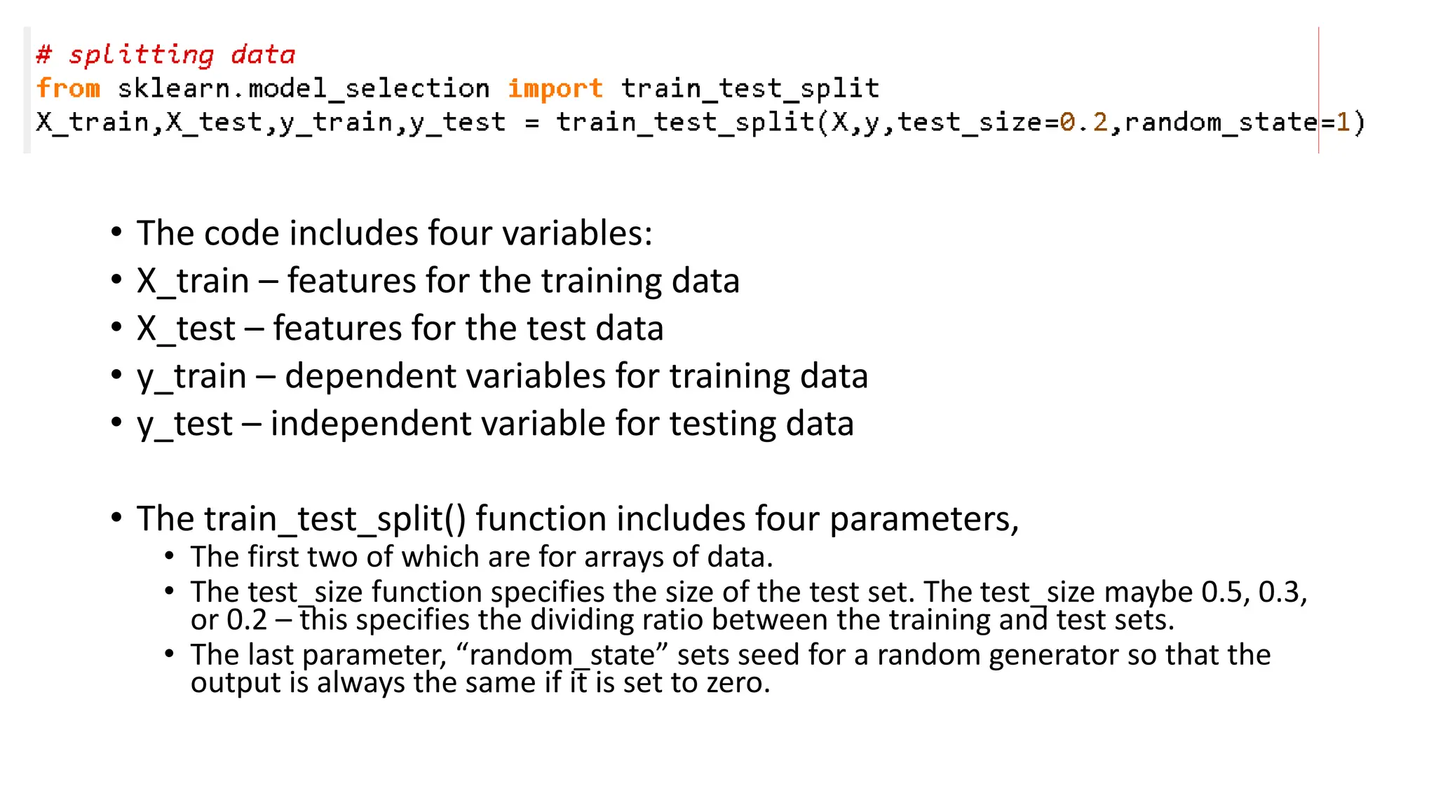
    • The codeincludes four variables: • X_train – features for the training data • X_test – features for the test data • y_train – dependent variables for training data • y_test – independent variable for testing data • The train_test_split() function includes four parameters, • The first two of which are for arrays of data. • The test_size function specifies the size of the test set. The test_size maybe 0.5, 0.3, or 0.2 – this specifies the dividing ratio between the training and test sets. • The last parameter, “random_state” sets seed for a random generator so that the output is always the same if it is set to zero.
  • 45.
  • 46.
    Feature Scaling (Normalization)and binning • Feature scaling and binning marks the end of the data preprocessing in Machine Learning. Feature Scaling • It is a method to standardize the independent variables of a dataset within a specific range. • In other words, feature scaling limits the range of variables so that you can compare them on common grounds. • It prevents algorithms from being influenced by higher values
  • 49.
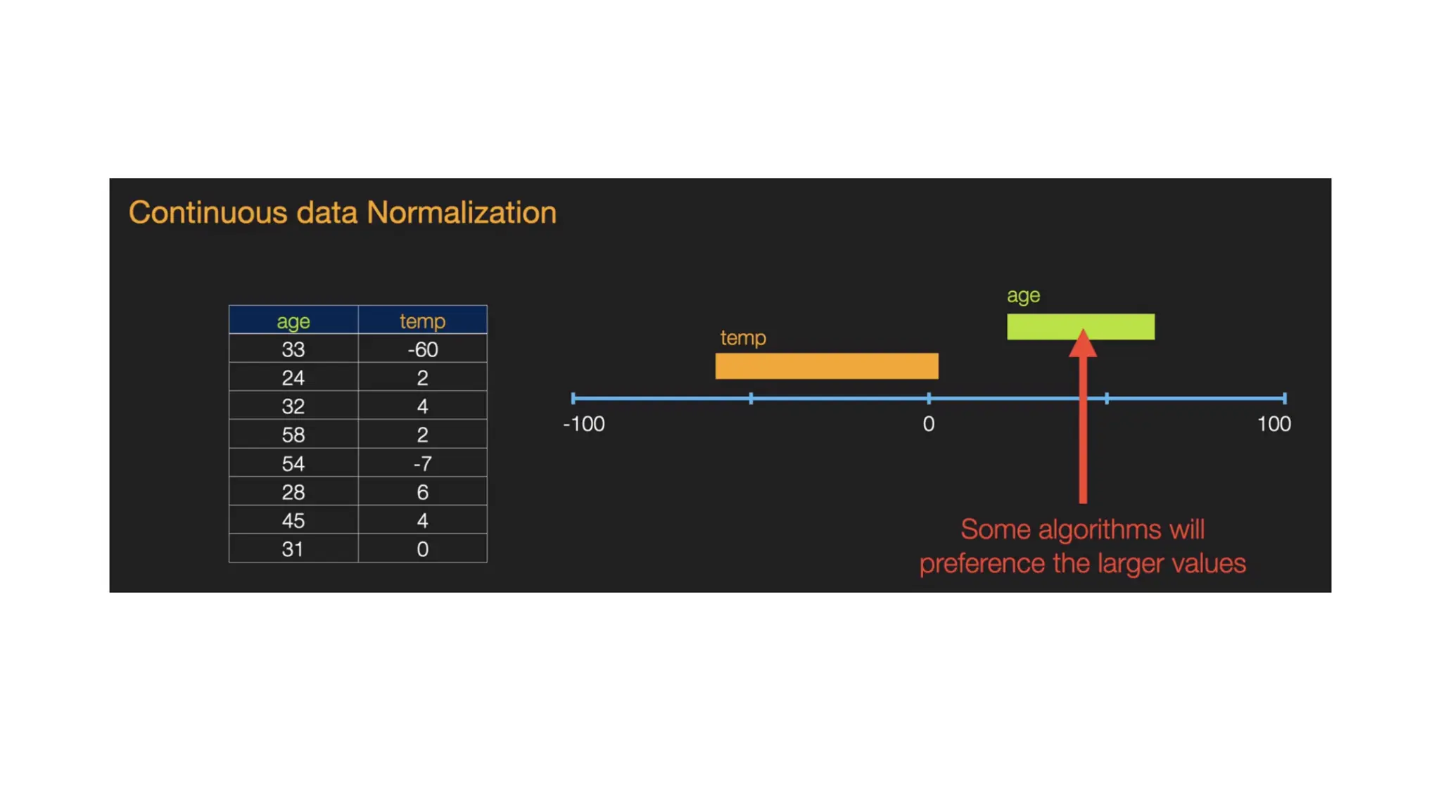
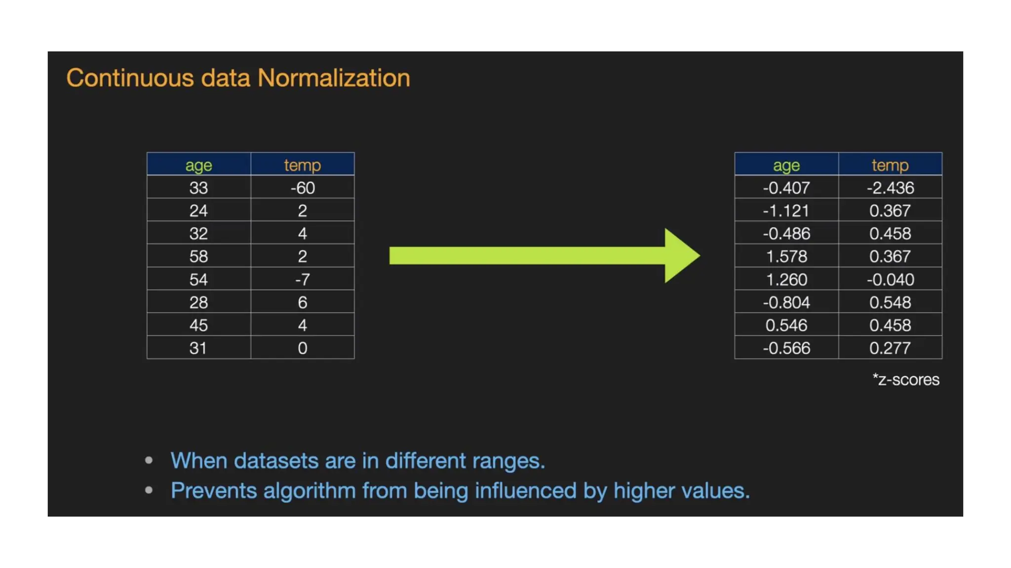
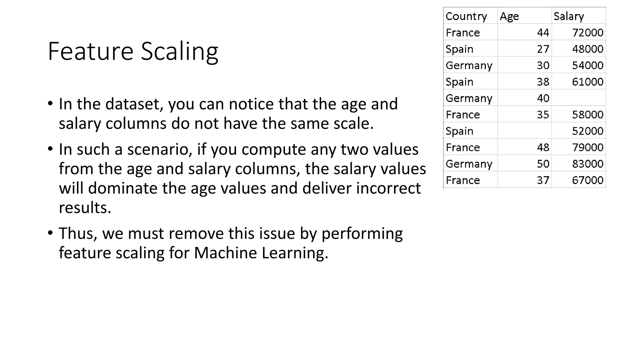
    Feature Scaling • Inthe dataset, you can notice that the age and salary columns do not have the same scale. • In such a scenario, if you compute any two values from the age and salary columns, the salary values will dominate the age values and deliver incorrect results. • Thus, we must remove this issue by performing feature scaling for Machine Learning.
  • 50.
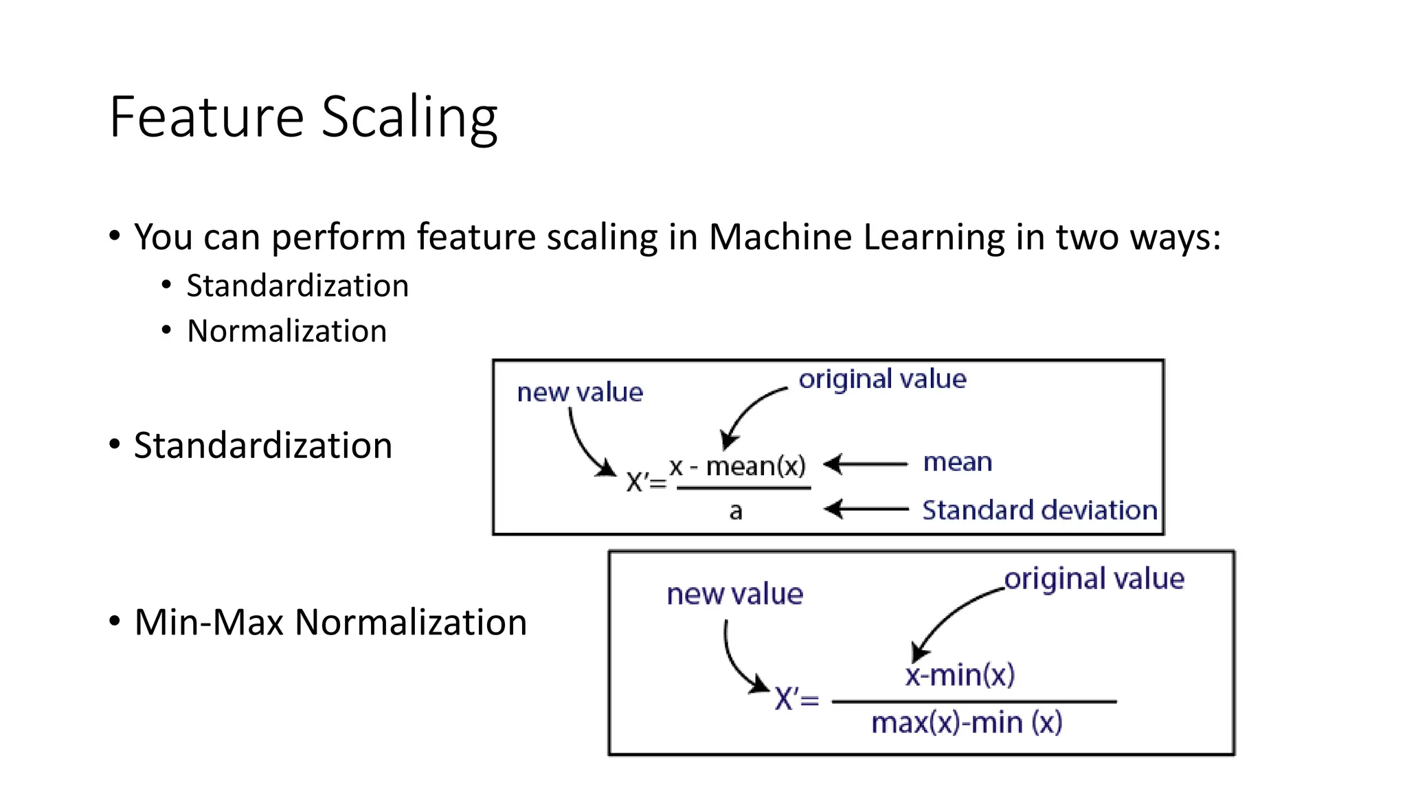
    Feature Scaling • Youcan perform feature scaling in Machine Learning in two ways: • Standardization • Normalization • Standardization • Min-Max Normalization
  • 51.
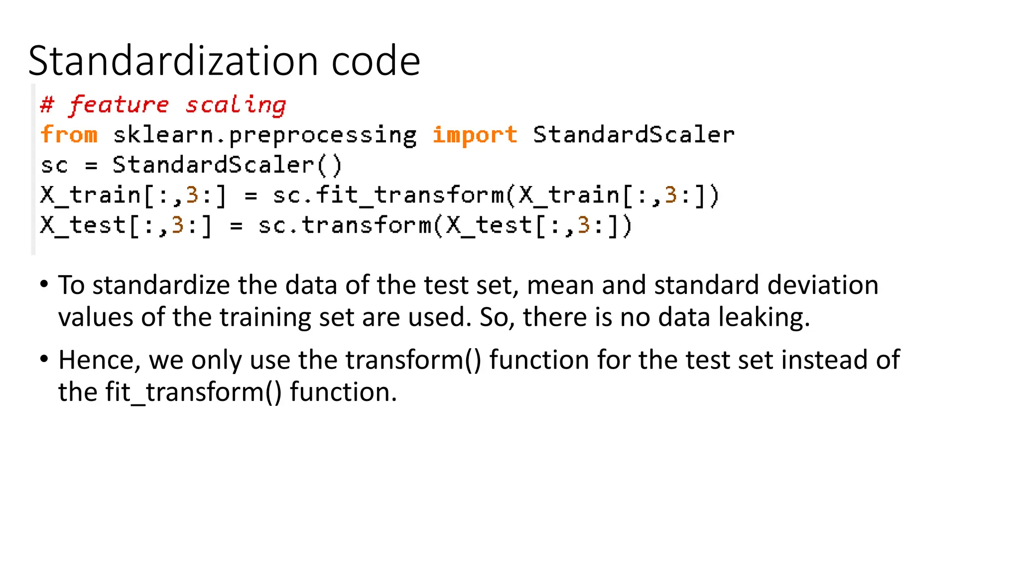
    Standardization code • Tostandardize the data of the test set, mean and standard deviation values of the training set are used. So, there is no data leaking. • Hence, we only use the transform() function for the test set instead of the fit_transform() function.
  • 52.
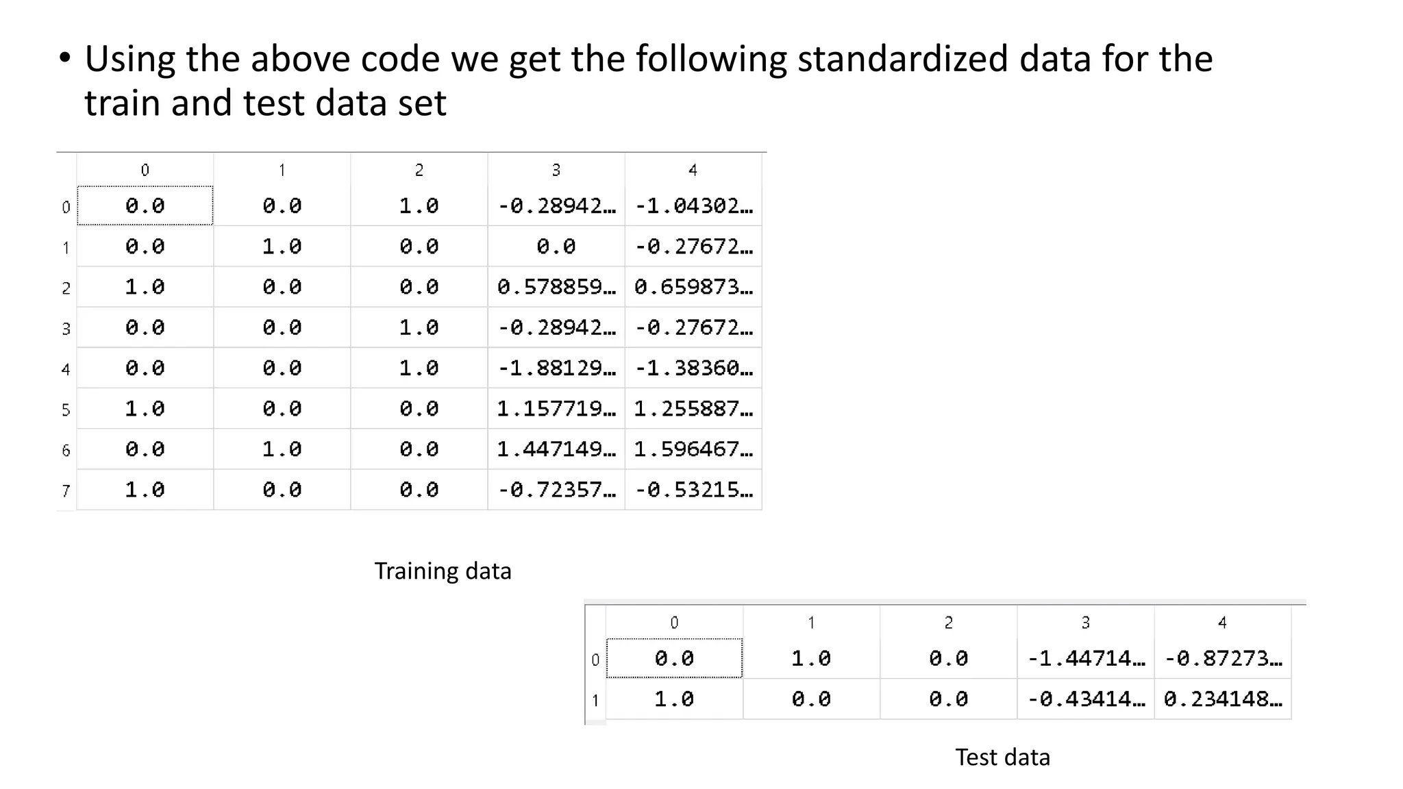
    • Using theabove code we get the following standardized data for the train and test data set Training data Test data
  • 53.
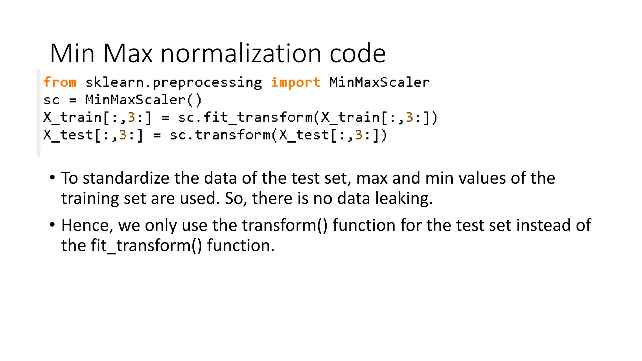
    Min Max normalizationcode • To standardize the data of the test set, max and min values of the training set are used. So, there is no data leaking. • Hence, we only use the transform() function for the test set instead of the fit_transform() function.
  • 54.
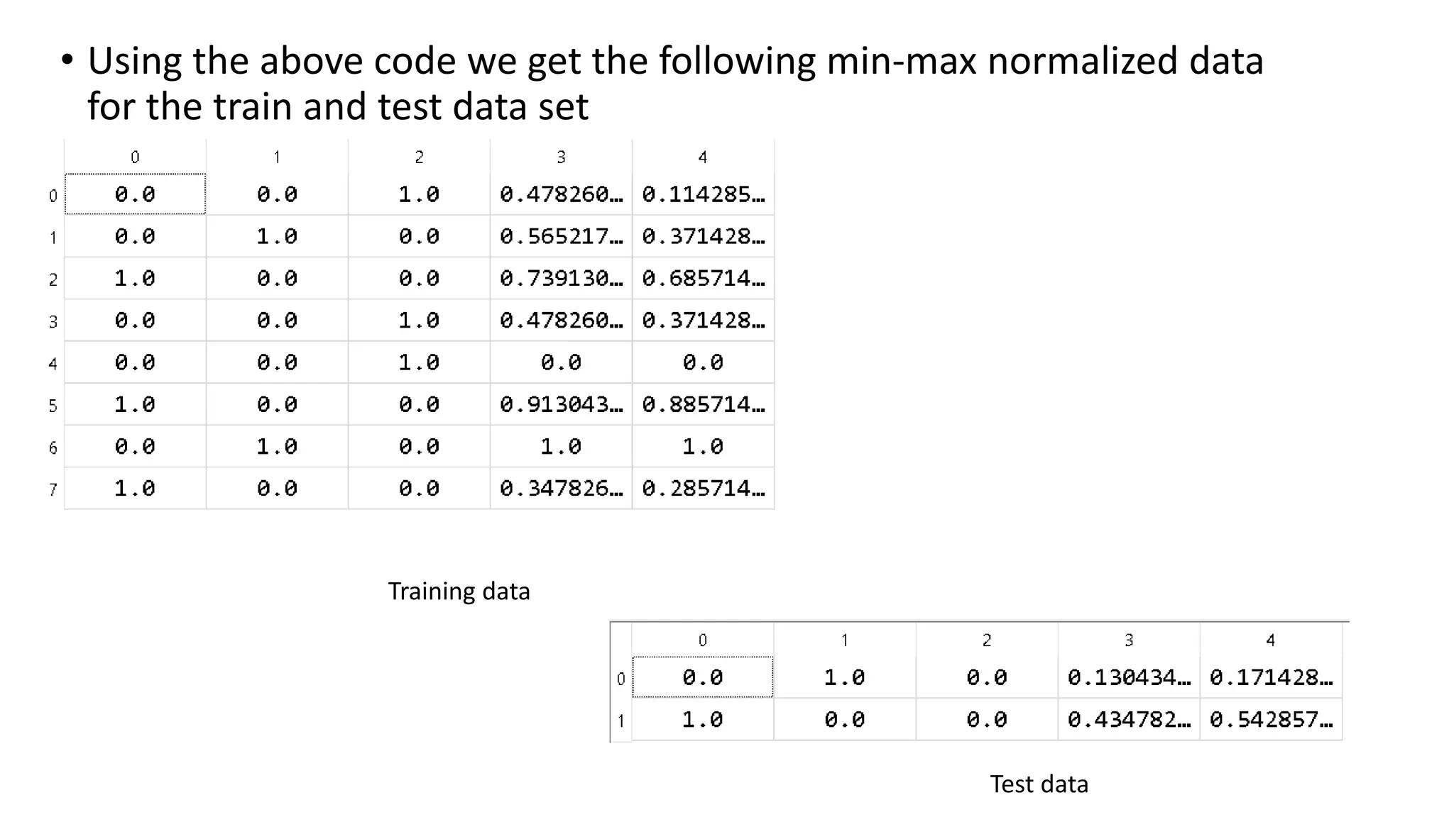
    • Using theabove code we get the following min-max normalized data for the train and test data set Training data Test data
  • 55.
  • 58.
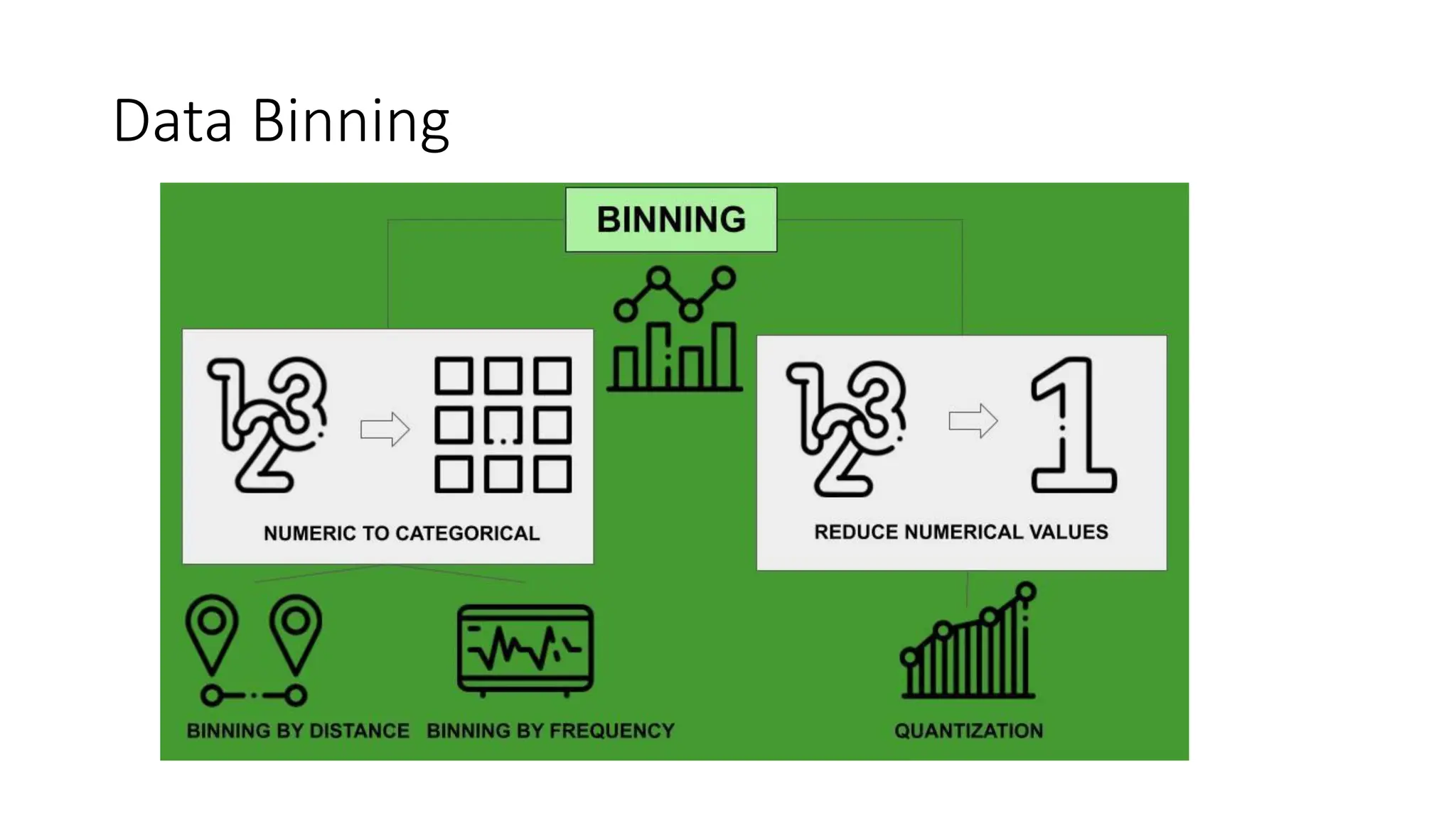
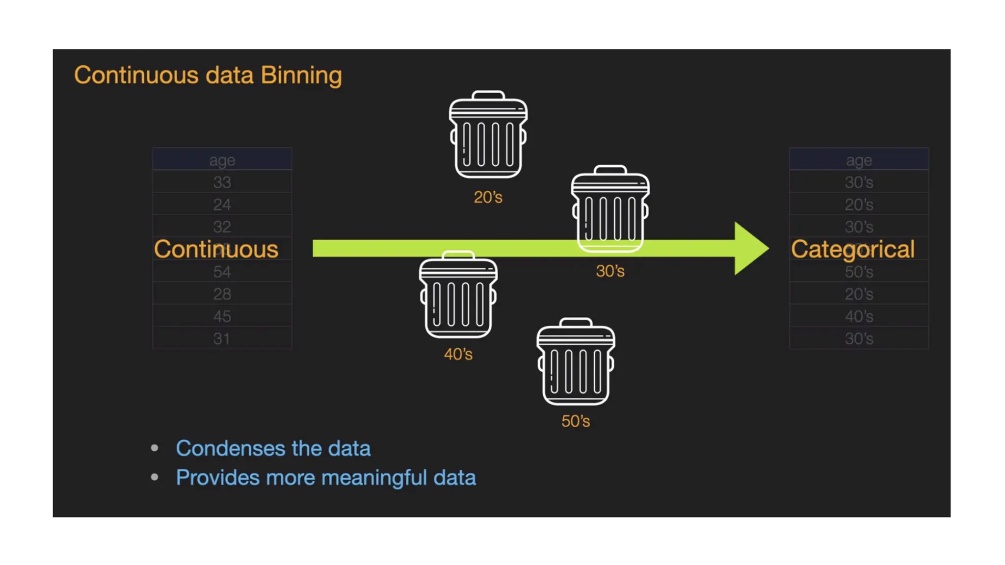
    • Data binning/bucketinggroups data in bins/buckets, in the sense that it replaces values contained into a small interval with a single representative value for that interval. • Sometimes binning improves accuracy in predictive models. • Binning can be applied to • convert numeric values to categorical values • binning by distance • binning by frequency • Reduce numeric values • quantization (or sampling)
  • 59.
    • Binning isa technique for data smoothing. • Data smoothing is employed to remove noise from data. • Three techniques are used for data smoothing: • binning • regression • outlier analysis • We will cover only binning here
  • 60.
    Example: cupcake • Googletrends • Shows the search trends of cupcakes in the world. • Code:
  • 61.
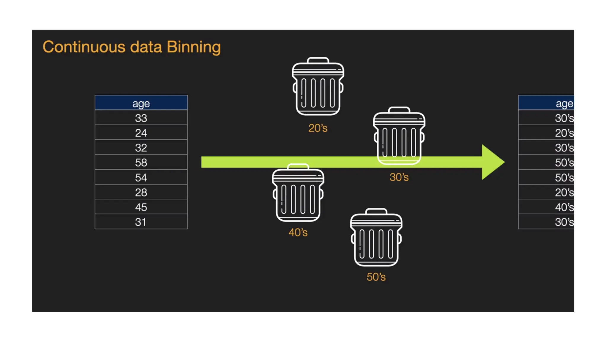
    Binning by distance •Import the dataset • Compute the range of values and find the edges of intervals/bins • Define labels • convert numeric values into categorical labels • Plot the histogram to see the distribution
  • 62.
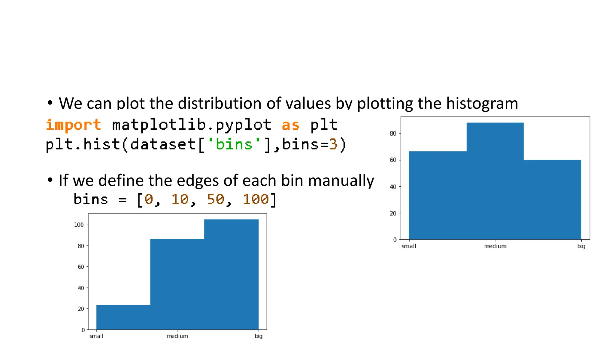
    Binning by distance •In this case we define the edges of each bin • We group values related to the column into • Small • Medium • Big • We need to calculate the intervals within which each group falls. • We calculate the interval range as the difference between the maximum and minimum value and then we split this interval into “N=3” parts, one for each group.
  • 63.
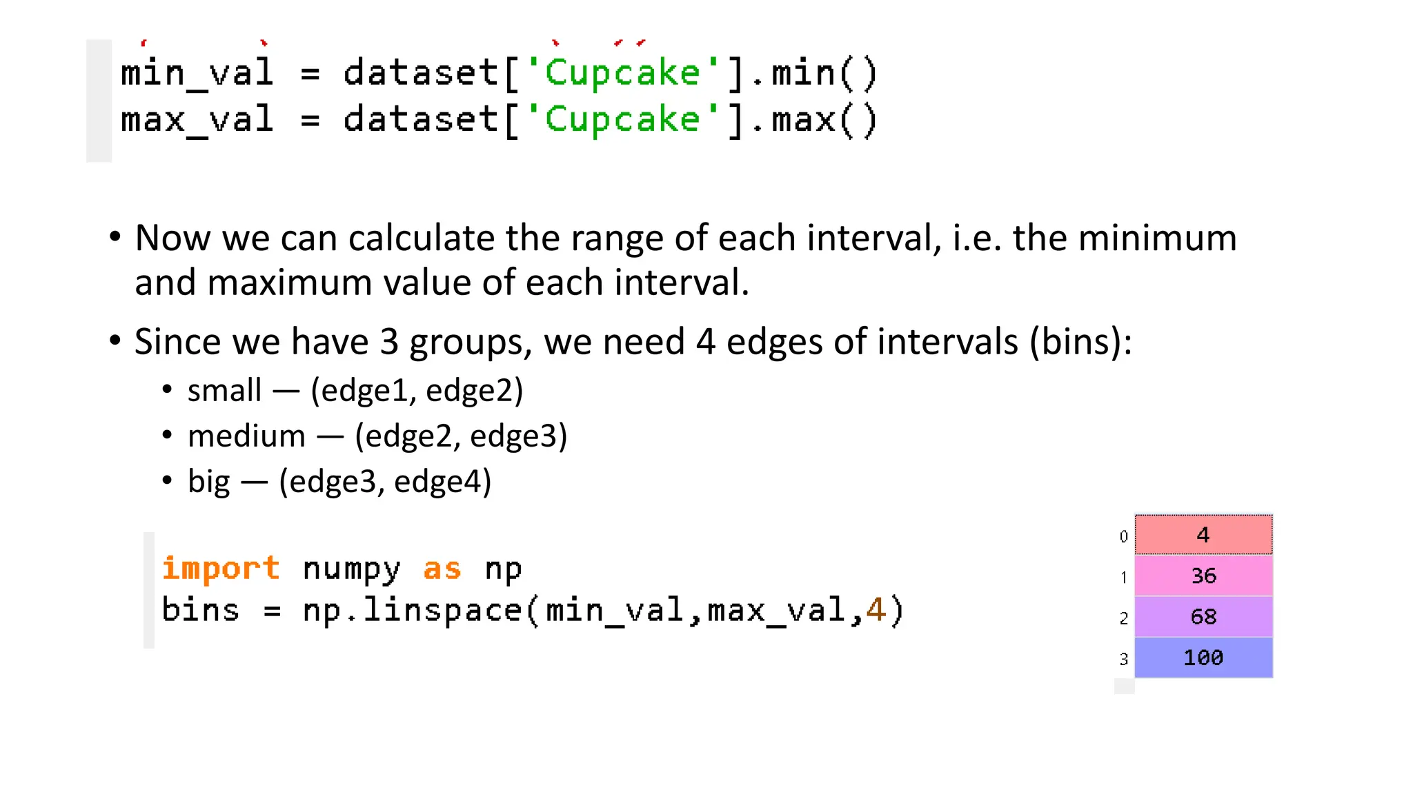
    • Now wecan calculate the range of each interval, i.e. the minimum and maximum value of each interval. • Since we have 3 groups, we need 4 edges of intervals (bins): • small — (edge1, edge2) • medium — (edge2, edge3) • big — (edge3, edge4)
  • 64.
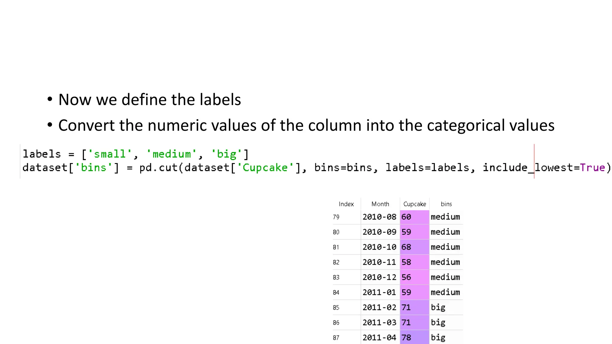
    • Now wedefine the labels • Convert the numeric values of the column into the categorical values
  • 65.
    • We canplot the distribution of values by plotting the histogram • If we define the edges of each bin manually
  • 66.
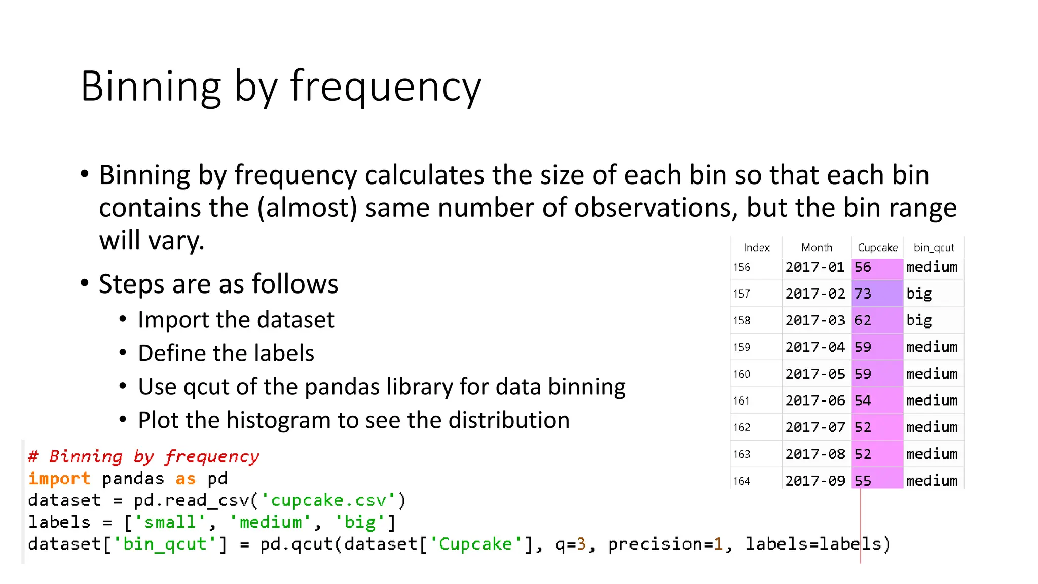
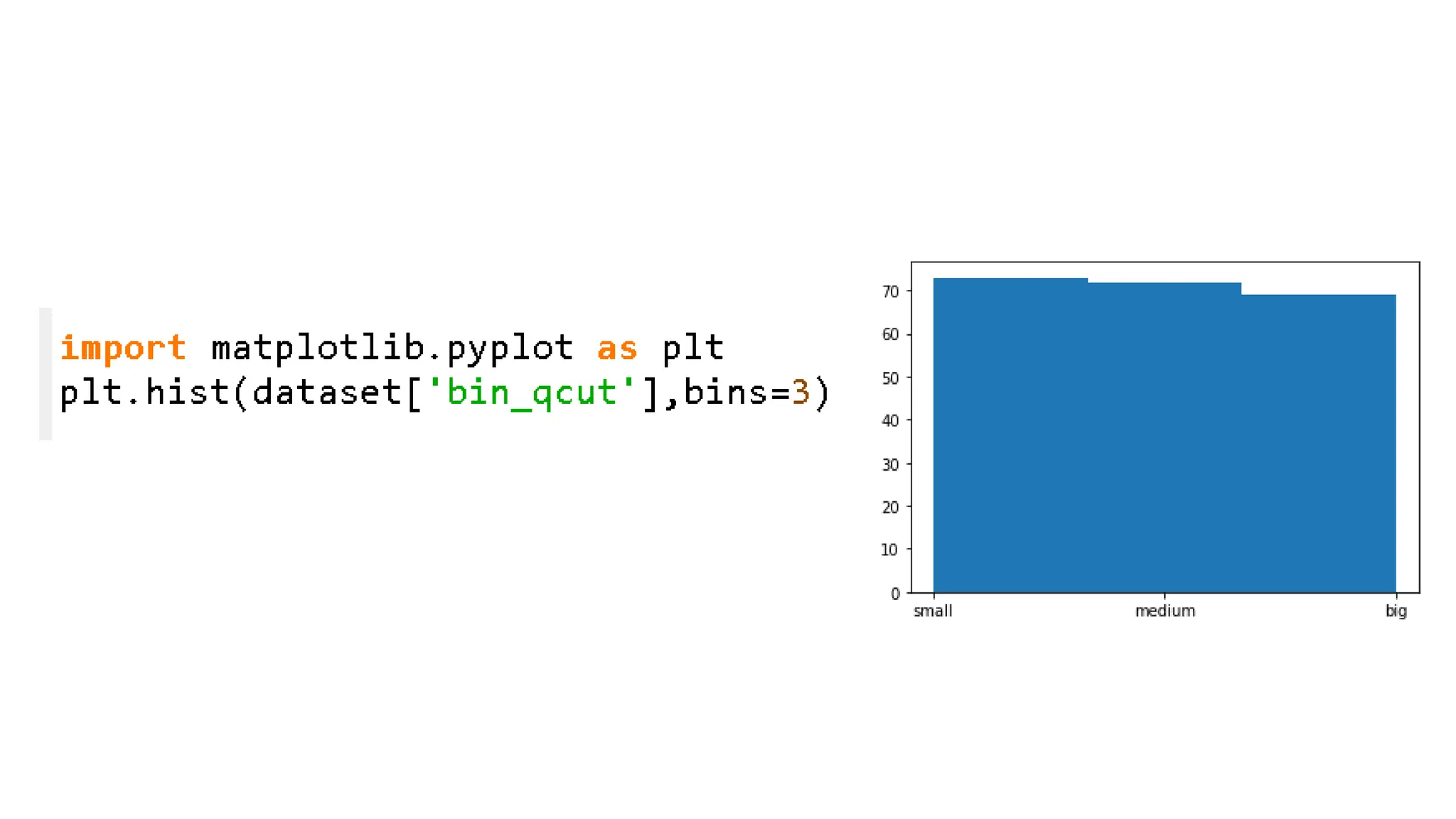
    Binning by frequency •Binning by frequency calculates the size of each bin so that each bin contains the (almost) same number of observations, but the bin range will vary. • Steps are as follows • Import the dataset • Define the labels • Use qcut of the pandas library for data binning • Plot the histogram to see the distribution
  • 68.
    Binning by Sampling •Sampling is another technique of data binning. • It permits to reduce the number of samples, by grouping similar values or contiguous values. • There are three approaches to perform sampling: • binning by mean: • Each value in a bin is replaced by the mean value of the bin. • Binning by median: • Each bin value is replaced by its bin median value. • Binning by boundary: • each bin value is replaced by the closest boundary value, i.e. maximum or minimum value of the bin.
  • 69.
    Binning by mean •Import the dataset • Compute the range of each bin and compute the mean of each bin • Compute the bin edges of each bin • Set the value of each bin to the mean value • Plot the distribution
  • 70.
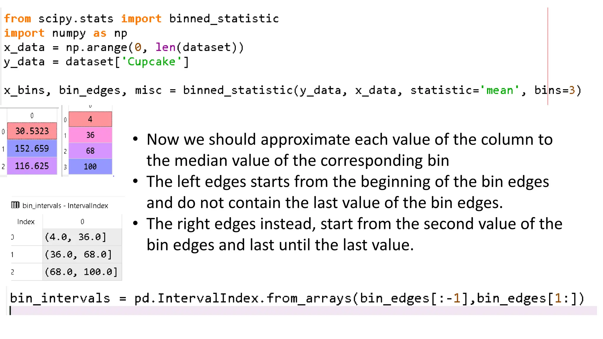
    • Now weshould approximate each value of the column to the median value of the corresponding bin • The left edges starts from the beginning of the bin edges and do not contain the last value of the bin edges. • The right edges instead, start from the second value of the bin edges and last until the last value.
  • 71.
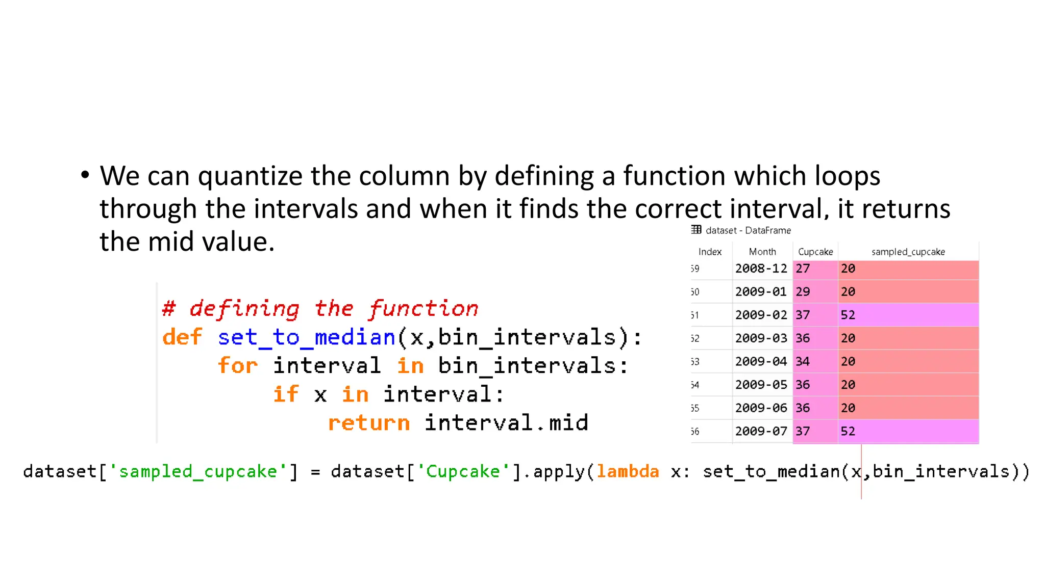
    • We canquantize the column by defining a function which loops through the intervals and when it finds the correct interval, it returns the mid value.
  • 80.
  • 86.
  • 87.