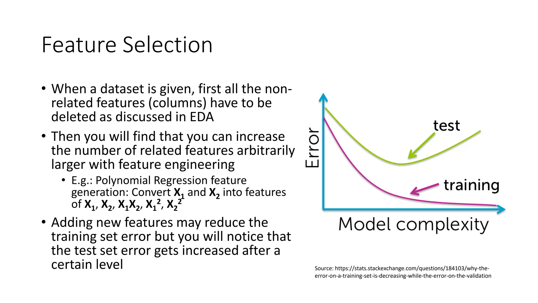
DA 5230 – Statistical & Machine Learning Lecture 8 – Feature Engineering and Optimization Maninda Edirisooriya manindaw@uom.lk
Features • In general Features are X values/Independent Variables or Predictor Variables of a Dataset • Features can be • Numerical values • Categorical labels • Complex structures like texts or images • Having high quality (with more and relevant information) and independent (with information not shared with other features) features can improve model accuracy • Having lower quality and highly correlated (less independent) features can reduce model accuracy (due to noise) and increase computational burden
Feature Selection • When a dataset is given, first all the non- related features (columns) have to be deleted as discussed in EDA • Then you will find that you can increase the number of related features arbitrarily larger with feature engineering • E.g.: Polynomial Regression feature generation: Convert X1 and X2 into features of X1, X2, X1X2, X1 2, X2 2 • Adding new features may reduce the training set error but you will notice that the test set error gets increased after a certain level Source: https://stats.stackexchange.com/questions/184103/why-the- error-on-a-training-set-is-decreasing-while-the-error-on-the-validation
Feature Selection • Therefore, you have to find the optimum features that minimizes the test set error • This process is known as Feature Selection • When there are n number of candidate features there are 𝒏! 𝒓! 𝒏−𝒓 ! different ways of selecting r number of features • As the optimum r can be any number, the search space for all possible r becomes ෍ 𝒓=𝟏 𝒏 𝒏! 𝒓! 𝒏−𝒓 ! which grows exponentially with n • This is known as the Curse of Dimensionality • Forward Selection or Backward Elimination algorithm can be used to select features without this exponential search space growth
Forward Selection • In Forward Selection, we start with an empty set of features • In each iteration we add the best feature to the model feature set so that the model performance is increased in the test set • Here the model performance increase in the test set is used as the evaluation criteria of the algorithm • If all the features are added OR if there is no new feature remaining that increases the model performance when added, stop the algorithm • This is the stopping criteria of the algorithm
Backward Elimination • In Backward Elimination we start with all the available features • In each iteration we remove the worst feature from the model feature set so that the model performance is increased in the test set • Here the model performance increase in the test set is used as the evaluation criteria of the algorithm • If all the features are removed OR if there is no existing feature remaining that increases the model performance when removed, stop the algorithm • This is the stopping criteria of the algorithm
Common Nature of these Algorithms • These algorithms are faster than the pure Feature Selection • In these algorithms, the evaluation criteria and stopping criteria can be customized as you like • E.g.: Maximum/minimum number of features can also be used as the stopping criteria as well • Cross-validation performance increase can be used as the evaluation criteria when the dataset is small • Because these are heuristic algorithms, we may miss some better feature combinations which may result better performance • That is what we sacrifice for the speed of these new algorithms
Feature Transformation Numerical features may exist with unwanted distributions For example, some X values in a dataset for a Linear Regression can be non- linear which can be transformed to a linear relationship using a higher degree of that variable X1 Y Y X1 2 Transformation X1 → X1 2 or X1 → exp(X1)
Feature Transformation Non-normal frequency distributions can be converted to normal distributions like follows X1 X1 2 n’th root OR log(X1) Right skewed Distribution Normal Distribution X1 Frequency X1 2 n’th power OR exp(X1) Left skewed Distribution Normal Distribution Frequency Frequency Frequency
Feature Encoding • Many machine learning algorithms need numerical values for their X variables • Therefore categorical variables have to be converted into numerical variables, to be used them as model features • There are many ways to encode categorical variables to numerical • Nominal variables (e.g.: Color, Gender) are generally encoded with One-Hot Encoding • Ordinal variables (e.g.: T-shirt size, Age group) are generally encoded with Label Encoding
One-Hot Encoding Encode Outlet Size Source: https://www.youtube.com/watch?v=uu8um0JmYA8
Label Encoding Encode Outlet Size Source: https://www.youtube.com/watch?v=uu8um0JmYA8
Scaling Features • Numerical data features of a dataset can have different scales • E.g.: Number of bedrooms in a house may spread between 1 to 5 while the square feet of a house can spread between 500 to 4000 • When these features are used as they are, there can be problems when taking vector distances between each other • E.g.: Can affect the convergence rate in Gradient Descent algorithm • When regularization is applied, most L1 and L2 regularization components are applied in the same scale for all the features • i.e.: Small scale features are highly regularized and vice versa • Interpreting a model can be difficult, as model parameter scales can be affected by the feature’s scale
Scaling Features • Therefore, it is better all the numerical features of the model to be scaled to a single scale • E.g.: 0 to 1 scale • There are 2 main widely used forms of scales 1. Normalization 2. Standardization
Normalization • In Normalization all features are transformed to a feature with a fixed range from 0 to 1 • Every feature is scaled taking the difference between the maximum and the minimum X values of the feature as 1 • Each data point, Xi can be scaled as, (where min(X) is the minimum X value and max(X) is the maximum X value of that feature) Xi = 𝐗𝐢−𝐦𝐢𝐧(𝐗) 𝐦𝐚𝐱 𝐗 −𝐦𝐢𝐧(𝐗)
Standardization • In Standardization all the features are transformed to a standard normal distribution • Every feature is scaled assuming the distribution is normal • Here ഥ 𝐗 is the mean and 𝝈 is the standard deviation of the feature • Each data point of the feature, Xi can be scaled as, Xi = 𝐗𝐢−ഥ 𝐗 𝝈
Handling Missing Data Values in Features • In a practical dataset there can be values missing in some data fields due to different reasons • Most Machine Learning algorithms cannot handle empty or nil valued data values • Therefore, the missing values have to be either • Removed along with its data row OR with its data column OR • Filled with an approximate value which is also known as Imputation
Filling a Missing Value (Imputation) • A missing value actually represents the unavailability of information • But we can fill them with a predicted value approximating its original value (i.e. Imputation) • Remember that filling a missing value does not introduce any new information to the dataset unless it is predicted by another intelligent system • Therefore, if possible, if the number of missing values are significantly high in a certain data row or a column, it may be better to remove the whole data row or the column
Imputation Techniques • Mean/Median/Mode Imputation • The missing value can be replaced with the best Central Tendency measure best suitable for the feature data distribution • If the distribution is Normal, Mean can be used for imputation • If the distribution is not Normal, Median can be used • Forward/Backward Fill • Filling the missing value with the previous known value of the same column in a timeseries or ordered dataset is known as the Forward Fill • Filling the missing value with the next known value of the same column in a timeseries or ordered dataset is known as the Backward Fill • Interpolation can be used to predict the missing value using the known previous and subsequent values
Imputation Techniques • Machine Learning techniques can also be used to predict the missing value • E.g.: Linear Regression, K-Nearest Neighbor algorithm • When the probability distribution is known, a random number from the distribution can be generated to fill the missing value as well • In some cases missing values may follow a different distribution from the available data distribution • E.g.: When medical data is collected from a form, missing values of being a smoker (binary value) may be biased towards being a smoker
Feature Generation • Generating new features using the existing features is a way of making the useful information available to the model • As the existing features are used to generate new features, no new information is really introduced to the Machine Learning model, but new features may uncover hidden information in the dataset to the ML model • Domain knowledge about the problem to be solved using ML, is important at the Feature Generation
Feature Generation Techniques • Polynomial Features • Involves creating new features by changing the power of an existing feature • E.g.: X1 → X1 2, X1 3 • Interaction Features • Combines several features to create a new feature • E.g.: Multiply length and width of a land in a model where the land price is to be predicted • Binning Features • Groups numerical features into bins or intervals • E.g.: Convert age parameter into age-groups • Converts numerical variables into categorical variables • Helps to reduce the noise and overfitting
One Hour Homework • Officially we have one more hour to do after the end of the lecture • Therefore, for this week’s extra hour you have a homework • Feature Engineering is a Data Science related subject to be mastered by anyone who is interested in ML, which can help to improve the accuracy of a ML model significantly! • There are many more Feature Engineering techniques and it is very useful to learn them and understanding why they are used with clear reasons • Once you have completed studying the given set of techniques, search about other techniques as well • Good Luck!
Questions?

Lecture 8 - Feature Engineering and Optimization, a lecture in subject module Statistical & Machine Learning

  • 1.
    DA 5230 –Statistical & Machine Learning Lecture 8 – Feature Engineering and Optimization Maninda Edirisooriya manindaw@uom.lk
  • 2.
    Features • In generalFeatures are X values/Independent Variables or Predictor Variables of a Dataset • Features can be • Numerical values • Categorical labels • Complex structures like texts or images • Having high quality (with more and relevant information) and independent (with information not shared with other features) features can improve model accuracy • Having lower quality and highly correlated (less independent) features can reduce model accuracy (due to noise) and increase computational burden
  • 3.
    Feature Selection • Whena dataset is given, first all the non- related features (columns) have to be deleted as discussed in EDA • Then you will find that you can increase the number of related features arbitrarily larger with feature engineering • E.g.: Polynomial Regression feature generation: Convert X1 and X2 into features of X1, X2, X1X2, X1 2, X2 2 • Adding new features may reduce the training set error but you will notice that the test set error gets increased after a certain level Source: https://stats.stackexchange.com/questions/184103/why-the- error-on-a-training-set-is-decreasing-while-the-error-on-the-validation
  • 4.
    Feature Selection • Therefore,you have to find the optimum features that minimizes the test set error • This process is known as Feature Selection • When there are n number of candidate features there are 𝒏! 𝒓! 𝒏−𝒓 ! different ways of selecting r number of features • As the optimum r can be any number, the search space for all possible r becomes ෍ 𝒓=𝟏 𝒏 𝒏! 𝒓! 𝒏−𝒓 ! which grows exponentially with n • This is known as the Curse of Dimensionality • Forward Selection or Backward Elimination algorithm can be used to select features without this exponential search space growth
  • 5.
    Forward Selection • InForward Selection, we start with an empty set of features • In each iteration we add the best feature to the model feature set so that the model performance is increased in the test set • Here the model performance increase in the test set is used as the evaluation criteria of the algorithm • If all the features are added OR if there is no new feature remaining that increases the model performance when added, stop the algorithm • This is the stopping criteria of the algorithm
  • 6.
    Backward Elimination • InBackward Elimination we start with all the available features • In each iteration we remove the worst feature from the model feature set so that the model performance is increased in the test set • Here the model performance increase in the test set is used as the evaluation criteria of the algorithm • If all the features are removed OR if there is no existing feature remaining that increases the model performance when removed, stop the algorithm • This is the stopping criteria of the algorithm
  • 7.
    Common Nature ofthese Algorithms • These algorithms are faster than the pure Feature Selection • In these algorithms, the evaluation criteria and stopping criteria can be customized as you like • E.g.: Maximum/minimum number of features can also be used as the stopping criteria as well • Cross-validation performance increase can be used as the evaluation criteria when the dataset is small • Because these are heuristic algorithms, we may miss some better feature combinations which may result better performance • That is what we sacrifice for the speed of these new algorithms
  • 8.
    Feature Transformation Numerical featuresmay exist with unwanted distributions For example, some X values in a dataset for a Linear Regression can be non- linear which can be transformed to a linear relationship using a higher degree of that variable X1 Y Y X1 2 Transformation X1 → X1 2 or X1 → exp(X1)
  • 9.
    Feature Transformation Non-normal frequencydistributions can be converted to normal distributions like follows X1 X1 2 n’th root OR log(X1) Right skewed Distribution Normal Distribution X1 Frequency X1 2 n’th power OR exp(X1) Left skewed Distribution Normal Distribution Frequency Frequency Frequency
  • 10.
    Feature Encoding • Manymachine learning algorithms need numerical values for their X variables • Therefore categorical variables have to be converted into numerical variables, to be used them as model features • There are many ways to encode categorical variables to numerical • Nominal variables (e.g.: Color, Gender) are generally encoded with One-Hot Encoding • Ordinal variables (e.g.: T-shirt size, Age group) are generally encoded with Label Encoding
  • 11.
    One-Hot Encoding Encode OutletSize Source: https://www.youtube.com/watch?v=uu8um0JmYA8
  • 12.
    Label Encoding Encode OutletSize Source: https://www.youtube.com/watch?v=uu8um0JmYA8
  • 13.
    Scaling Features • Numericaldata features of a dataset can have different scales • E.g.: Number of bedrooms in a house may spread between 1 to 5 while the square feet of a house can spread between 500 to 4000 • When these features are used as they are, there can be problems when taking vector distances between each other • E.g.: Can affect the convergence rate in Gradient Descent algorithm • When regularization is applied, most L1 and L2 regularization components are applied in the same scale for all the features • i.e.: Small scale features are highly regularized and vice versa • Interpreting a model can be difficult, as model parameter scales can be affected by the feature’s scale
  • 14.
    Scaling Features • Therefore,it is better all the numerical features of the model to be scaled to a single scale • E.g.: 0 to 1 scale • There are 2 main widely used forms of scales 1. Normalization 2. Standardization
  • 15.
    Normalization • In Normalizationall features are transformed to a feature with a fixed range from 0 to 1 • Every feature is scaled taking the difference between the maximum and the minimum X values of the feature as 1 • Each data point, Xi can be scaled as, (where min(X) is the minimum X value and max(X) is the maximum X value of that feature) Xi = 𝐗𝐢−𝐦𝐢𝐧(𝐗) 𝐦𝐚𝐱 𝐗 −𝐦𝐢𝐧(𝐗)
  • 16.
    Standardization • In Standardizationall the features are transformed to a standard normal distribution • Every feature is scaled assuming the distribution is normal • Here ഥ 𝐗 is the mean and 𝝈 is the standard deviation of the feature • Each data point of the feature, Xi can be scaled as, Xi = 𝐗𝐢−ഥ 𝐗 𝝈
  • 17.
    Handling Missing DataValues in Features • In a practical dataset there can be values missing in some data fields due to different reasons • Most Machine Learning algorithms cannot handle empty or nil valued data values • Therefore, the missing values have to be either • Removed along with its data row OR with its data column OR • Filled with an approximate value which is also known as Imputation
  • 18.
    Filling a MissingValue (Imputation) • A missing value actually represents the unavailability of information • But we can fill them with a predicted value approximating its original value (i.e. Imputation) • Remember that filling a missing value does not introduce any new information to the dataset unless it is predicted by another intelligent system • Therefore, if possible, if the number of missing values are significantly high in a certain data row or a column, it may be better to remove the whole data row or the column
  • 19.
    Imputation Techniques • Mean/Median/ModeImputation • The missing value can be replaced with the best Central Tendency measure best suitable for the feature data distribution • If the distribution is Normal, Mean can be used for imputation • If the distribution is not Normal, Median can be used • Forward/Backward Fill • Filling the missing value with the previous known value of the same column in a timeseries or ordered dataset is known as the Forward Fill • Filling the missing value with the next known value of the same column in a timeseries or ordered dataset is known as the Backward Fill • Interpolation can be used to predict the missing value using the known previous and subsequent values
  • 20.
    Imputation Techniques • MachineLearning techniques can also be used to predict the missing value • E.g.: Linear Regression, K-Nearest Neighbor algorithm • When the probability distribution is known, a random number from the distribution can be generated to fill the missing value as well • In some cases missing values may follow a different distribution from the available data distribution • E.g.: When medical data is collected from a form, missing values of being a smoker (binary value) may be biased towards being a smoker
  • 21.
    Feature Generation • Generatingnew features using the existing features is a way of making the useful information available to the model • As the existing features are used to generate new features, no new information is really introduced to the Machine Learning model, but new features may uncover hidden information in the dataset to the ML model • Domain knowledge about the problem to be solved using ML, is important at the Feature Generation
  • 22.
    Feature Generation Techniques •Polynomial Features • Involves creating new features by changing the power of an existing feature • E.g.: X1 → X1 2, X1 3 • Interaction Features • Combines several features to create a new feature • E.g.: Multiply length and width of a land in a model where the land price is to be predicted • Binning Features • Groups numerical features into bins or intervals • E.g.: Convert age parameter into age-groups • Converts numerical variables into categorical variables • Helps to reduce the noise and overfitting
  • 23.
    One Hour Homework •Officially we have one more hour to do after the end of the lecture • Therefore, for this week’s extra hour you have a homework • Feature Engineering is a Data Science related subject to be mastered by anyone who is interested in ML, which can help to improve the accuracy of a ML model significantly! • There are many more Feature Engineering techniques and it is very useful to learn them and understanding why they are used with clear reasons • Once you have completed studying the given set of techniques, search about other techniques as well • Good Luck!
  • 24.