3 Q & A Inpractical machine learning roles, what percentage of time do you think is typically spent on data preparation and feature engineering? (A) 20% (B) 40% (C) 60% (D) 80%
4.
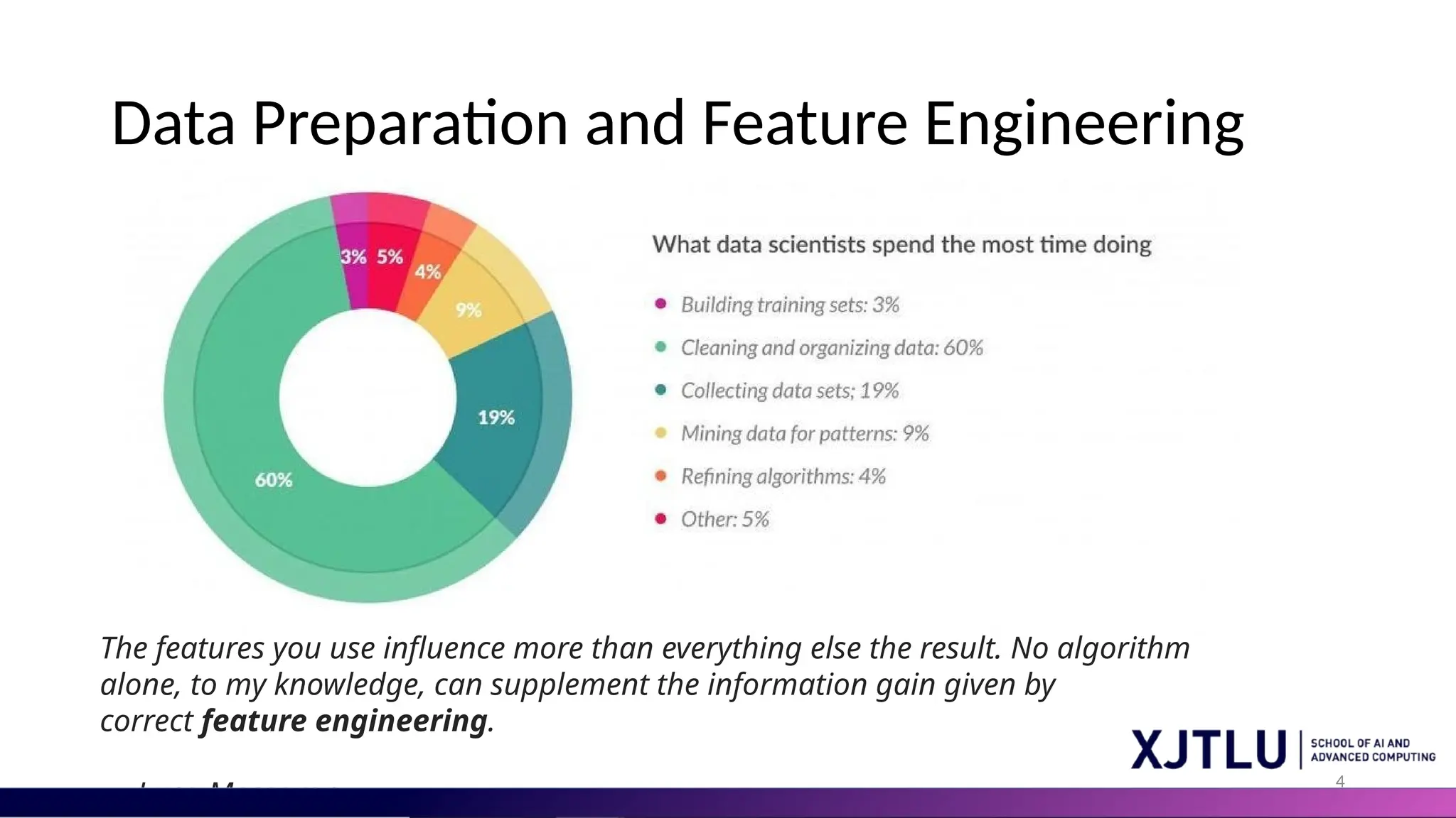
4 Data Preparation andFeature Engineering The features you use influence more than everything else the result. No algorithm alone, to my knowledge, can supplement the information gain given by correct feature engineering. — Luca Massaron
5.
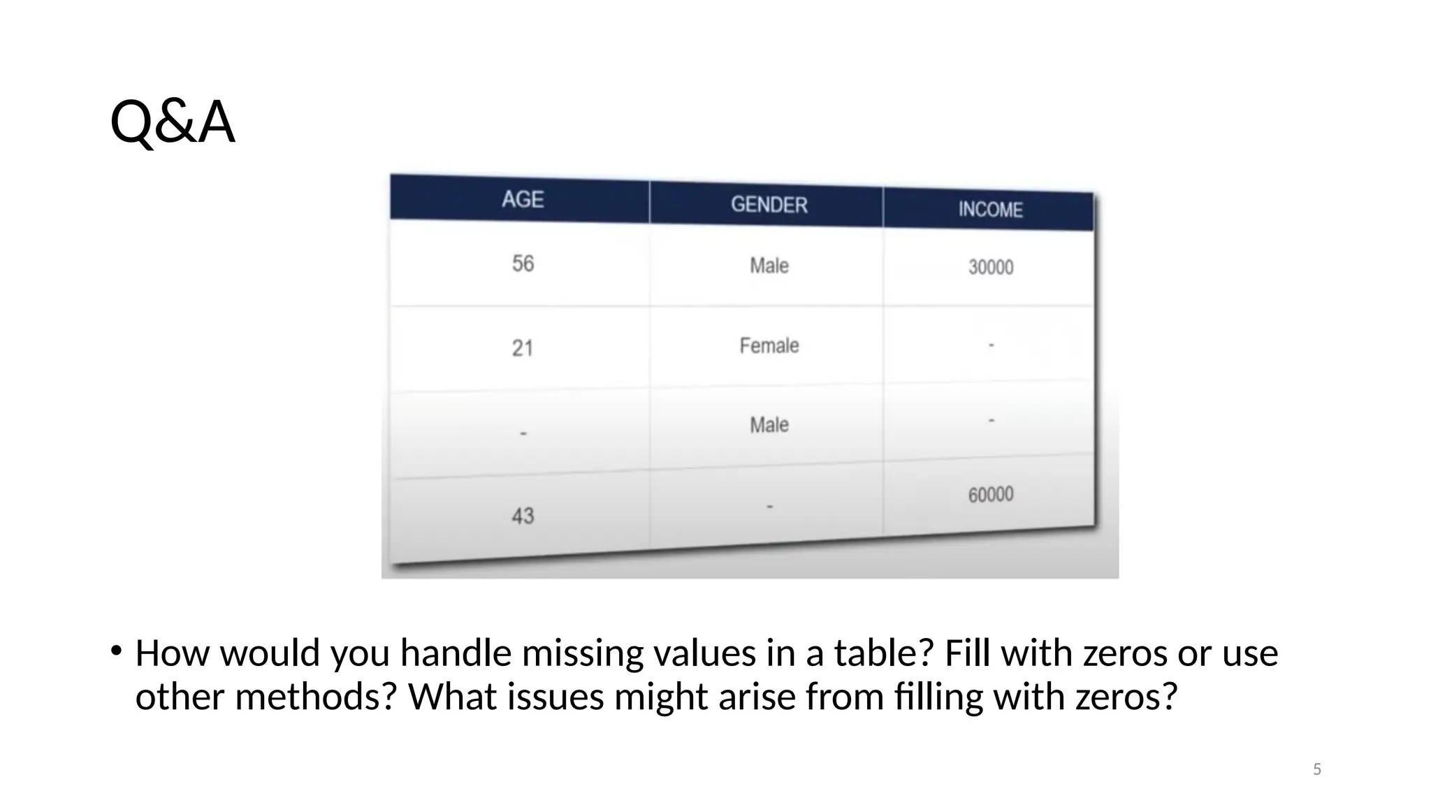
5 Q&A • How wouldyou handle missing values in a table? Fill with zeros or use other methods? What issues might arise from filling with zeros?
6.
6 Different types ofmissing values • 3 Main Types of Missing Data | Do THIS Before Handling Missing Valu es! – YouTube
7.
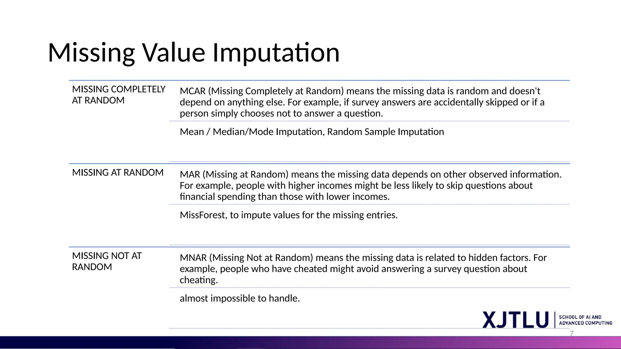
7 Missing Value Imputation MISSINGCOMPLETELY AT RANDOM MCAR (Missing Completely at Random) means the missing data is random and doesn't depend on anything else. For example, if survey answers are accidentally skipped or if a person simply chooses not to answer a question. Mean / Median/Mode Imputation, Random Sample Imputation MISSING AT RANDOM MAR (Missing at Random) means the missing data depends on other observed information. For example, people with higher incomes might be less likely to skip questions about financial spending than those with lower incomes. MissForest, to impute values for the missing entries. MISSING NOT AT RANDOM MNAR (Missing Not at Random) means the missing data is related to hidden factors. For example, people who have cheated might avoid answering a survey question about cheating. almost impossible to handle.
8.
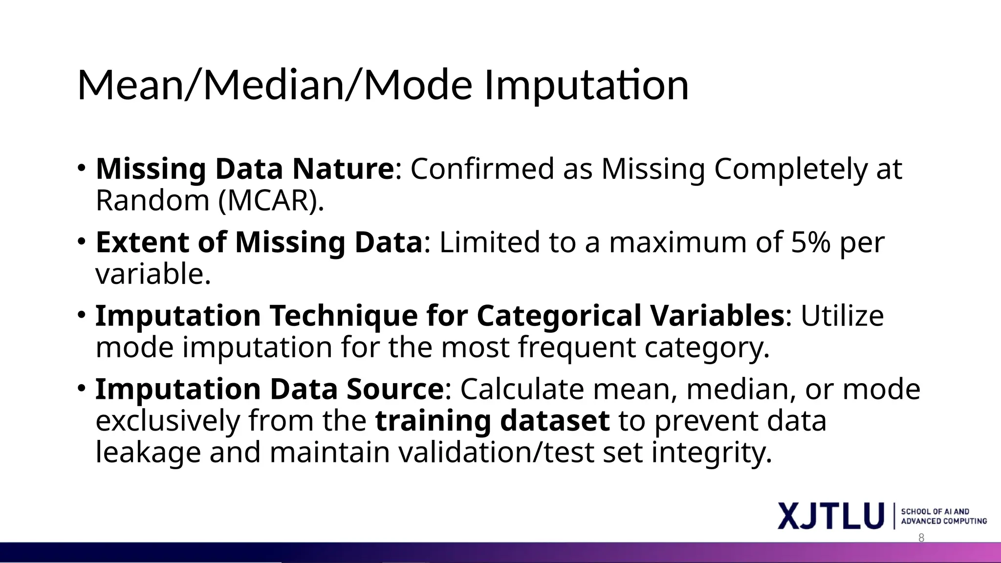
8 Mean/Median/Mode Imputation • MissingData Nature: Confirmed as Missing Completely at Random (MCAR). • Extent of Missing Data: Limited to a maximum of 5% per variable. • Imputation Technique for Categorical Variables: Utilize mode imputation for the most frequent category. • Imputation Data Source: Calculate mean, median, or mode exclusively from the training dataset to prevent data leakage and maintain validation/test set integrity.
9.
9 Regression Imputation –Miss Forest • Another great application of Random Forest! • Assume Data Missing At Random. • Utilizes entire dataset's information for imputation, enhancing the predictive accuracy of imputed values over simple mean/median/mode imputation
10.
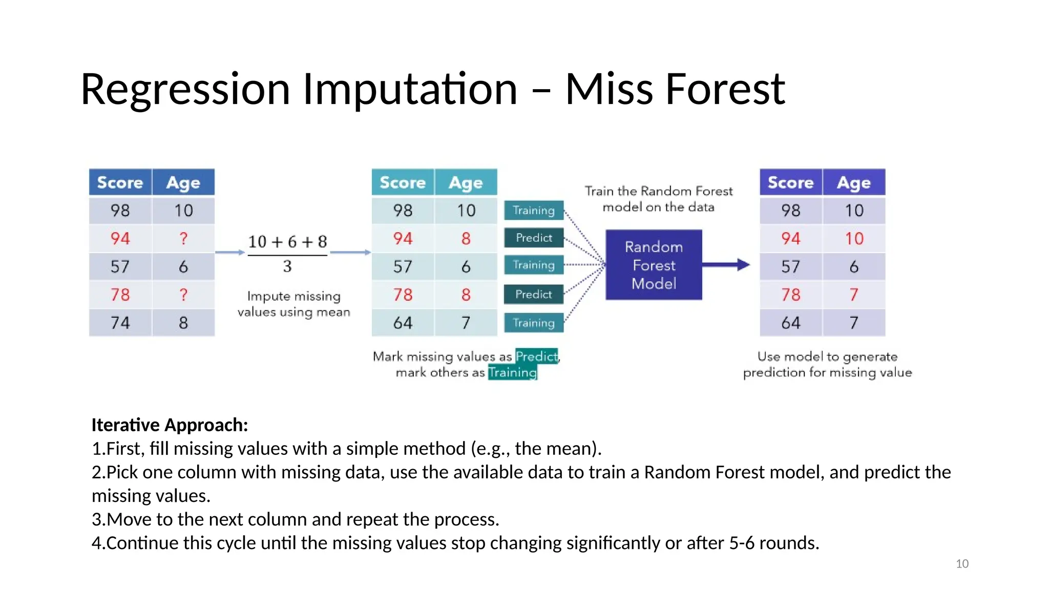
10 Regression Imputation –Miss Forest Iterative Approach: 1.First, fill missing values with a simple method (e.g., the mean). 2.Pick one column with missing data, use the available data to train a Random Forest model, and predict the missing values. 3.Move to the next column and repeat the process. 4.Continue this cycle until the missing values stop changing significantly or after 5-6 rounds.
11.
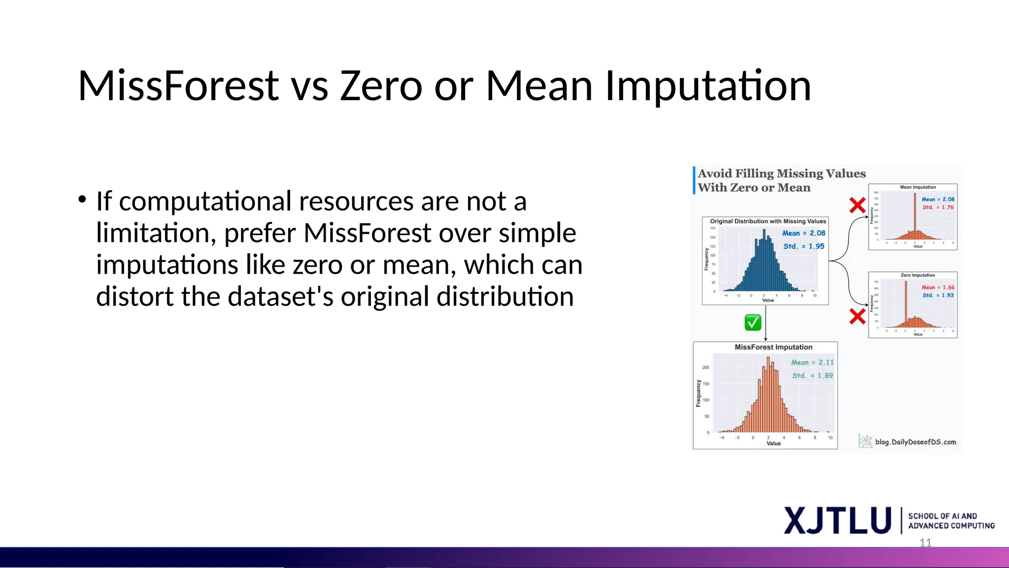
11 MissForest vs Zeroor Mean Imputation • If computational resources are not a limitation, prefer MissForest over simple imputations like zero or mean, which can distort the dataset's original distribution
12.
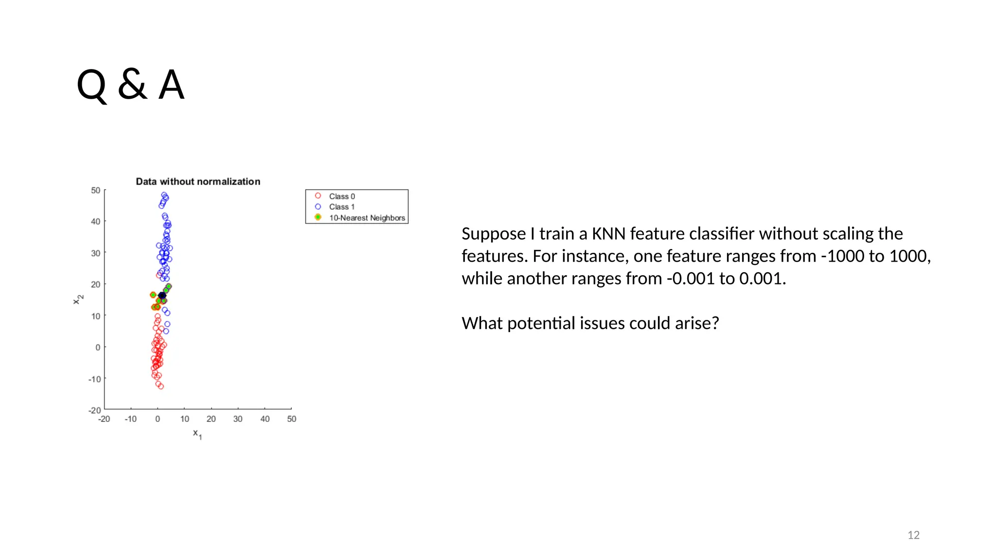
12 Q & A SupposeI train a KNN feature classifier without scaling the features. For instance, one feature ranges from -1000 to 1000, while another ranges from -0.001 to 0.001. What potential issues could arise?
13.
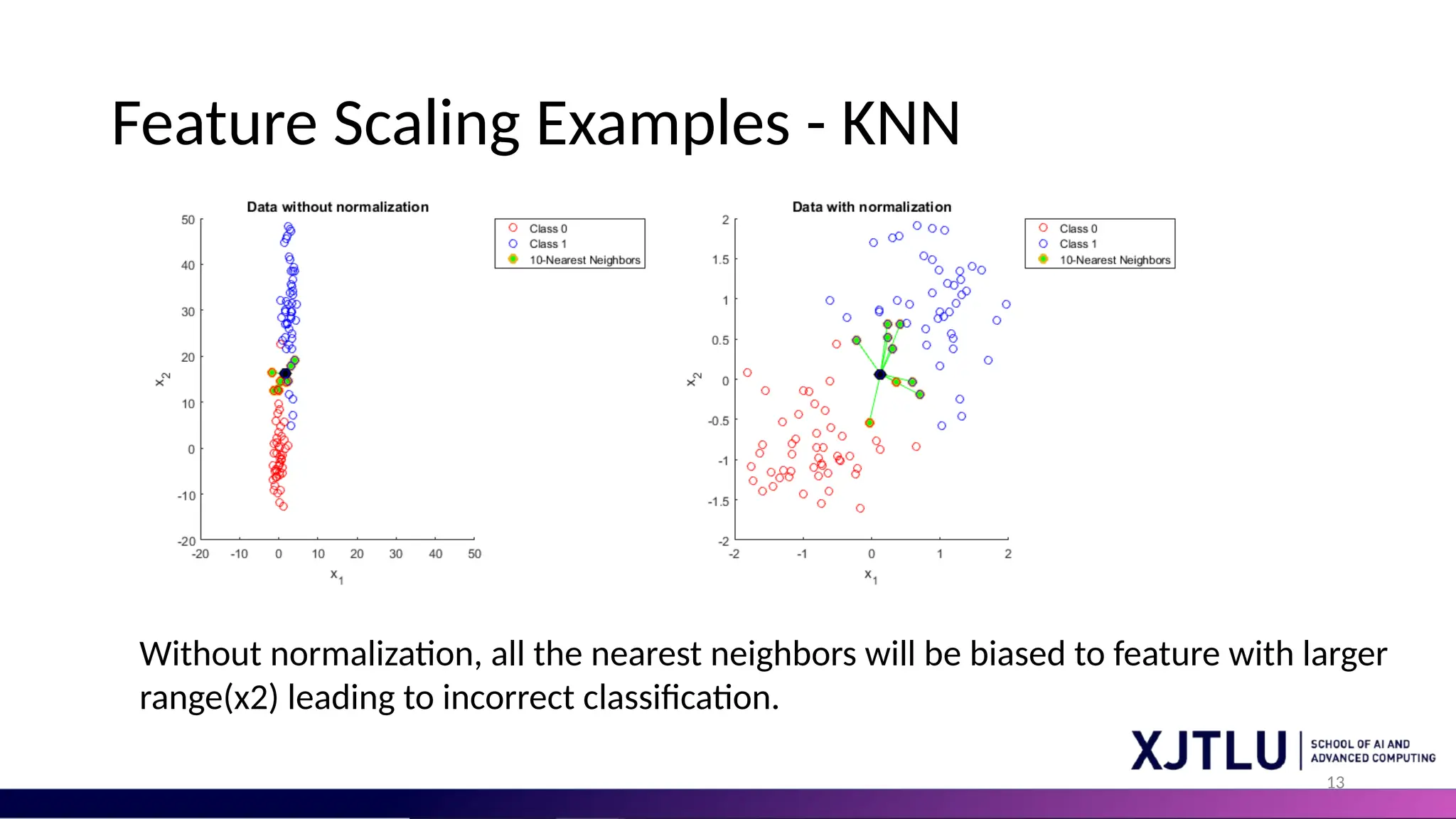
13 Feature Scaling Examples- KNN Without normalization, all the nearest neighbors will be biased to feature with larger range(x2) leading to incorrect classification.
14.
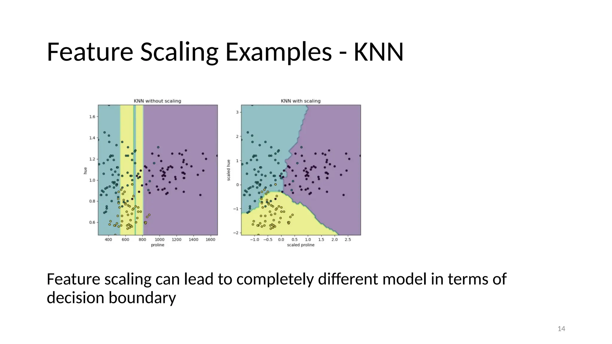
14 Feature Scaling Examples- KNN Feature scaling can lead to completely different model in terms of decision boundary
15.
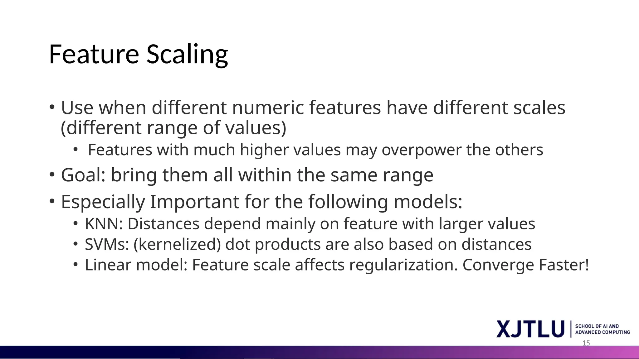
15 Feature Scaling • Usewhen different numeric features have different scales (different range of values) • Features with much higher values may overpower the others • Goal: bring them all within the same range • Especially Important for the following models: • KNN: Distances depend mainly on feature with larger values • SVMs: (kernelized) dot products are also based on distances • Linear model: Feature scale affects regularization. Converge Faster!
16.
16 Feature Scaling Standard Scalar Normalizes featuresto a standard Gaussian distribution. Centers the mean at 0 with a standard deviation of 1. Formula: x_scaled = (x – mean) / std_dev Use when data distribution is assumed to be normal. Min-Max Scaler: Scales features to a given range, often [0, 1]. Scales features to a given range, often [0, 1]. 、 Transforms all data points proportionally within the range x_scaled = (x – x_min) / (x_max – x_min) Use for scaling within a bounded range.
17.
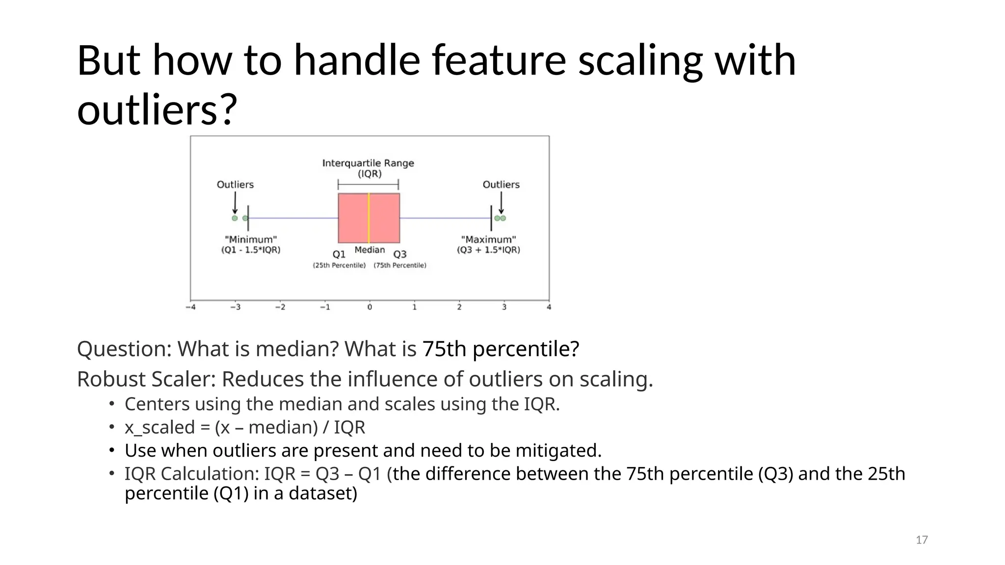
17 But how tohandle feature scaling with outliers? Question: What is median? What is 75th percentile? Robust Scaler: Reduces the influence of outliers on scaling. • Centers using the median and scales using the IQR. • x_scaled = (x – median) / IQR • Use when outliers are present and need to be mitigated. • IQR Calculation: IQR = Q3 – Q1 (the difference between the 75th percentile (Q3) and the 25th percentile (Q1) in a dataset)
18.
18 Q & A •Suppose you have a dataset with categorical features, such as 'dog' and 'cat'. Logistic regression, however, cannot directly handle categorical features. • To make these features compatible with the model, we might encode 'dog' as '0' and 'cat' as '1'. Is this a good approach? Why or why not?
19.
19 Categorical Feature Encoding •Ordinal encoding • For example, “Jan, Feb, Mar, Apr” • Simply assigns an integer value to each category in the order they are encountered • Only really useful if there exist a natural order in categories • Model will consider one category to be ‘higher’ or ‘closer’ to another
20.
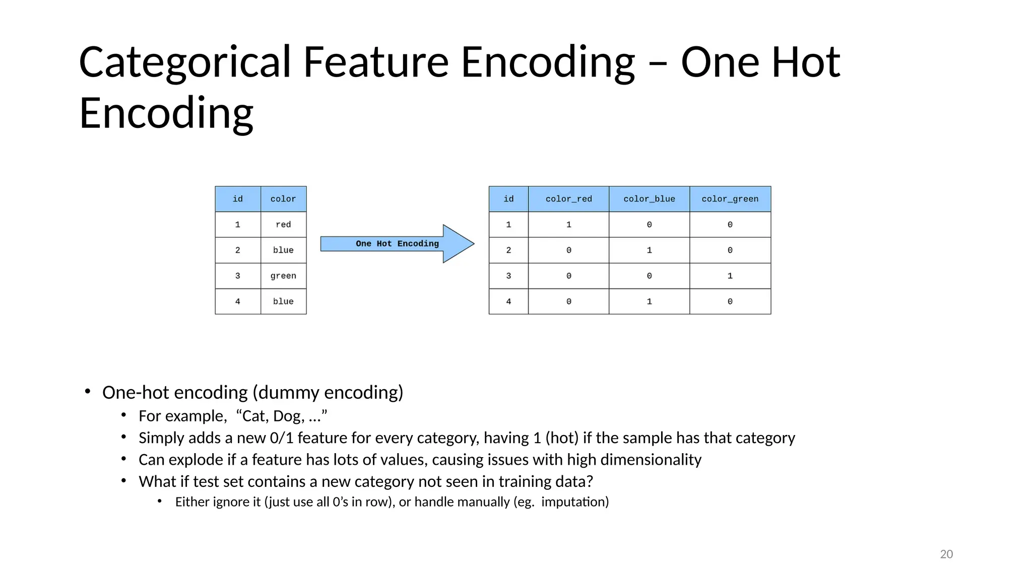
20 Categorical Feature Encoding– One Hot Encoding • One-hot encoding (dummy encoding) • For example, “Cat, Dog, …” • Simply adds a new 0/1 feature for every category, having 1 (hot) if the sample has that category • Can explode if a feature has lots of values, causing issues with high dimensionality • What if test set contains a new category not seen in training data? • Either ignore it (just use all 0’s in row), or handle manually (eg. imputation)
21.
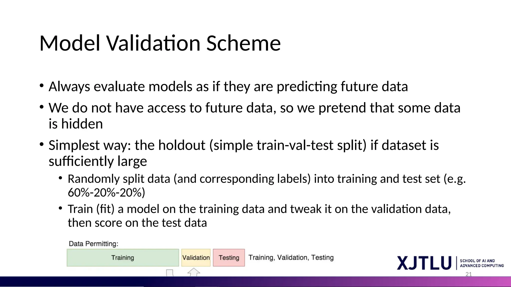
21 Model Validation Scheme •Always evaluate models as if they are predicting future data • We do not have access to future data, so we pretend that some data is hidden • Simplest way: the holdout (simple train-val-test split) if dataset is sufficiently large • Randomly split data (and corresponding labels) into training and test set (e.g. 60%-20%-20%) • Train (fit) a model on the training data and tweak it on the validation data, then score on the test data
22.
22 Q & A •What are issues with simple train-val-test split, when dataset is really small?
23.
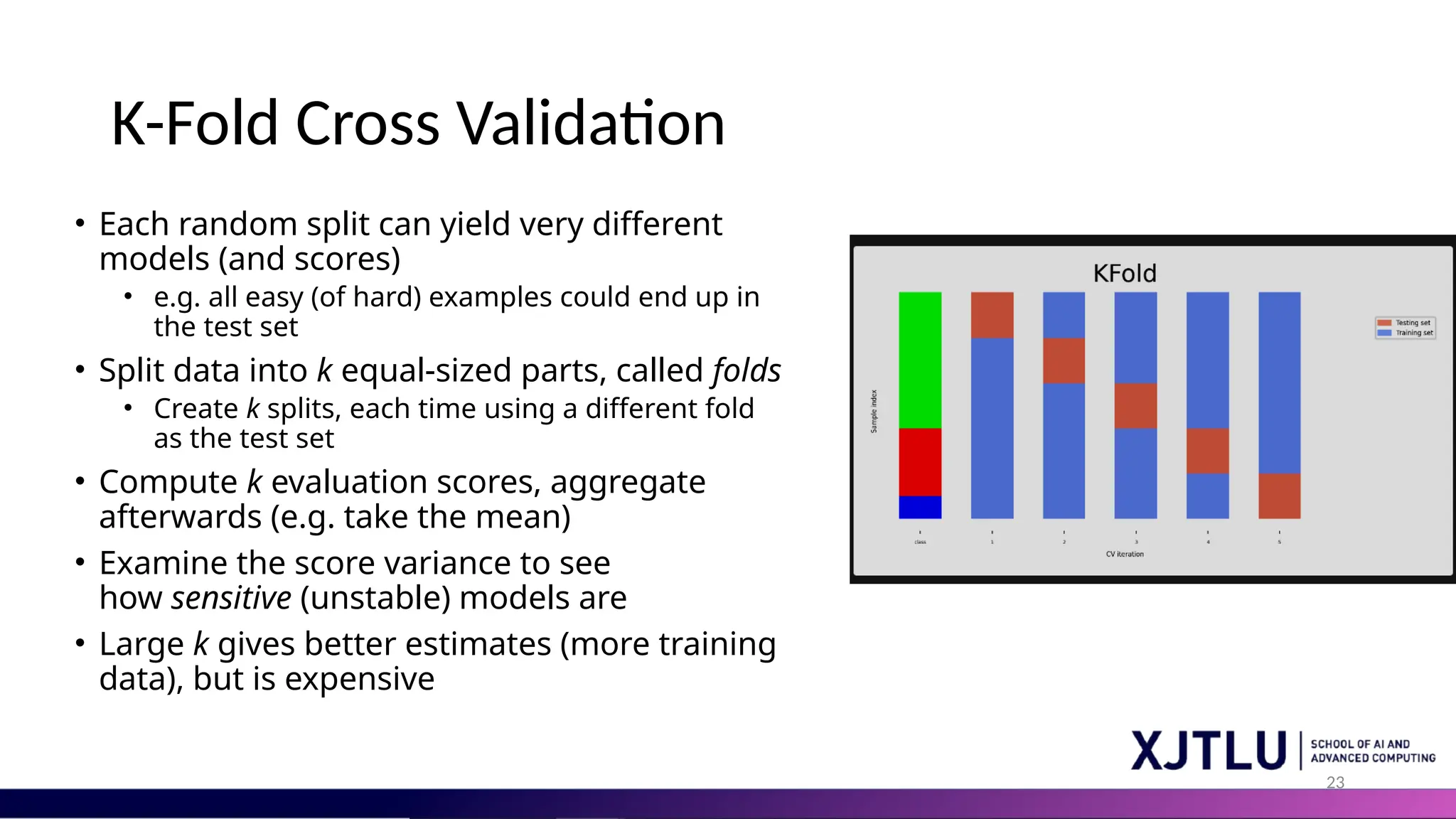
23 K-Fold Cross Validation •Each random split can yield very different models (and scores) • e.g. all easy (of hard) examples could end up in the test set • Split data into k equal-sized parts, called folds • Create k splits, each time using a different fold as the test set • Compute k evaluation scores, aggregate afterwards (e.g. take the mean) • Examine the score variance to see how sensitive (unstable) models are • Large k gives better estimates (more training data), but is expensive
24.
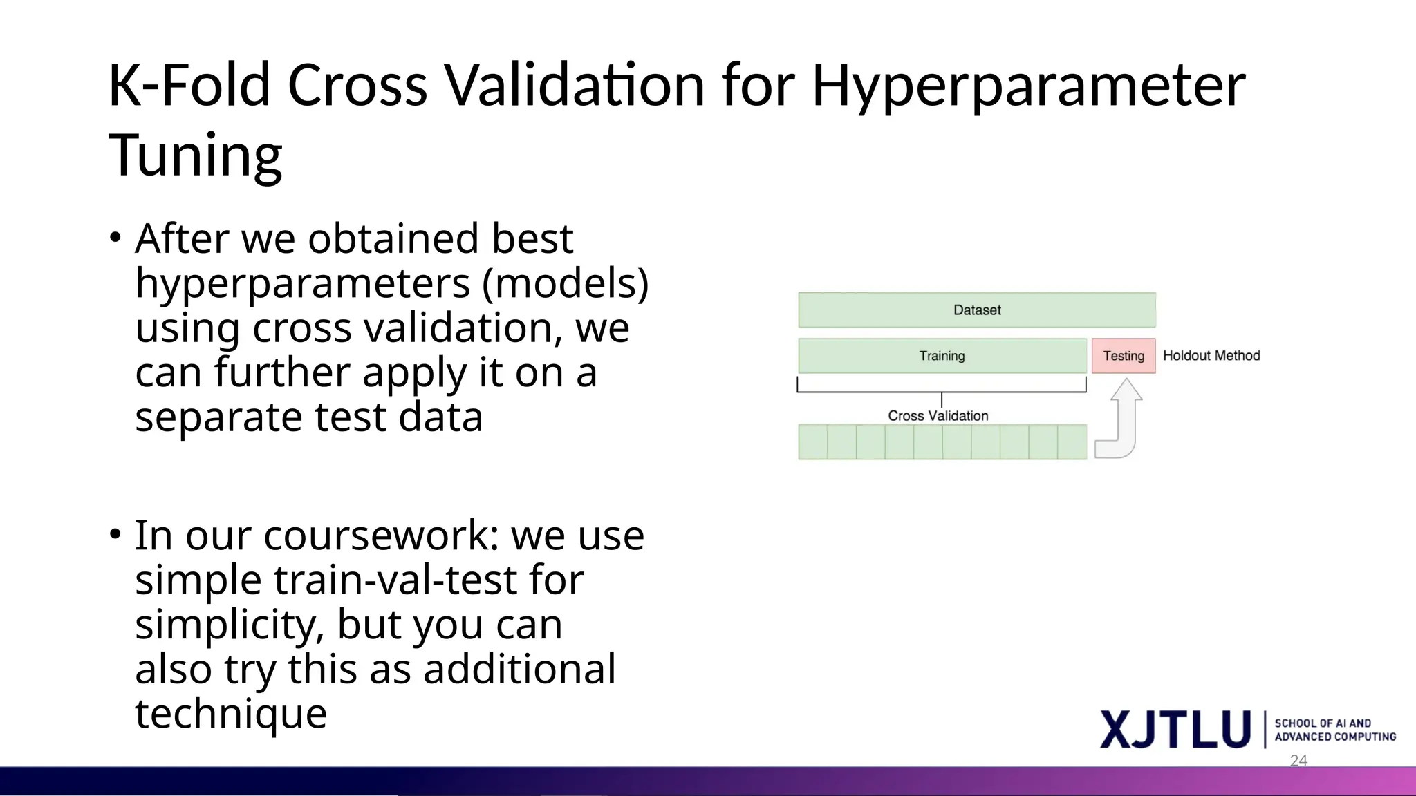
24 K-Fold Cross Validationfor Hyperparameter Tuning • After we obtained best hyperparameters (models) using cross validation, we can further apply it on a separate test data • In our coursework: we use simple train-val-test for simplicity, but you can also try this as additional technique
25.
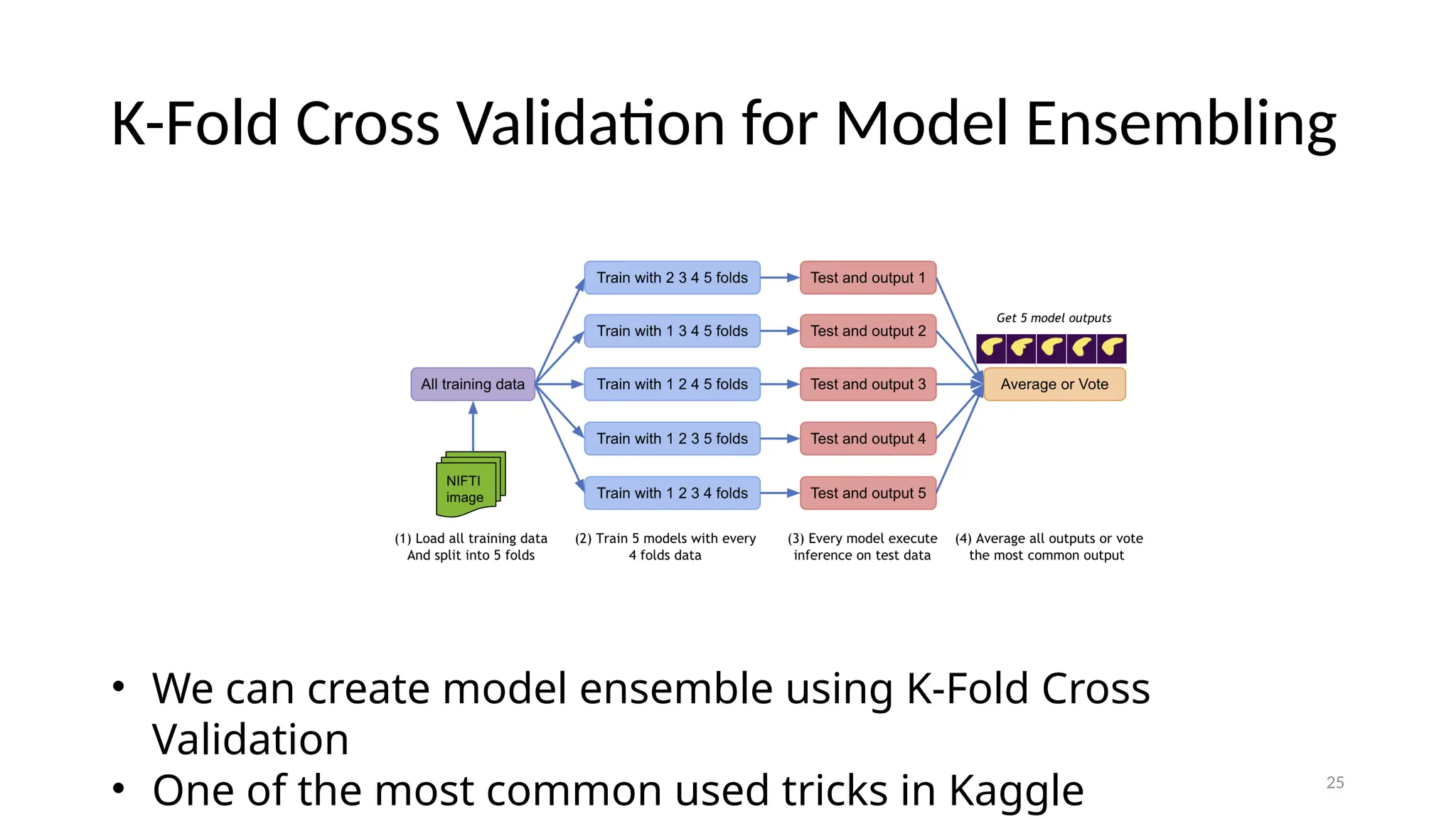
25 K-Fold Cross Validationfor Model Ensembling • We can create model ensemble using K-Fold Cross Validation • One of the most common used tricks in Kaggle
26.
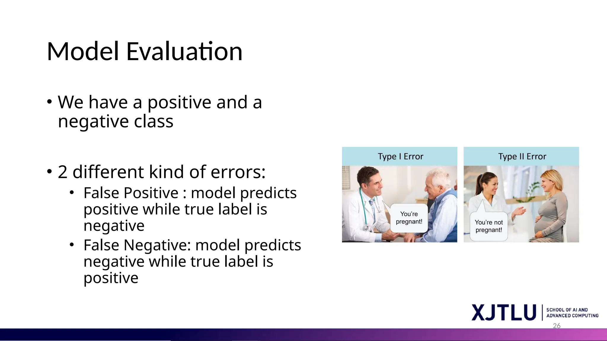
26 Model Evaluation • Wehave a positive and a negative class • 2 different kind of errors: • False Positive : model predicts positive while true label is negative • False Negative: model predicts negative while true label is positive
27.
27 Q&A • Suppose someonehas cancer but was not diagnosed (missed detection). • Suppose someone was healthy but was diagnosed with cancer (false detection). • What are the consequences? Which situation is more serious?
28.
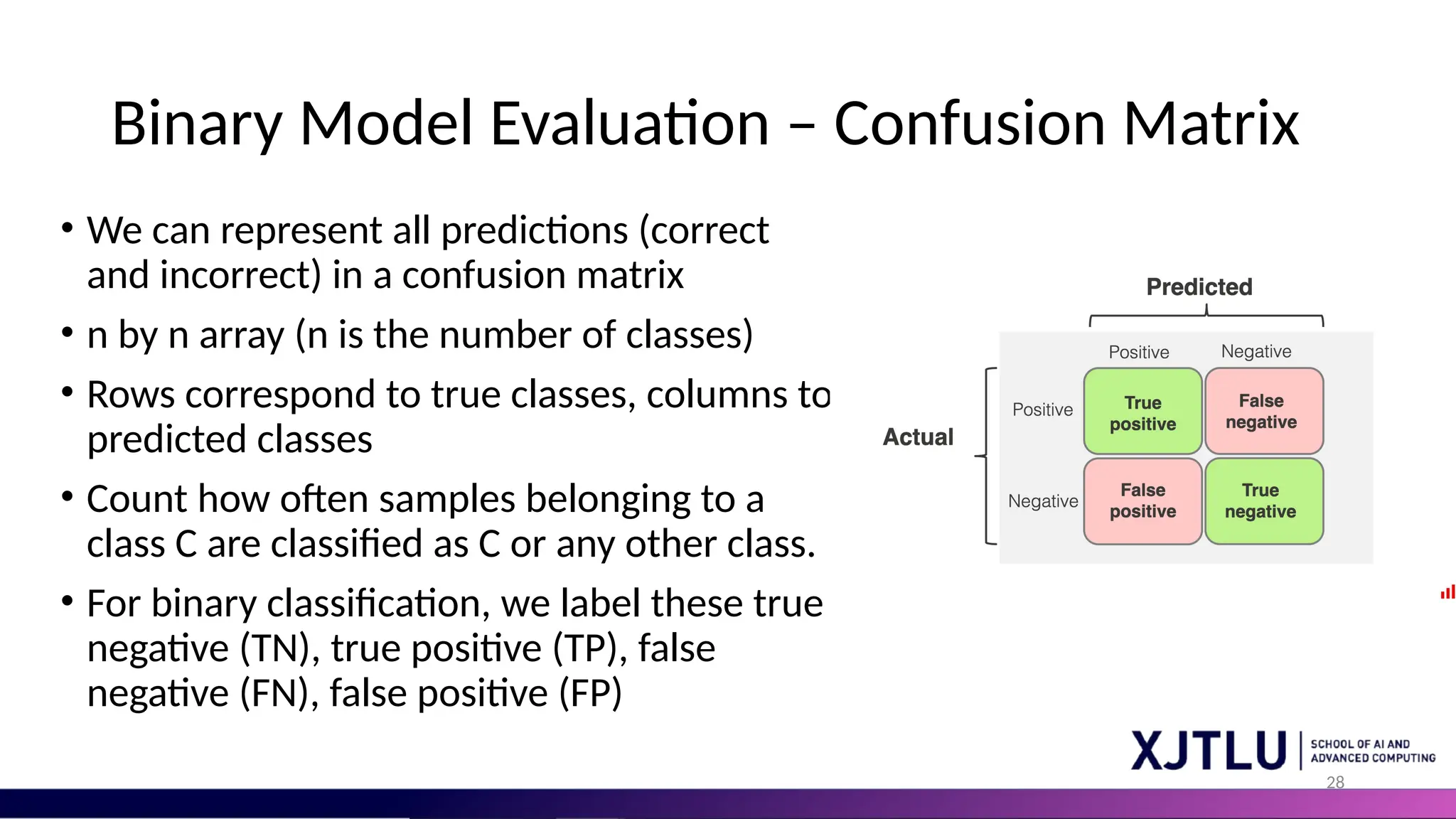
28 Binary Model Evaluation– Confusion Matrix • We can represent all predictions (correct and incorrect) in a confusion matrix • n by n array (n is the number of classes) • Rows correspond to true classes, columns to predicted classes • Count how often samples belonging to a class C are classified as C or any other class. • For binary classification, we label these true negative (TN), true positive (TP), false negative (FN), false positive (FP)
29.
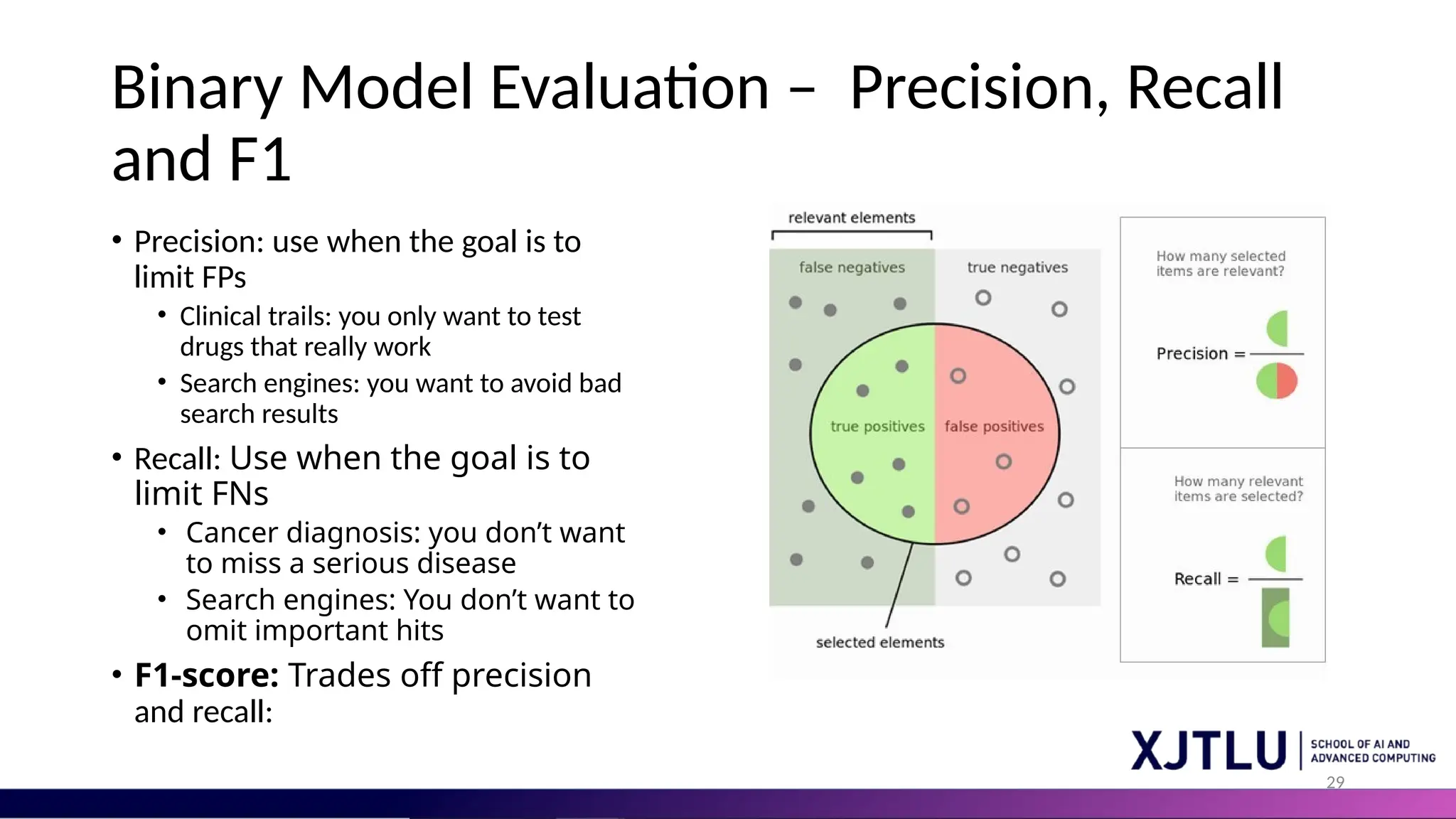
29 Binary Model Evaluation– Precision, Recall and F1 • Precision: use when the goal is to limit FPs • Clinical trails: you only want to test drugs that really work • Search engines: you want to avoid bad search results • Recall: Use when the goal is to limit FNs • Cancer diagnosis: you don’t want to miss a serious disease • Search engines: You don’t want to omit important hits • F1-score: Trades off precision and recall:
30.
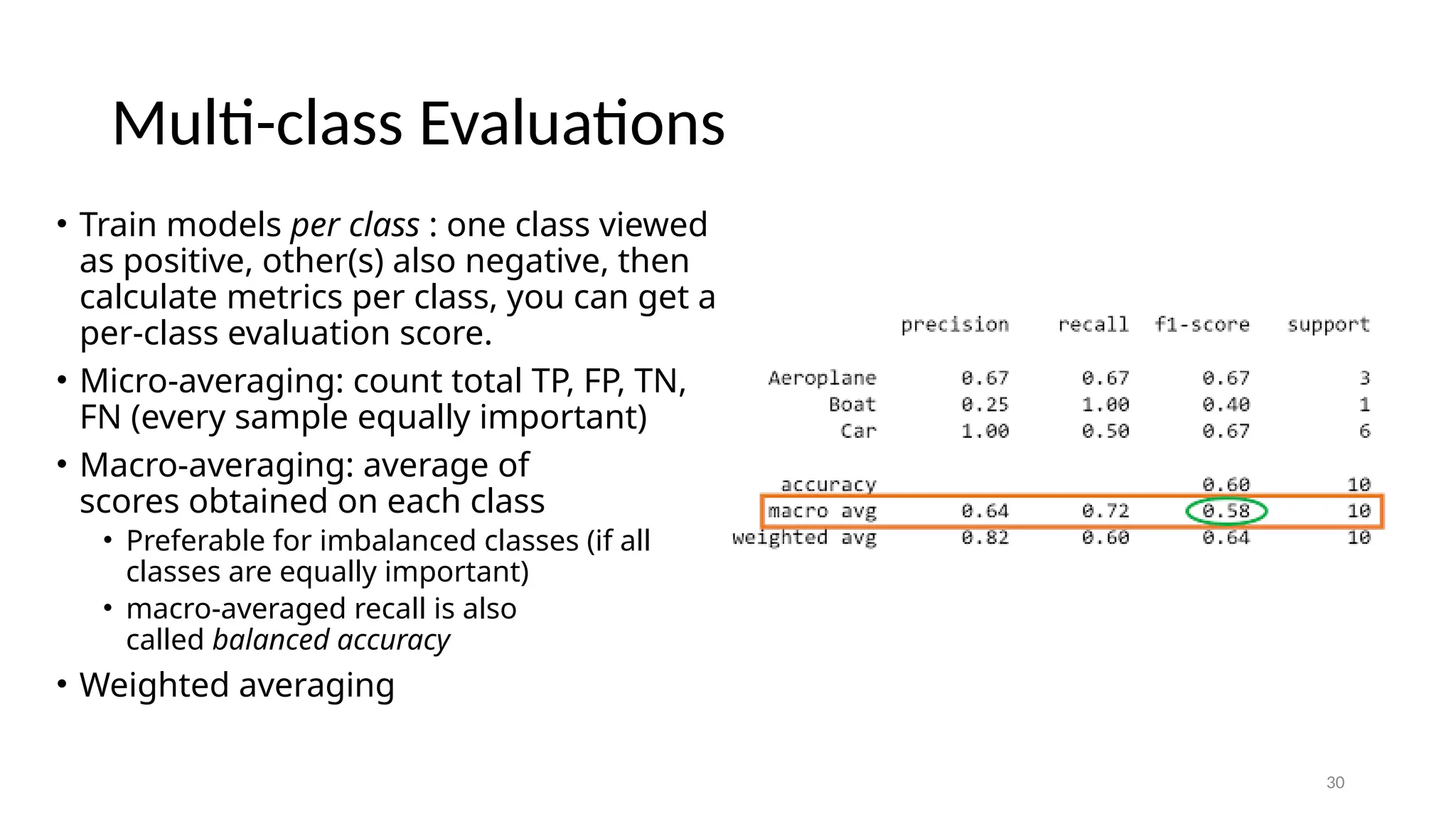
30 Multi-class Evaluations • Trainmodels per class : one class viewed as positive, other(s) also negative, then calculate metrics per class, you can get a per-class evaluation score. • Micro-averaging: count total TP, FP, TN, FN (every sample equally important) • Macro-averaging: average of scores obtained on each class • Preferable for imbalanced classes (if all classes are equally important) • macro-averaged recall is also called balanced accuracy • Weighted averaging
31.
31 Summary • We discussvarious feature engineering techniques, including feature scaling, missing value imputation, outlier handling and categorial feature encoding • We discuss the model selection and evaluation procedure, specifically cross-validation and evaluation metrics.
Editor's Notes
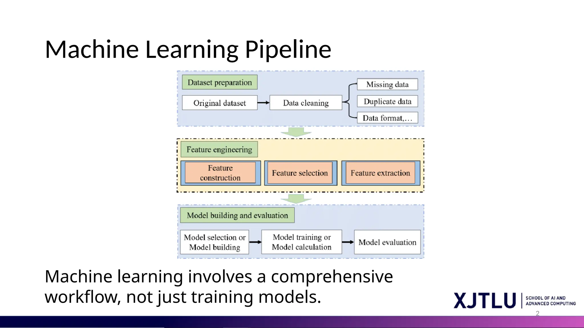
#2 In today’s lecture, we'll explore the workflow of a typical machine learning system, encompassing preprocessing of raw data, feature scaling, encoding, discretization, label imbalance correction, feature selection, dimensionality reduction, and learning and evaluation, which includes acknowledging algorithm biases, model selection, data splitting, and ultimately prediction, to form an integrated pipeline that prepares data for learning and optimizes model performance.
#4 What is a feature and why we need the engineering of it? Basically, all machine learning algorithms use some input data to create outputs. This input data comprise features, which are usually in the form of structured columns. Algorithms require features with some specific characteristic to work properly. Here, the need for feature engineering arises. I think feature engineering efforts mainly have two goals: Preparing the proper input dataset, compatible with the machine learning algorithm requirements. Improving the performance of machine learning models. According to a survey in Forbes, data scientists spend 80% of their time on data preparation.
#7 In data analysis, dealing with missing data is a common challenge, and the approach to imputation often depends on the nature of the missingness. With Missing Completely at Random (MCAR), the absence of data is independent of both observed and unobserved data, akin to survey responses being accidentally skipped during data entry or respondents choosing to leave a question blank without any systematic bias. Simple methods like imputing the mean, median, or mode, or using a random sample, can be effective for MCAR since the missingness does not introduce a systemic distortion. In contrast, Missing at Random (MAR) occurs when the propensity for missing data is related to other, observed data. For instance, a pattern where one gender omits answers to questions about parental leave more frequently than the other. In such cases, more sophisticated techniques like MissForest can be employed, which predict missing values using patterns found in other variables. However, when dealing with Missing Not at Random (MNAR), the problem becomes more complex, as the missing data is related to factors not captured in the dataset. For example, individuals who have been unfaithful may avoid questions about fidelity. Addressing MNAR effectively is particularly challenging because the very nature of the missing data is obscured by unobserved influences, resisting standard imputation methods.
#9 Assuming data is Missing at Random (MAR), one can utilize more sophisticated imputation methods that leverage the entire dataset, potentially resulting in greater predictive accuracy than would be achieved with simple mean, median, or mode imputation.
#10 An iterative approach begins by filling in missing values with a basic imputation, such as the mean of the observed values. The dataset is then split: a portion with complete data is used for training, while the subset with previously imputed values is treated as the target for prediction. A Random Forest algorithm, known for its robustness, is applied to predict the missing values, which are then updated with these predictions. This cycle is repeated, progressively refining the quality of the data with each iteration, until the imputations stabilize and no significant changes occur, or until a predetermined number of iterations is reached. This iterative process ensures that each round of imputation benefits from the enhanced patterns and relationships uncovered in the data from the previous round.
#13 Without normalization of feature scales, machine learning algorithms that rely on distance calculations, such as K-Nearest Neighbors (KNN), can be significantly biased. In cases where one feature has a much smaller range than others, the nearest neighbors tend to be affected stronger by x2. This misalignment occurs because the larger-scaled features overpower the smaller ones, causing the distance metric to be skewed in favor of the larger ranges. Consequently, this leads to incorrect classification or prediction results, as the model essentially overlooks the contributions of features with smaller ranges. Normalization ensures that each feature contributes equally to the distance computations, thereby preventing the axis with the smaller range from disproportionately determining the nearest neighbors.
#15 When your data has numeric features that vary widely in scale, some features with higher numerical values might dominate over others during the modeling process, skewing the results. The aim is to level the playing field by bringing every feature into the same range of values. This step is particularly crucial for models like K-Nearest Neighbors (KNN), where the calculation of distances can be heavily biased towards the feature with the larger scale. Similarly, Support Vector Machines (SVMs) rely on dot products when kernelized, which again depend on the distances between data points. Even in linear models, the scale of features can influence how regularization is applied. Normalizing or standardizing these features ensures that each one contributes equally to the model's performance, allowing for a more accurate and fair analysis.
#16 In data preprocessing, the Standard Scaler is a tool that normalizes features to fit a standard Gaussian distribution, aligning the mean at 0 and standard deviation at 1, using the transformation �scaled=(�−mean)std_devxscaled=std_dev(x−mean). This is particularly effective when the data is assumed to follow a normal distribution. On the other hand, the Min-Max Scaler adjusts features to fall within a specific range, typically between 0 and 1, according to the formula �scaled=(�−�min)(�max−�min)xscaled=(xmax−xmin)(x−xmin), ensuring all values are proportionately adjusted within this bounded interval, which is ideal for when scaling needs to adhere to a predefined range.
#17 . The Robust Scaler, however, is designed to be insensitive to outliers by using the median and the interquartile range (IQR) for centering and scaling, respectively, as expressed by �scaled=(�−median)IQRxscaled=IQR(x−median), where IQR is the range between the 75th and 25th percentiles. This scaler is useful in datasets where outliers could skew the scaling process. The median is the middle number when you put all your numbers in order. The 25% percentile is the value where one-quarter of the numbers are below it.
#19 Ordinal encoding and one-hot encoding are two methods for converting categorical data into numerical form for machine learning models. Ordinal encoding assigns an integer to each category based on the order they are encountered, which is beneficial if the categories have a natural ranking—for instance, the months "Jan, Feb, Mar, Apr" could be encoded as 1, 2, 3, 4, respectively. However, this technique implies a hierarchy where some categories are considered 'higher' or 'closer' to others, which may not always be appropriate. On the other hand, one-hot encoding creates a new binary feature for each category, which is set to 1 (hot) if the sample belongs to that category, and 0 otherwise, as seen with categories like "Cat, Dog." While this method avoids implying any order, it can result in a high number of features, especially if the categorical variable has many unique values, leading to high dimensionality problems. Additionally, if new categories appear in the test set that weren't present in the training data, they must be either ignored or handled manually, such as through imputation, to ensure the model can process them.

![16 Feature Scaling Standard Scalar Normalizes features to a standard Gaussian distribution. Centers the mean at 0 with a standard deviation of 1. Formula: x_scaled = (x – mean) / std_dev Use when data distribution is assumed to be normal. Min-Max Scaler: Scales features to a given range, often [0, 1]. Scales features to a given range, often [0, 1]. 、 Transforms all data points proportionally within the range x_scaled = (x – x_min) / (x_max – x_min) Use for scaling within a bounded range.](https://image.slidesharecdn.com/lecture5buildmachinelearningsystem-250303160525-689c1da3/75/Build_Machine_Learning_System-for-Machine-Learning-Course-16-2048.jpg)