Download to read offline


![RCE-NN Steps ▪ Step2: FlatBuffer to C-byte Array ✓ MCUs in edge devices lack native filesystem support. Hence, we cannot load and execute the regular format (“.h5”, “.pb”, “.tflite”, etc.) trained CNNs ✓ We convert the quantized version of the trained model into a C array and compile it along with the program for the IoT application which is to be executed on the edge device Translated C byte array: unsigned char converted_quantised_model [] = { 0x18, 0x00, 0x00, 0x00, 0x54, 0x46, 0x4c, 0x33, 0x00, 0x00, 0x0e, 0x00, ... ... … }; unsigned int converted_quantised model_len = 21200; Command: xxd -i converted_quantised_ model file > translated c byte array of model.cc Method to translate the trained model into a C byte array](https://image.slidesharecdn.com/deep-cnn-optimization-ecml-tutorial-211205125702/75/ECML-PKDD-2021-ML-meets-IoT-Tutorial-Part-III-Deep-Optimizations-of-CNNs-and-Efficient-Deployment-on-IoT-Devices-27-2048.jpg)


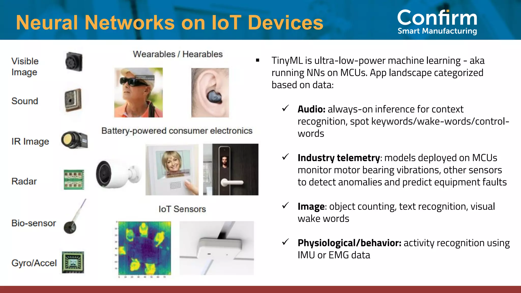
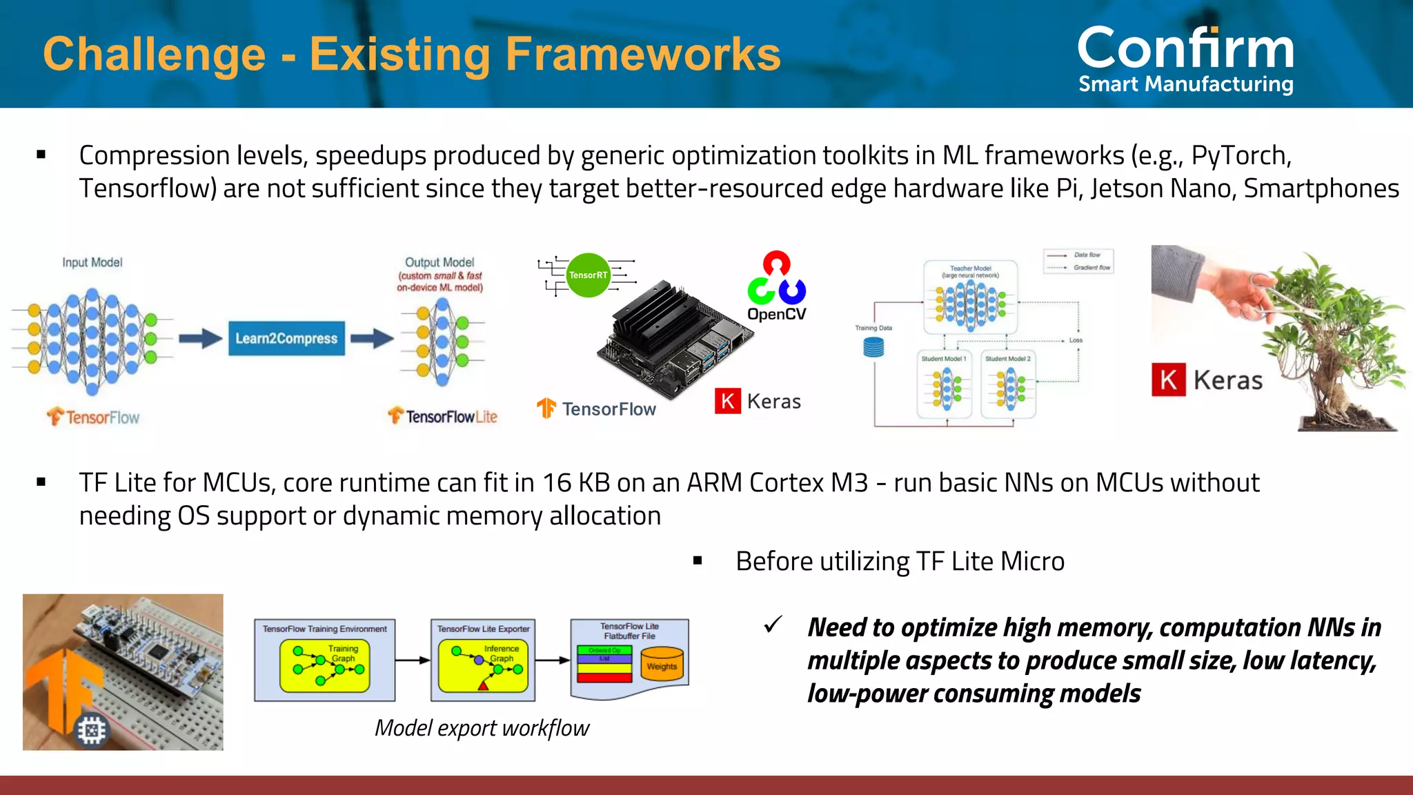
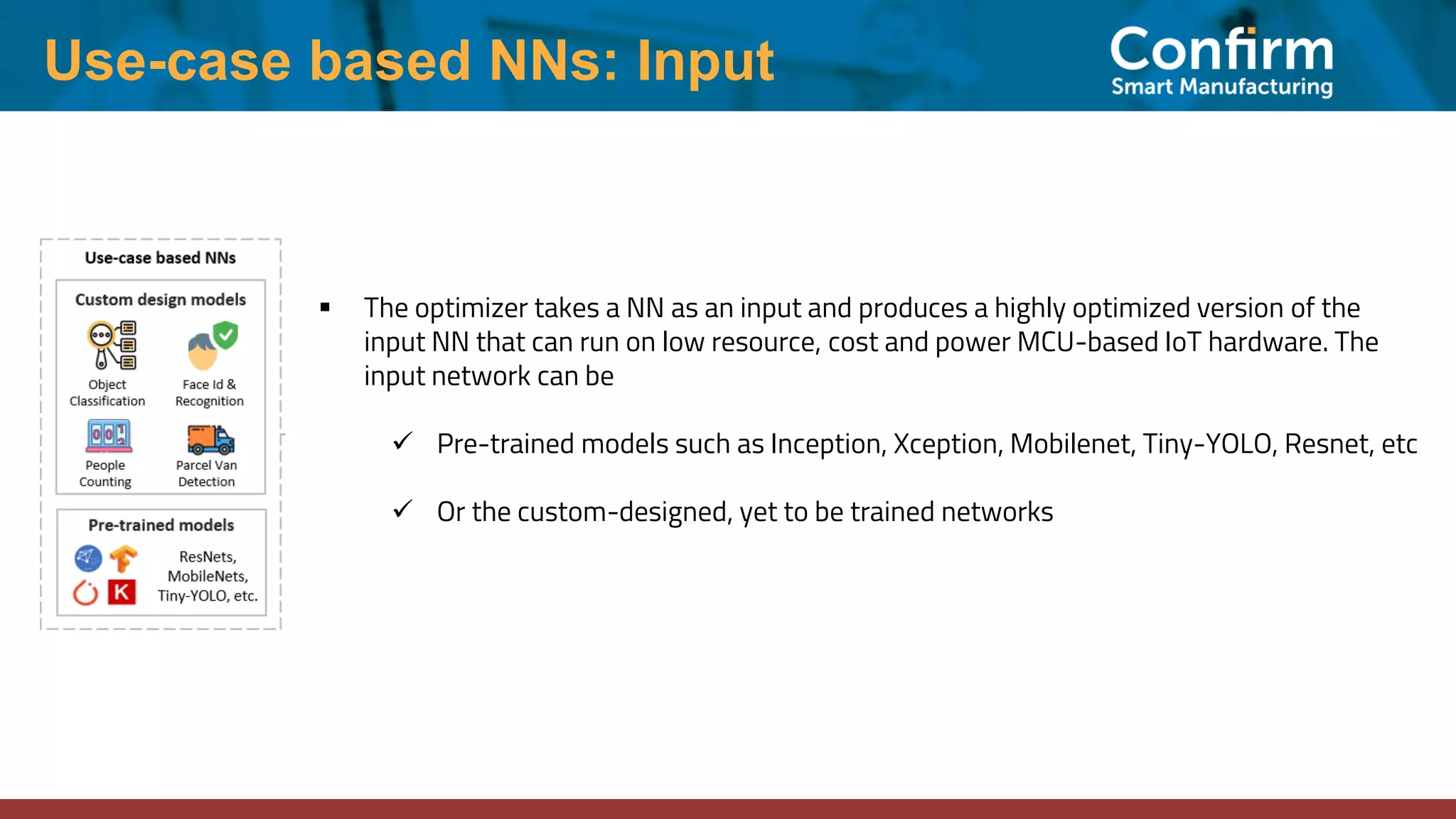
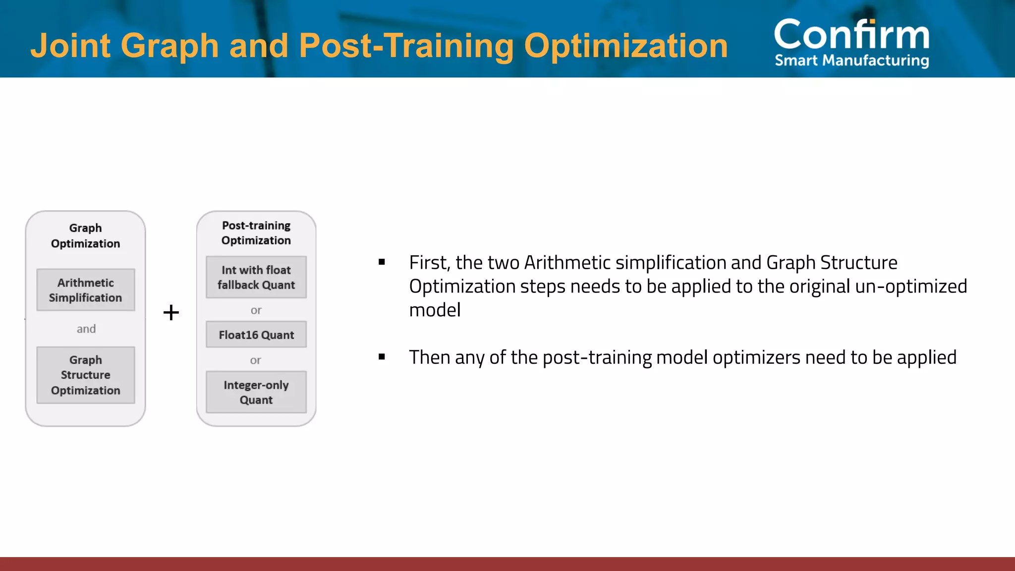
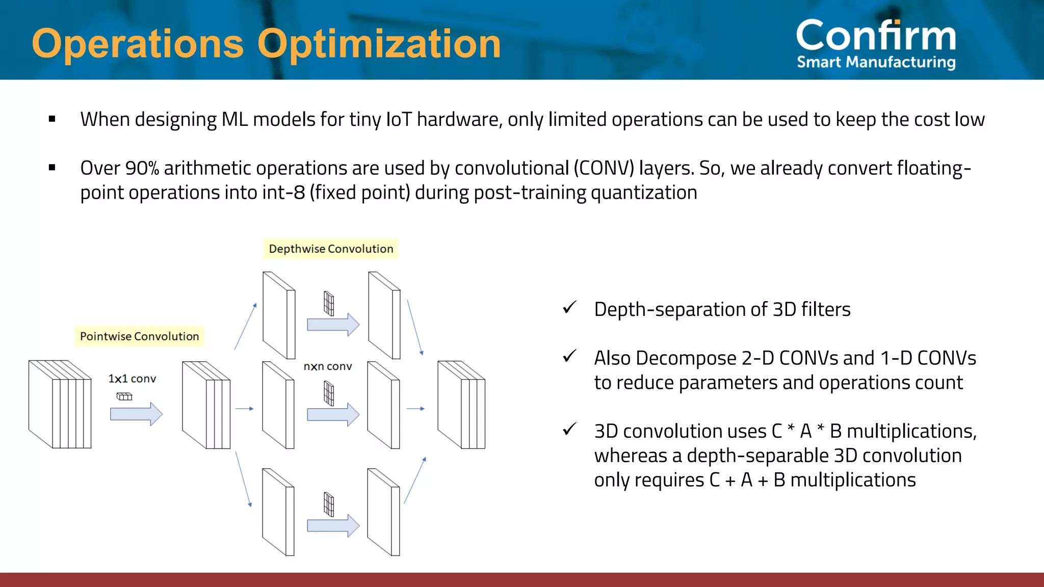
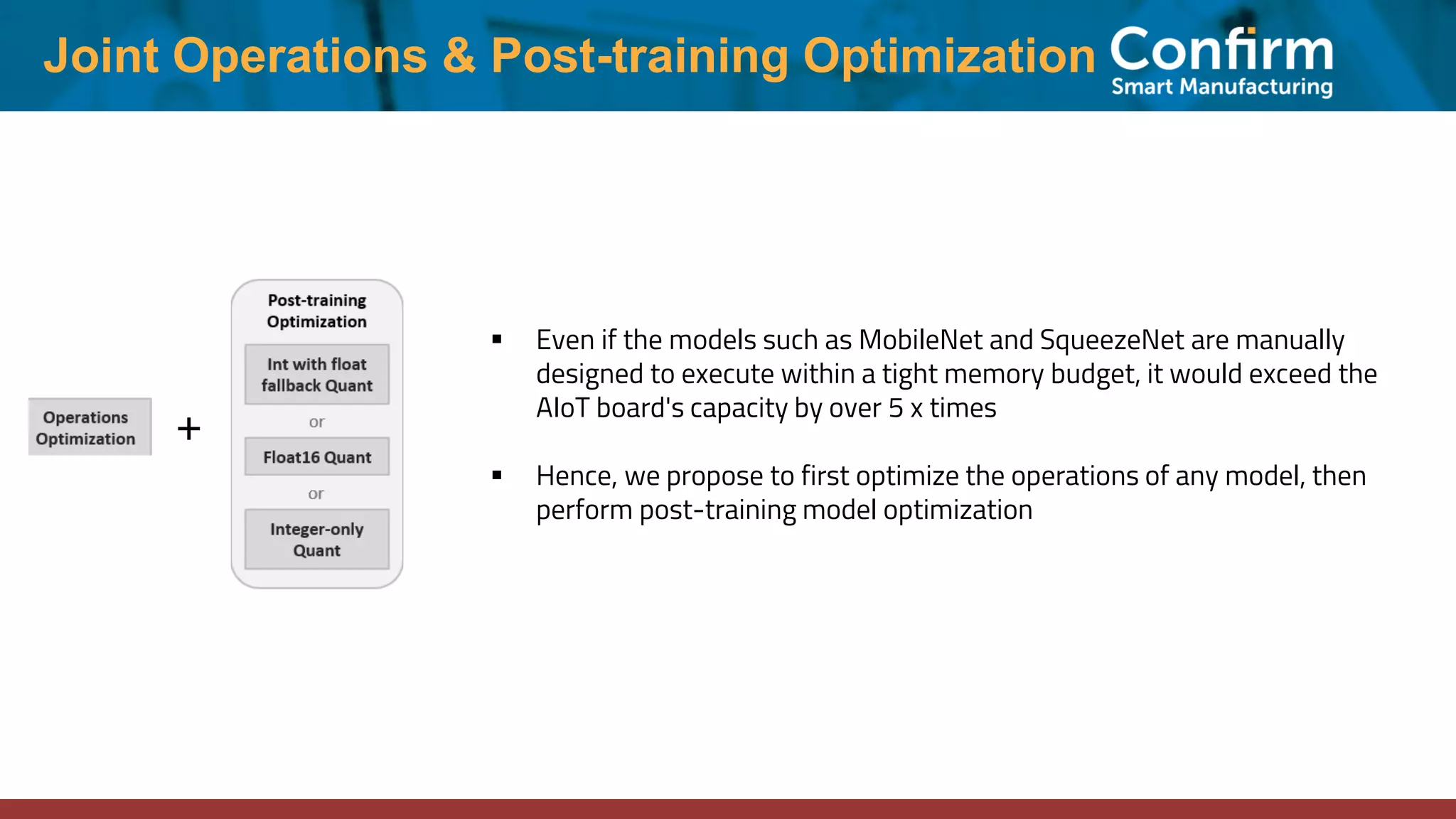
This document discusses optimizing neural networks for deployment on Internet of Things (IoT) devices. It describes several challenges, including existing frameworks not being optimized enough for low-powered IoT hardware. It then outlines various state-of-the-art optimization techniques, including pruning, quantization, graph optimizations, and replacing operations. Finally, it proposes a multi-stage optimization pipeline that first applies pre-training, post-training, graph, and operations optimizations, and then combines multiple techniques for deeper optimization levels to maximize size and speed improvements while preserving accuracy.