Download as PDF, PPTX


![Convolutional Encoder - Polynomial description • Similarly, encoder can also be expressed as polynomial of D. • Using previous problem, ko =1, no= 2, – first bit of code g11(D)= D2+D+1 – Second bit of code g12(D)= D2+1 – G(D) = [gij(D)]= [D2+D+1 D2+1] cj(D) = ∑i il(D)gl,j(D) C(D) = I(D)G(D)](https://image.slidesharecdn.com/convolutioncodes-160208053008/75/Convolution-codes-Coding-Decoding-Tree-codes-and-Trellis-codes-for-multiple-error-correction-15-2048.jpg)
![Convolutional encoder – Example k0 = 1, n0 = 2, rate = ½. G(D) = [1 D4+1] Called systematic convolution encoder as k0 bits of code are same as data.](https://image.slidesharecdn.com/convolutioncodes-160208053008/75/Convolution-codes-Coding-Decoding-Tree-codes-and-Trellis-codes-for-multiple-error-correction-17-2048.jpg)
![Convolutional encoder – Formal definitions Wordlength k = k0 maxi,j{deg gij (D) + 1]. Blocklength n = n0 maxi,j{deg gij (D) + 1]. Constraint length v = ∑ maxi,j{deg gij (D)]. Parity Check matrix H(D) is (n0-k0) by n0 matrix of polynomials which satisfies- G(D) H(D)- 1= 0 Syndrome polynomial s(D) is (n0-k0) component row vector s(D) = v(D) H(D)- 1](https://image.slidesharecdn.com/convolutioncodes-160208053008/75/Convolution-codes-Coding-Decoding-Tree-codes-and-Trellis-codes-for-multiple-error-correction-20-2048.jpg)
![Convolutional encoder – Formal definitions Systematic Encoder has G(D) = [I | P(D)] Where I is k0 by ko identity matrix and P(D) is ko by ( n0-k0) parity check polynomial given by H(D) = [-P(D)T |I] Where I is ( n0-k0) by( n0-k0) identity matrix. Also G(D) H(D)T = 0](https://image.slidesharecdn.com/convolutioncodes-160208053008/75/Convolution-codes-Coding-Decoding-Tree-codes-and-Trellis-codes-for-multiple-error-correction-21-2048.jpg)
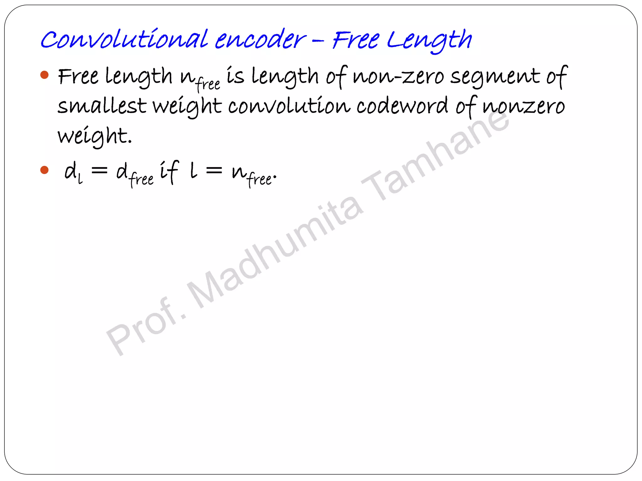
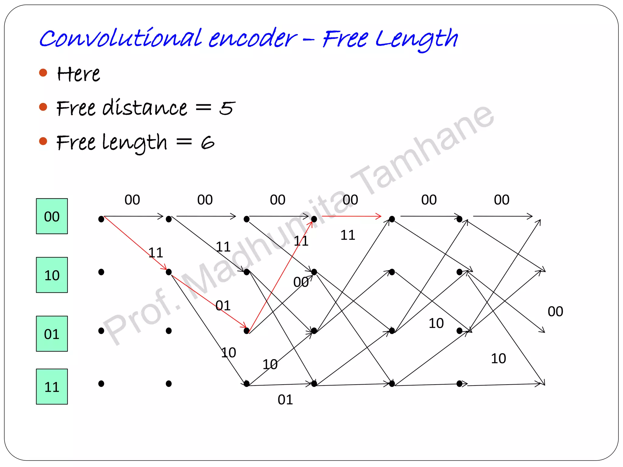
![Convolutional encoder – Free Distance Minimum distance between arbitrarily long encoded sequence. ( Possibly infinite) Free distance is dfree = maxl[dj] It can be minimum weight of a path that deviates from the all zero path and later merges back into the all zero path. Also dm+1 ≤ dm+2 ≤ …≤ dfree](https://image.slidesharecdn.com/convolutioncodes-160208053008/75/Convolution-codes-Coding-Decoding-Tree-codes-and-Trellis-codes-for-multiple-error-correction-24-2048.jpg)
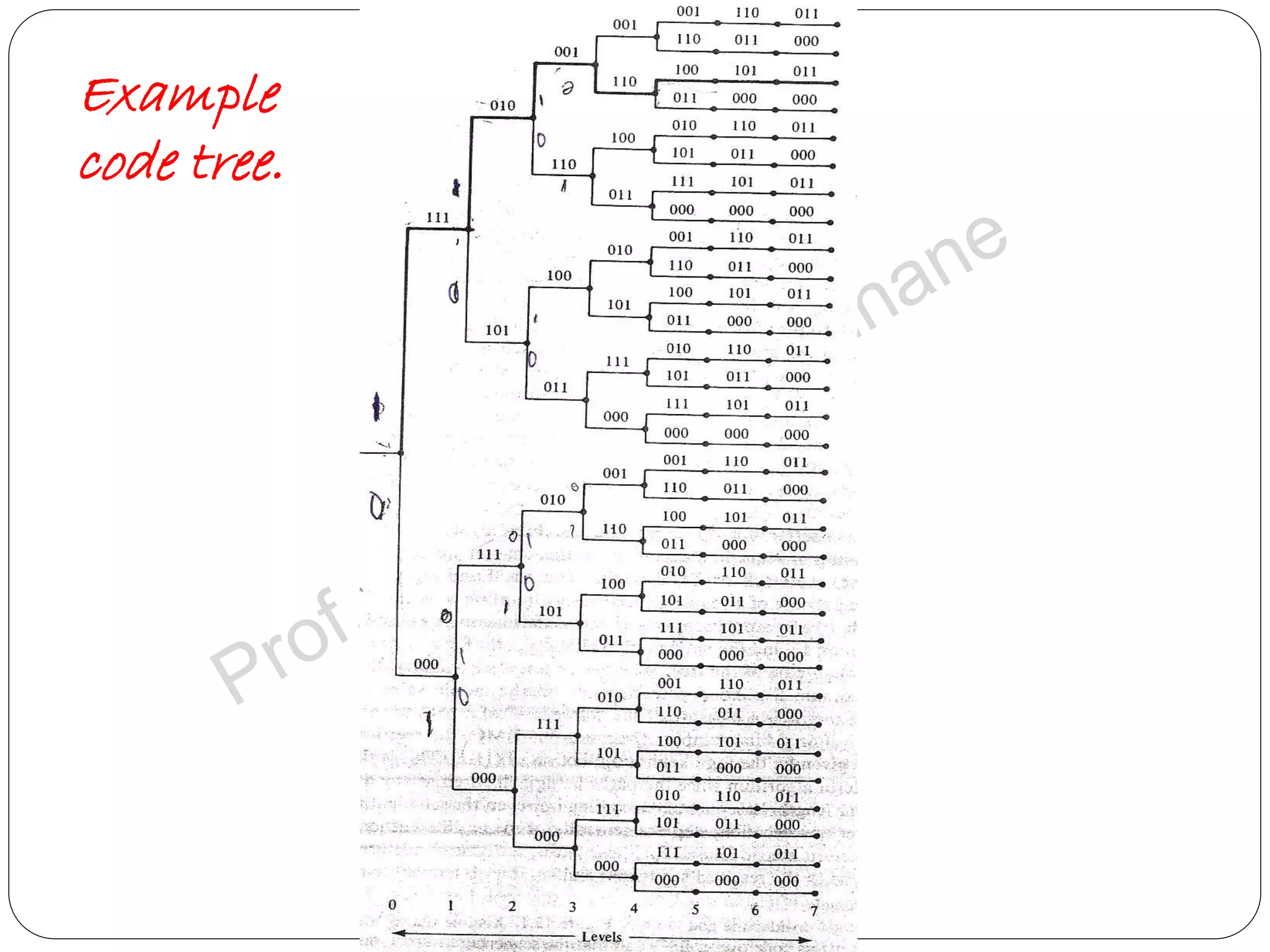
![The Stack Algorithm – ZJ Algorithm Example: (3,1,2) convolution coder has generator matrix as G(D) = [1+D, 1+D2, 1+D+D2] Let L=5. n=3, k=1, m=2 L+m+1=8 tree levels from 0 to 7. The code tree is-](https://image.slidesharecdn.com/convolutioncodes-160208053008/75/Convolution-codes-Coding-Decoding-Tree-codes-and-Trellis-codes-for-multiple-error-correction-59-2048.jpg)
![The Stack Algorithm – ZJ Algorithm For binary input and Q-ary output DMC, bit metric - M(ri|vi) = log2[P(ri|vi) / P(ri)] – R Where P(ri|vi) is channel transition probability, P(ri) is channel output symbol probability, R is code rate. The above includes length of path in metric. Partial path metric for first l branches of a path v – M([ri|vi]l-1) = ∑j=0 l-1 M(rj|vj) = ∑i=0 nl-1 M(ri|vi) Where M(rj|vj) is branch metric of jth branch and is computed by adding bit metric for the n bits on that branch. Combining above two-](https://image.slidesharecdn.com/convolutioncodes-160208053008/75/Convolution-codes-Coding-Decoding-Tree-codes-and-Trellis-codes-for-multiple-error-correction-61-2048.jpg)
![The Stack Algorithm – ZJ Algorithm M([ri|vi]l-1) = ∑i=0 nl-1 log2P(ri|vi) - ∑i=0 nl-1 P(ri) – ∑i=0 nl-1 R A binary input Q-ary out put DMC is said to be symmetric if – P(j|0) = P(Q-1-j|1), j=0,1,2…Q-1 e.g. Q=2, P(j|0) = P(1-j|1), For symmetric channel with equally likely i/p symbols, o/p symbols are also equally likely. Then- P(ri=j) = 1/Q , 0≤j≤Q-1 e.g. Q=2, P(0)=P(1)=1/2. M([ri|vi]l-1) = ∑i=0 nl-1 log2P(ri|vi) – nl log2(1/Q)– nlR = ∑i=0 nl-1 log2P(ri|vi) + nl(log2Q – R)](https://image.slidesharecdn.com/convolutioncodes-160208053008/75/Convolution-codes-Coding-Decoding-Tree-codes-and-Trellis-codes-for-multiple-error-correction-62-2048.jpg)
![The Stack Algorithm – ZJ Algorithm M([ri|vi]l-1)= ∑i=0 nl-1 log2P(ri|vi) + nl(log2Q – R) First term is metric for Viterbi algorithm. Second term represents a positive bias (Q≥2, R≤1), which increases linearly with path length. Hence longer paths with larger bias are closer to ‘End of tree” and more likely to be Maximum Likelihood path. Called Fano Metric as first introduced by Fano.](https://image.slidesharecdn.com/convolutioncodes-160208053008/75/Convolution-codes-Coding-Decoding-Tree-codes-and-Trellis-codes-for-multiple-error-correction-63-2048.jpg)
![The Stack Algorithm – ZJ Algorithm Example: For BSC(Q=2) with transition probability p, find Fano metric for truncated codeword [v]5 and [v’]0. Also find metric if p=0.1. [v]5 is shown in code tree by thick line. 2 bits in error out of 18. M([r|v]5)= 16log2(1-p) + 2log2p + 18( 1-1/3 ) = 16log2(1-p) + 2log2p + 12 M([r|v’]0)= 2log2(1-p) + log2p + 3( 1-1/3 ) = 2log2(1-p) + log2p + 2 If p=0.1, M([r|v]5)= 2.92 > M([r|v’]0)= -1.63](https://image.slidesharecdn.com/convolutioncodes-160208053008/75/Convolution-codes-Coding-Decoding-Tree-codes-and-Trellis-codes-for-multiple-error-correction-64-2048.jpg)
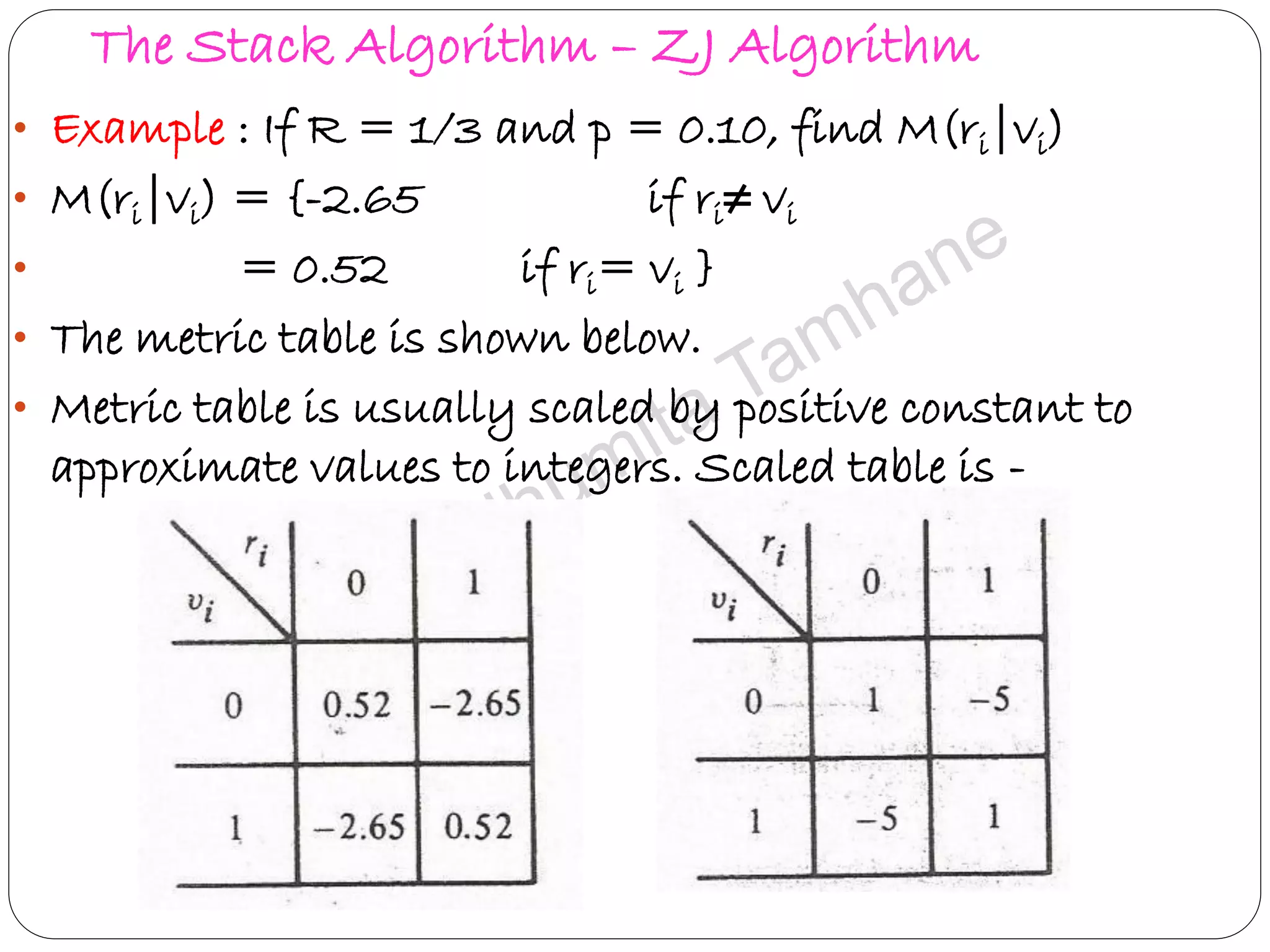
![The Stack Algorithm – ZJ Algorithm For BSC with transition probability p, the bit metrics are M(ri|vi) = log2[P(ri|vi) / P(ri)] – R = log2 P(ri|vi) - log2P(ri) – R P(ri) = ½. M(ri|vi) = log2 p- log2 2 – R M(ri|vi) = {log2 2p - R if ri≠ vi = log2 2(1-p) – R if ri= vi }](https://image.slidesharecdn.com/convolutioncodes-160208053008/75/Convolution-codes-Coding-Decoding-Tree-codes-and-Trellis-codes-for-multiple-error-correction-65-2048.jpg)

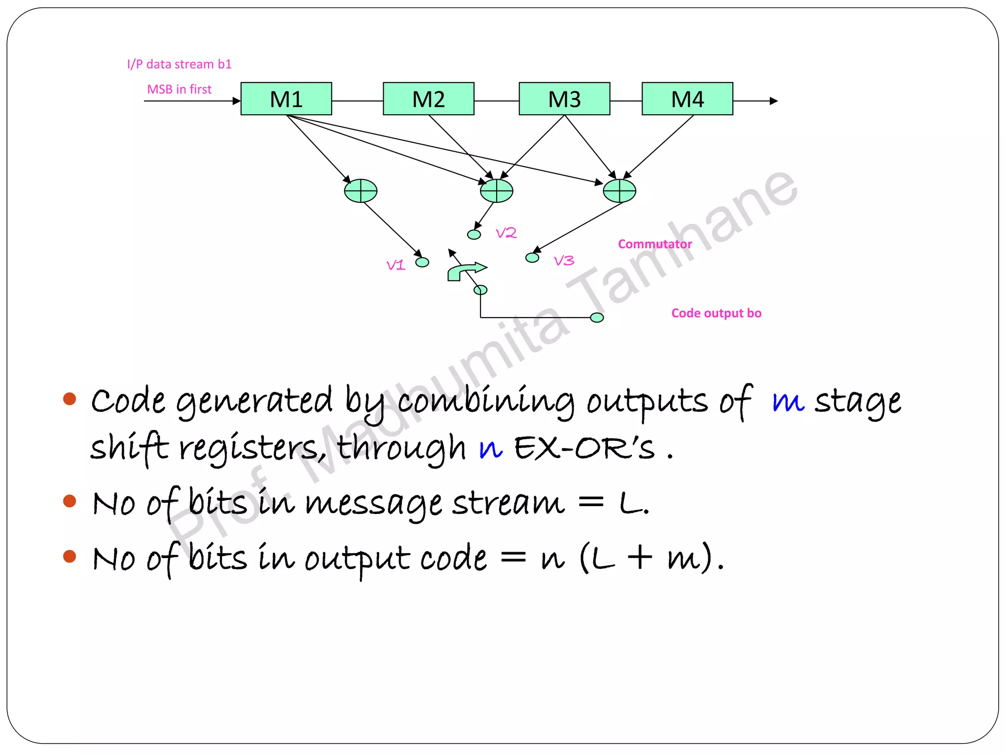
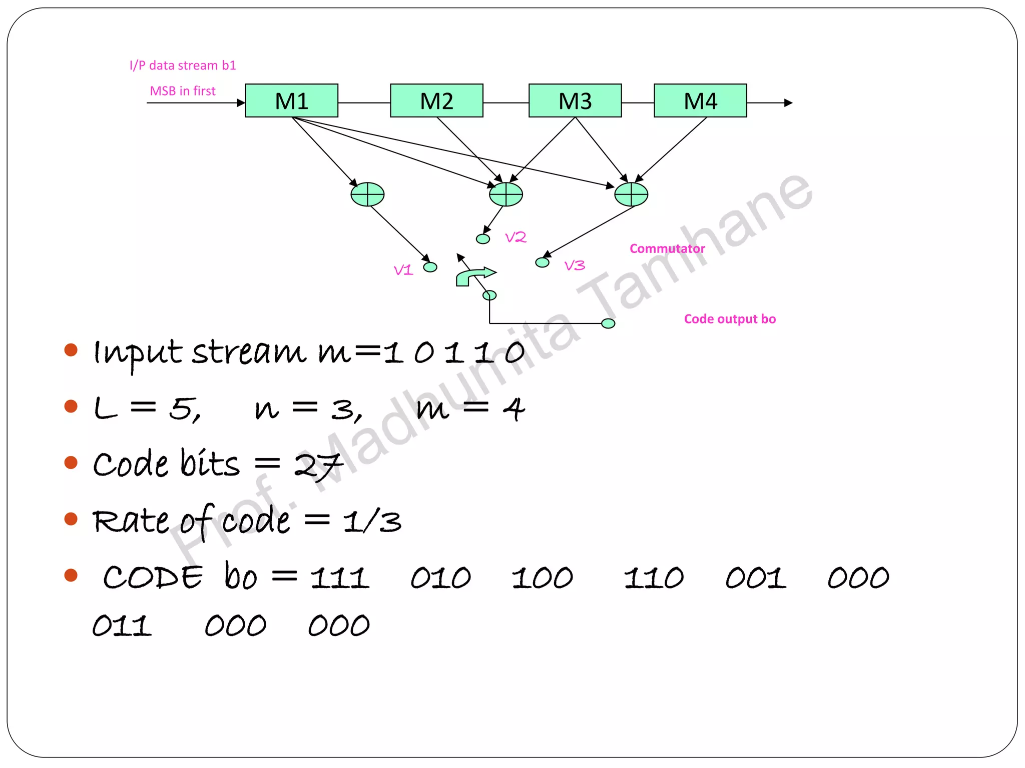
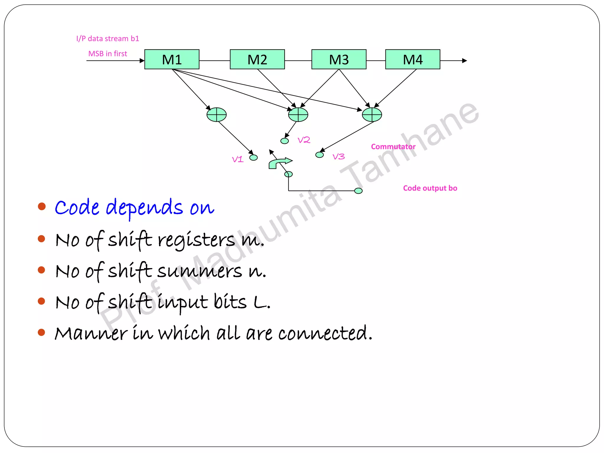
The document discusses convolution codes, detailing the differences between block and convolution codes, which are primarily used for error detection and correction, respectively. It explains the architecture of convolution encoders, including shift registers, generator polynomial matrices, and trellis diagrams. Additionally, it touches on decoding techniques such as the Viterbi algorithm and sequential decoding methods, highlighting their applications and advantages in improving data transmission reliability.
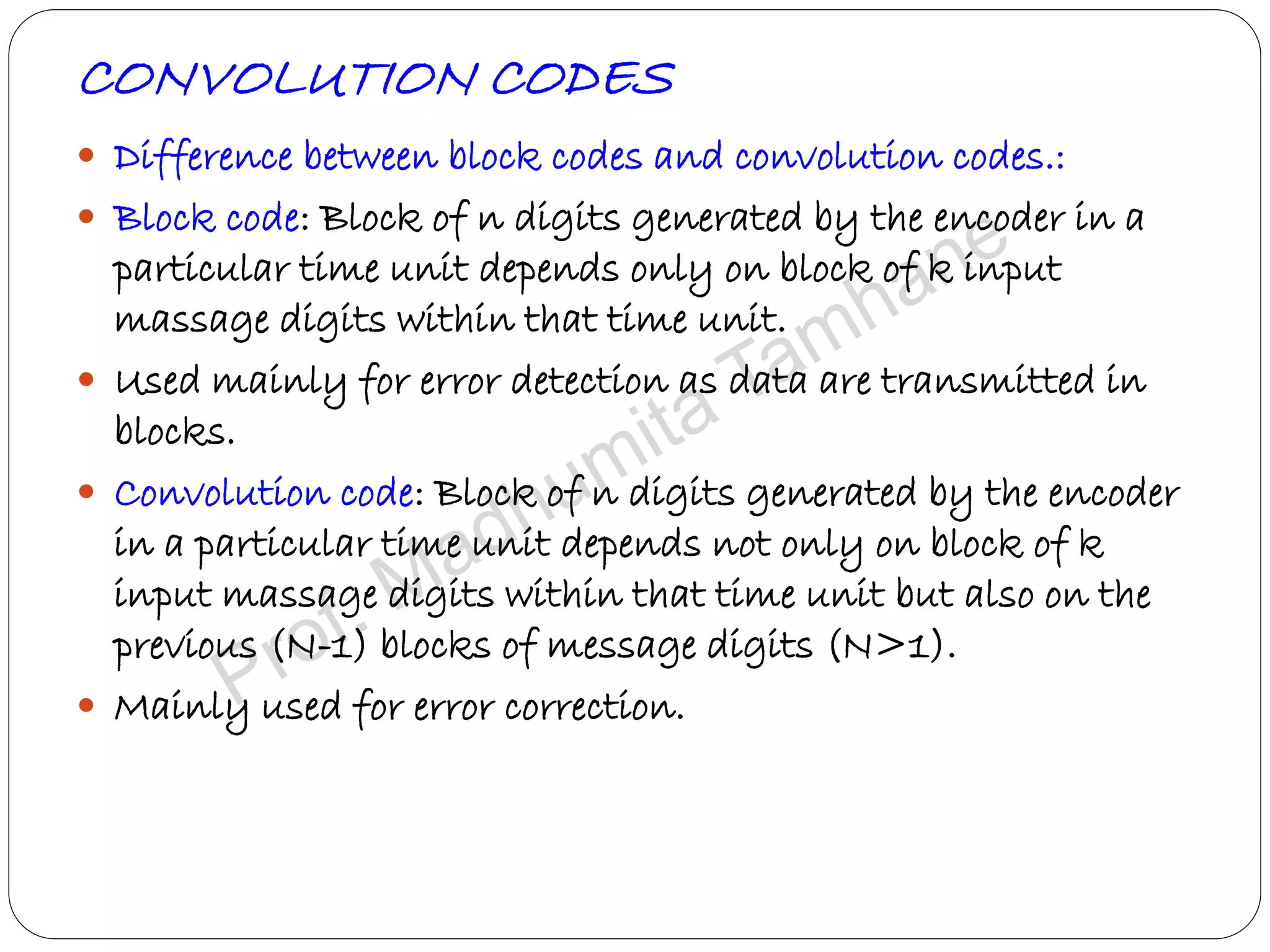
Discusses differences between block codes and convolution codes, their applications in error detection and correction.
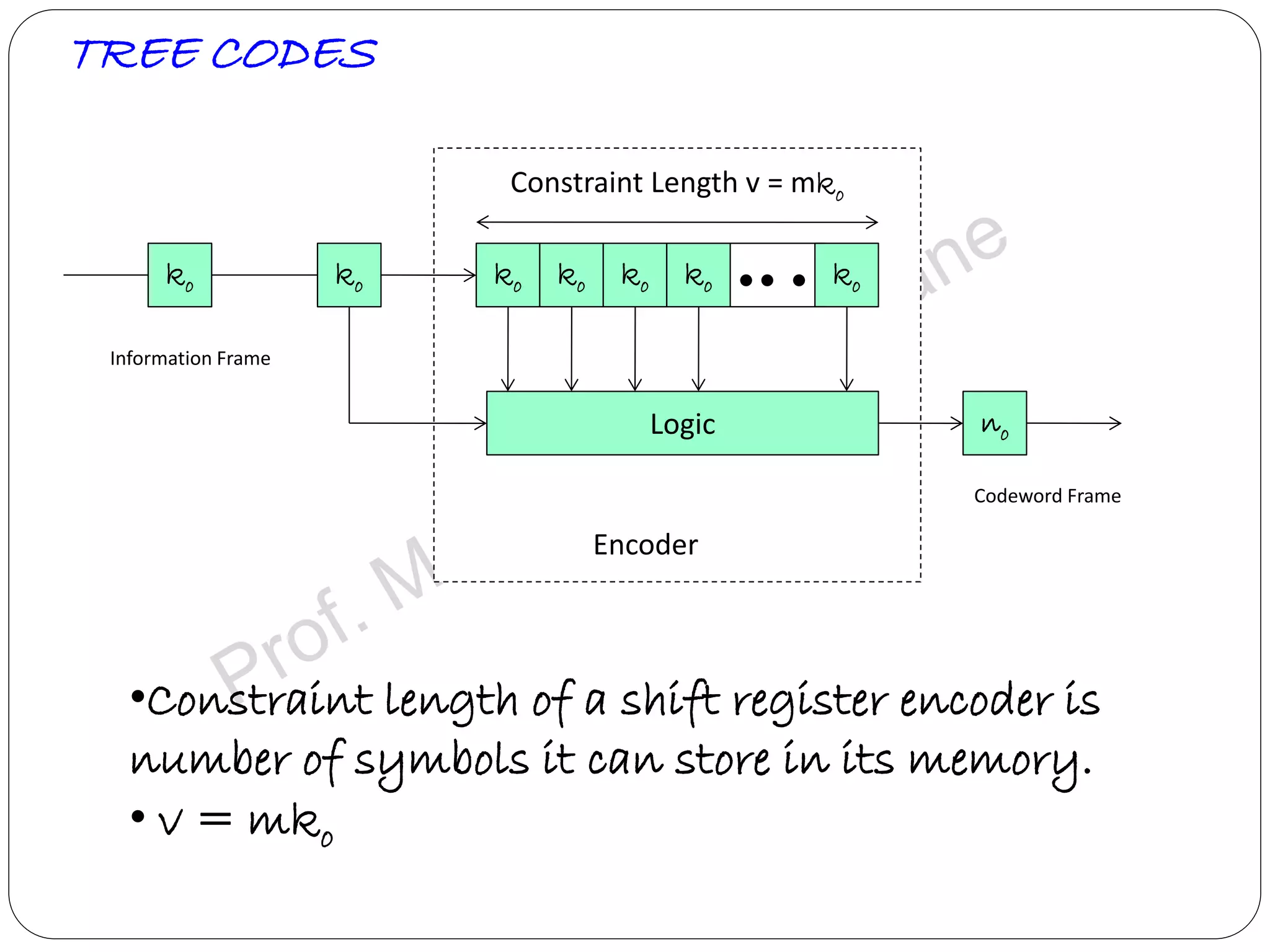
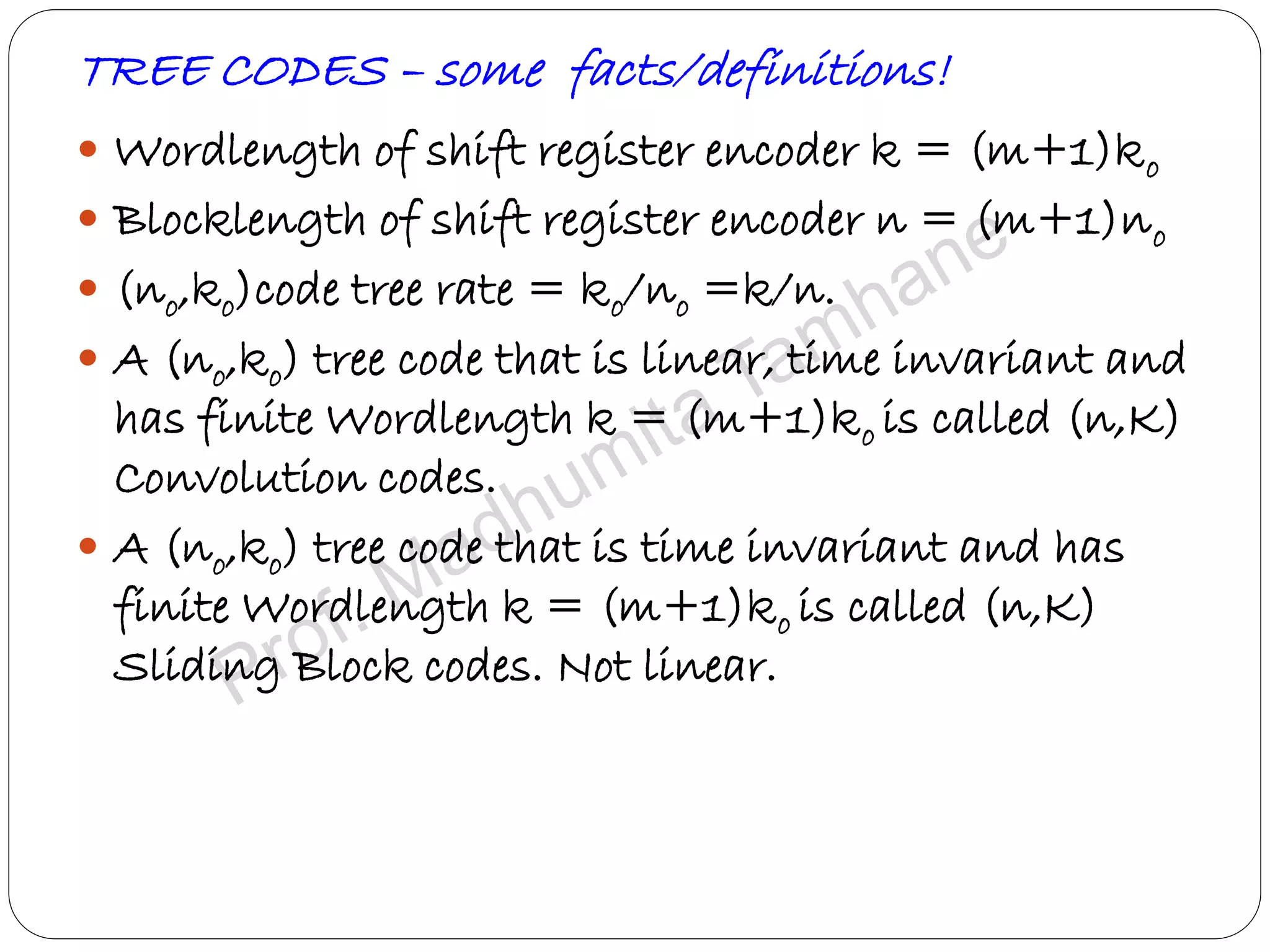
Explains tree and trellis codes, encoding logic, memory requirements, and key parameters like constraint length.
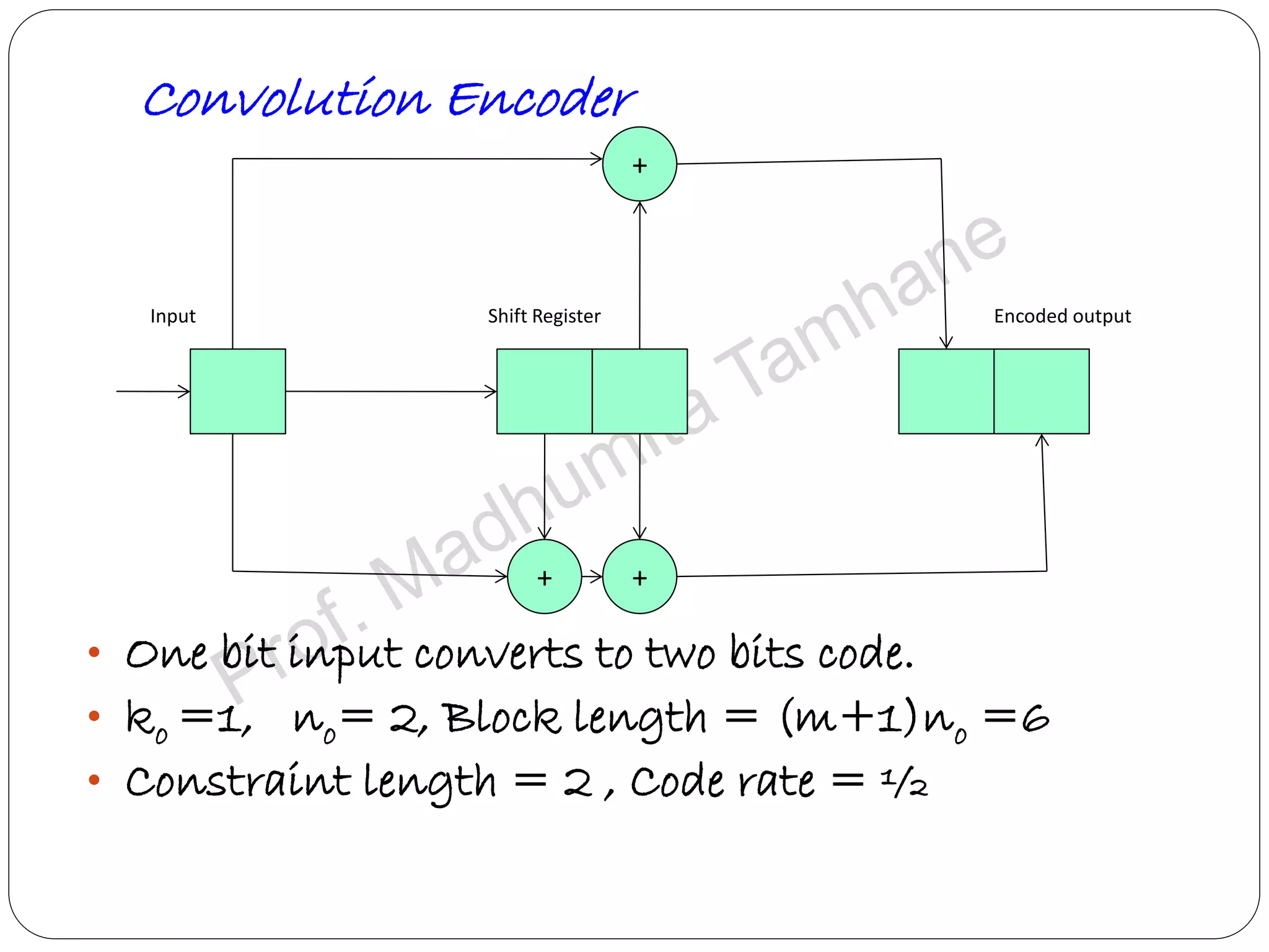
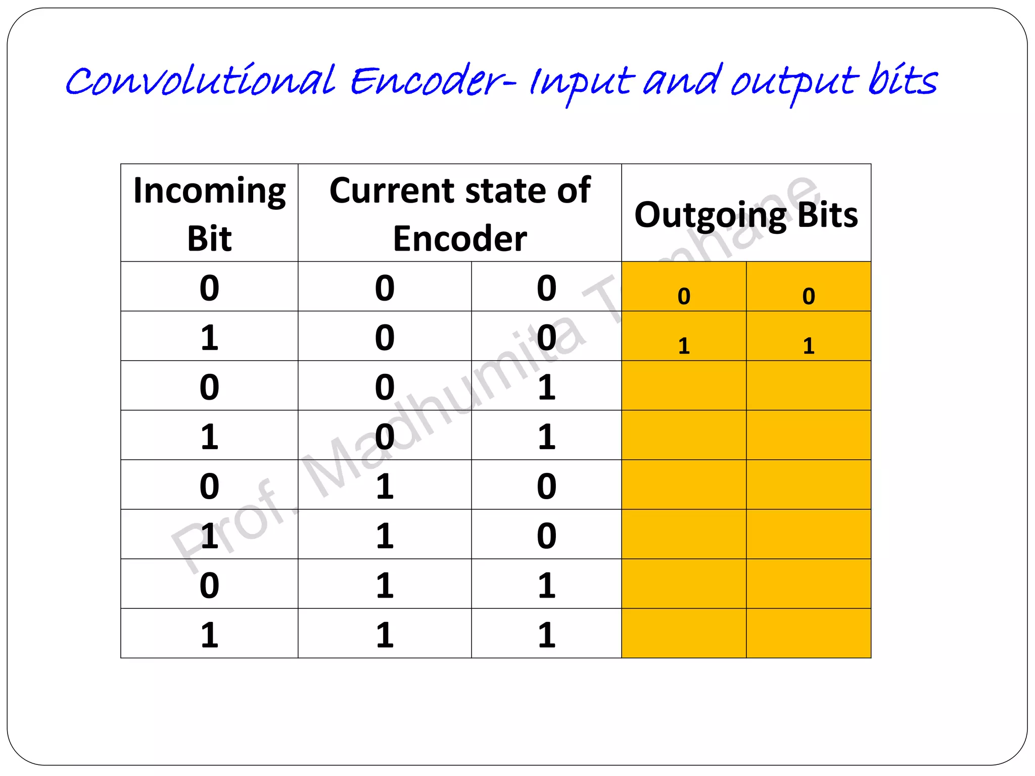
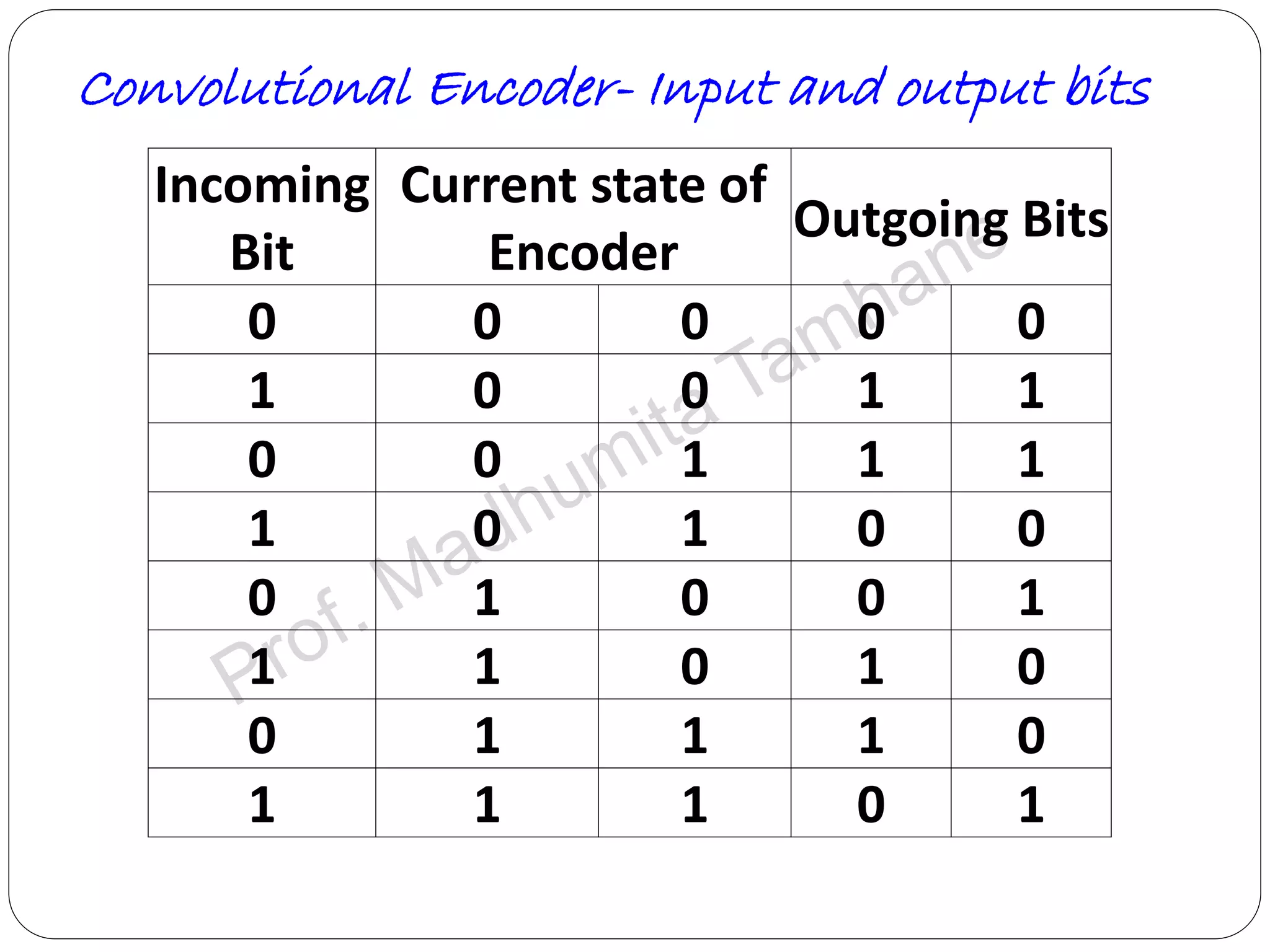
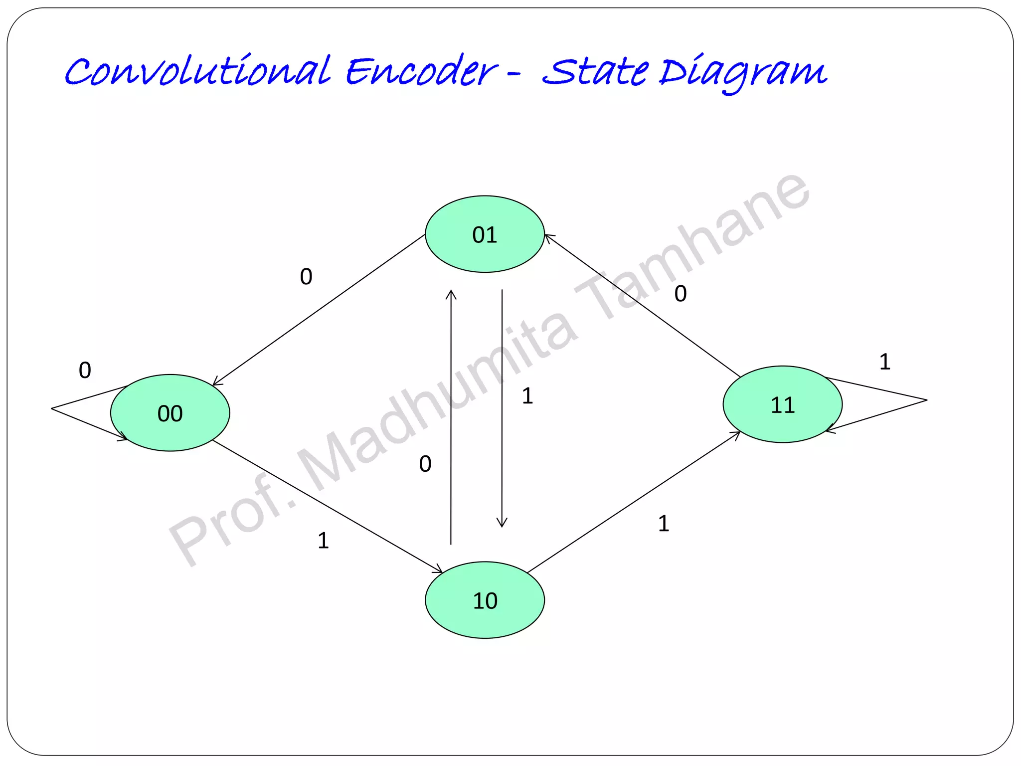
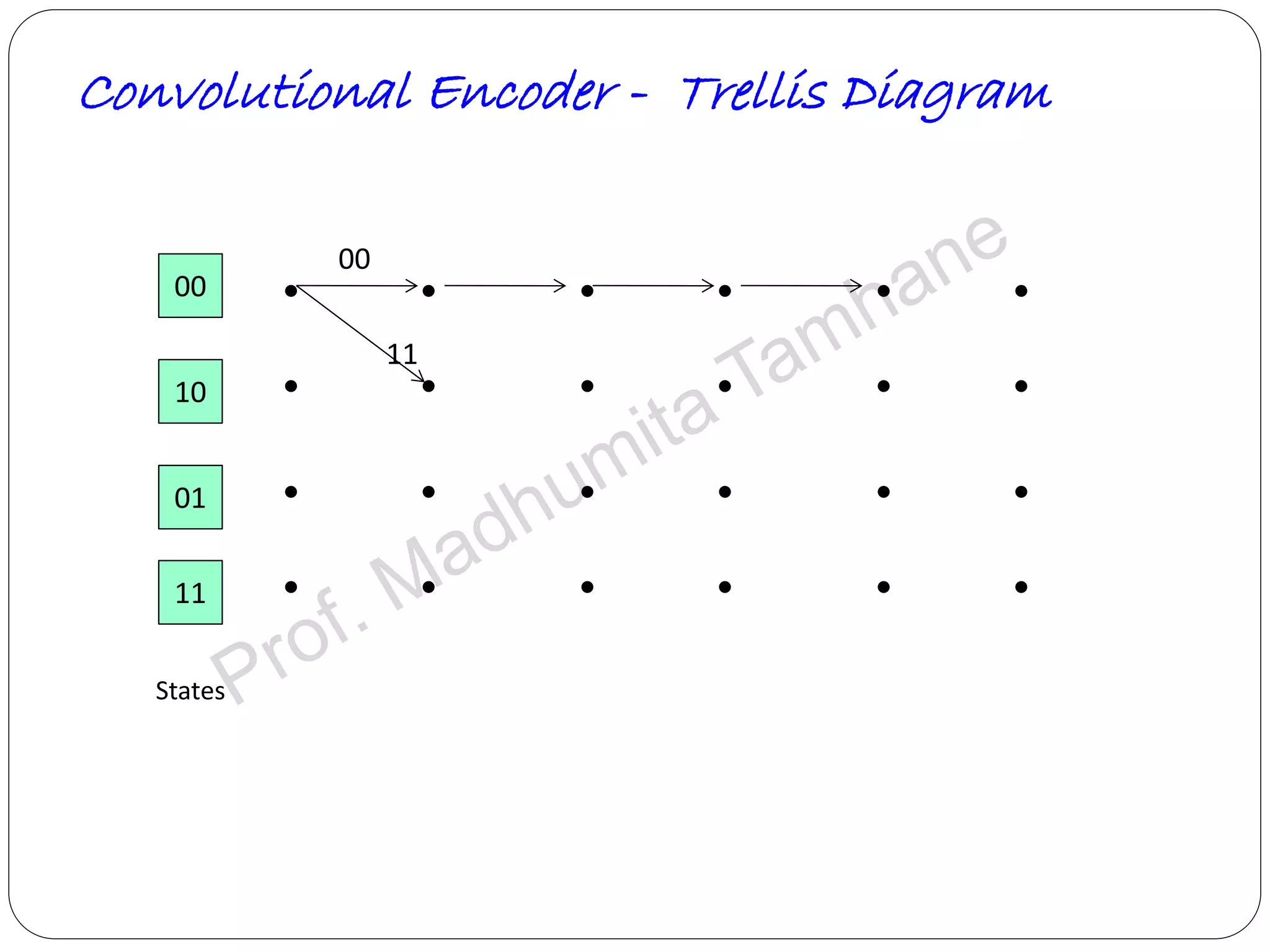
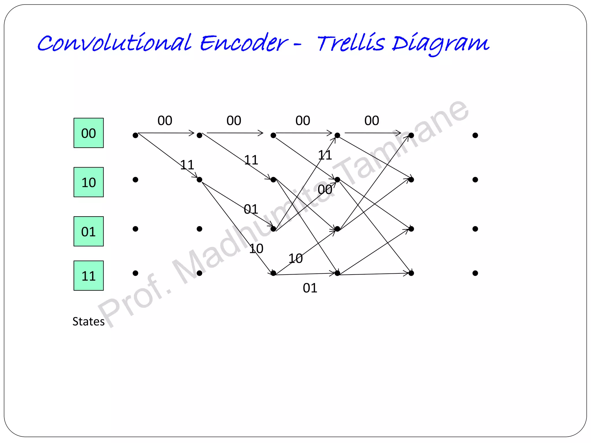
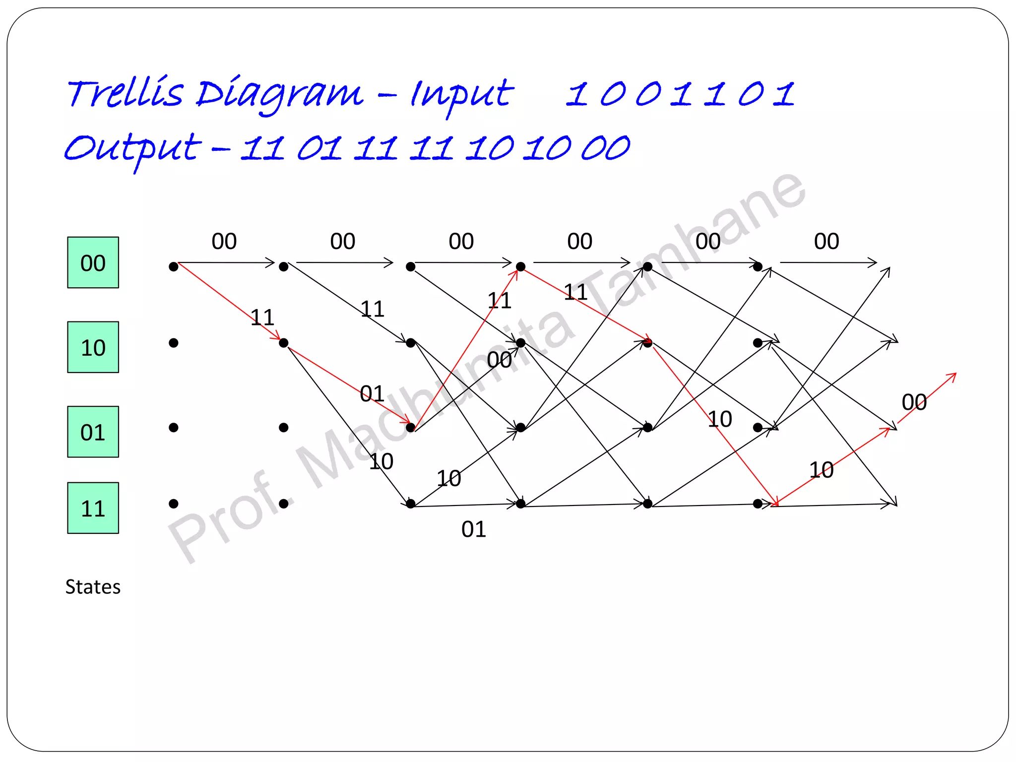
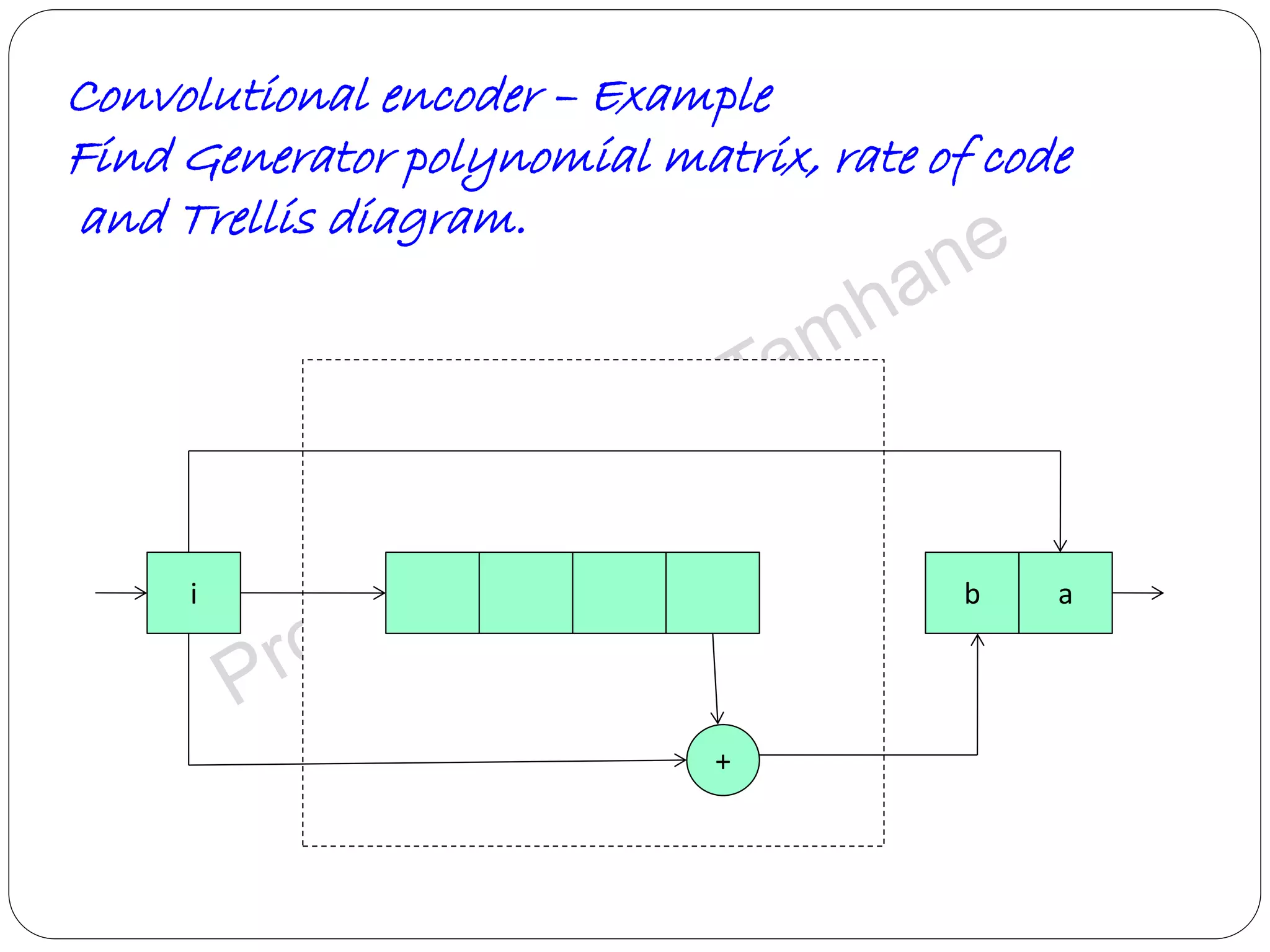
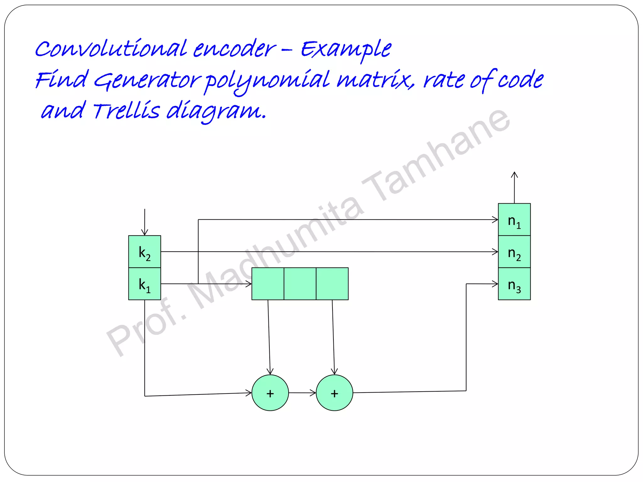
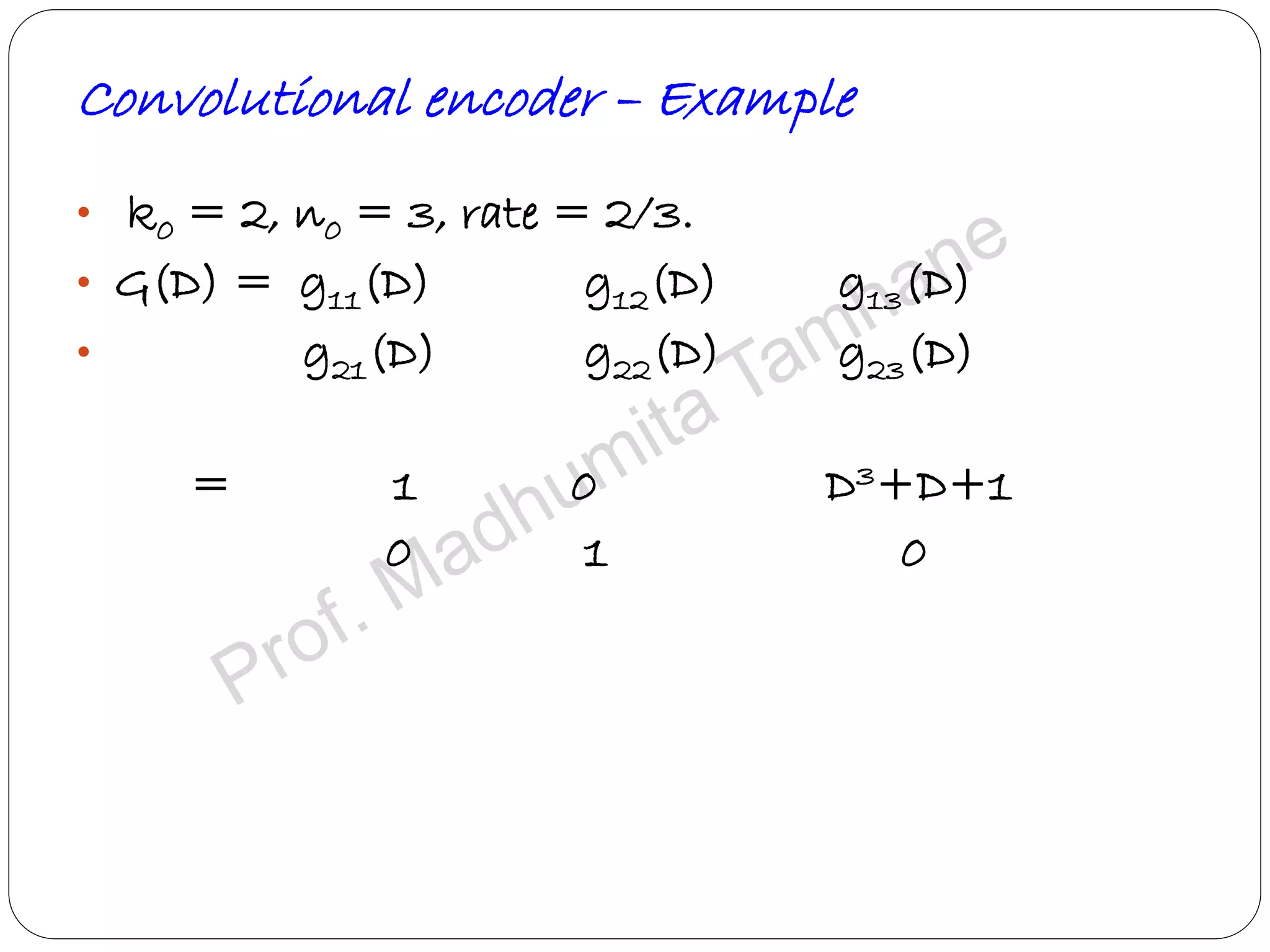
Details the structure of convolutional encoders, including input-output state diagrams and code rates.
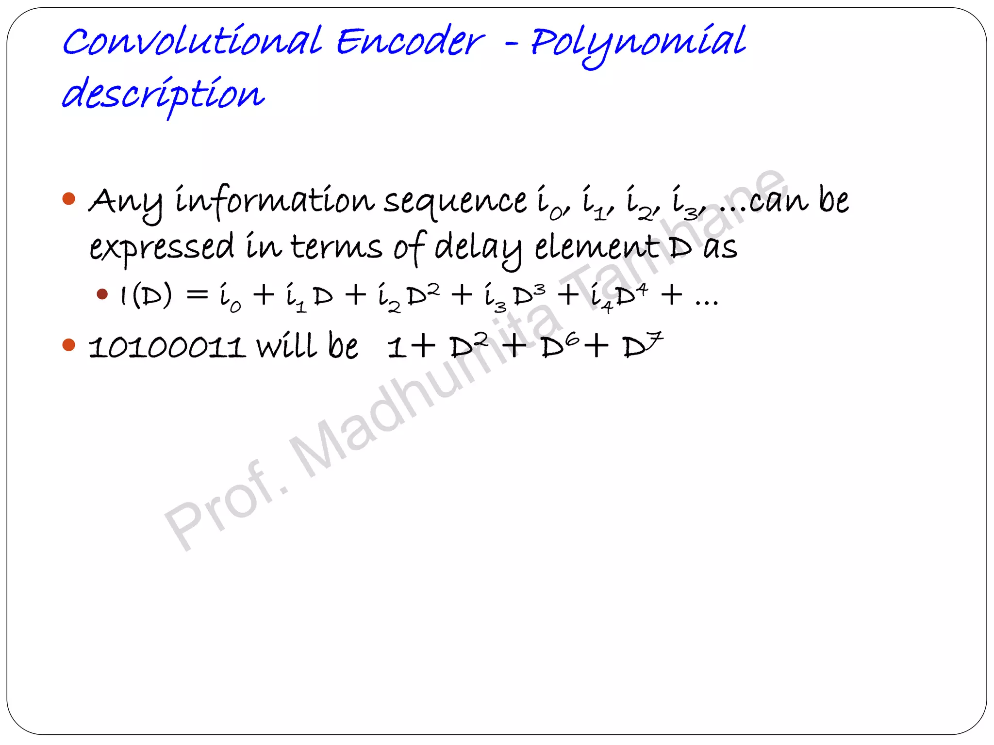
Describes polynomial representation in coding, focusing on generator polynomials and systematic encoders.
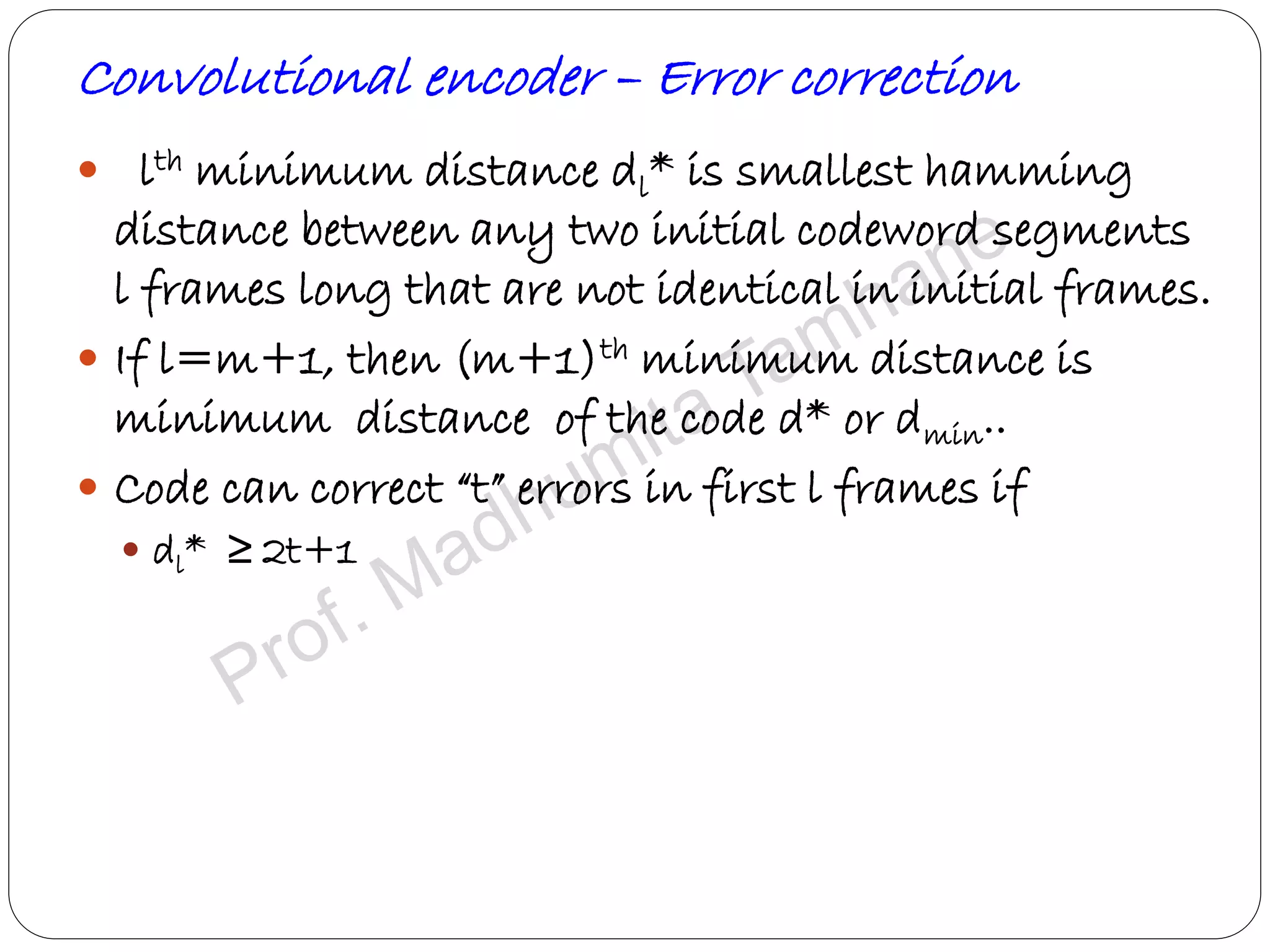
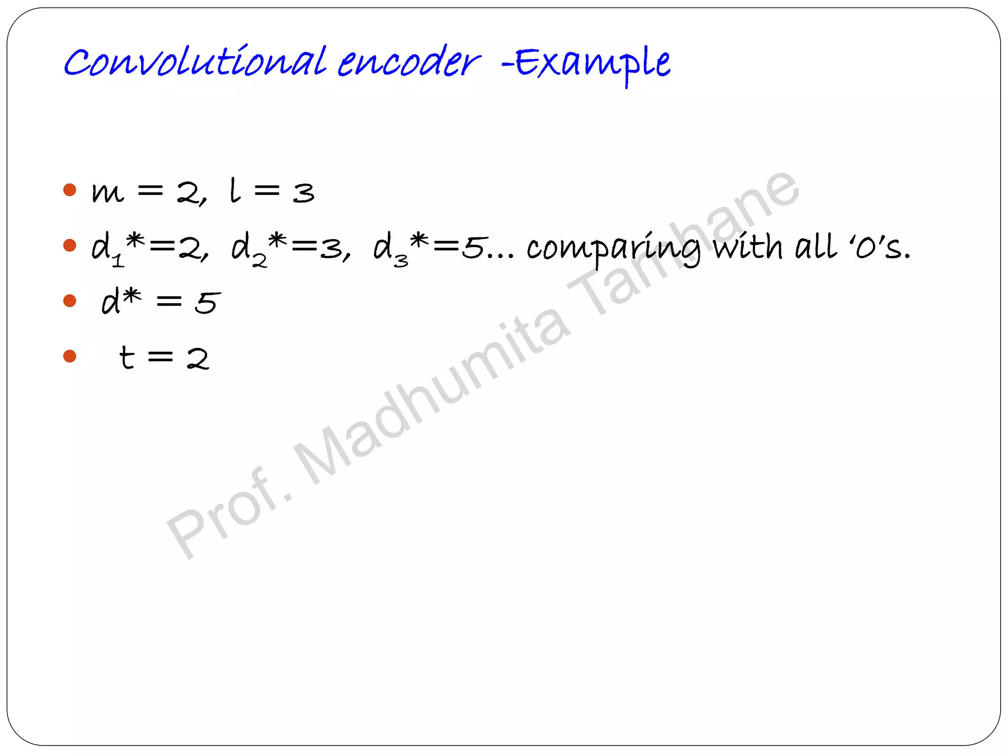
Examines minimum distance properties necessary for correcting errors in encoded data.
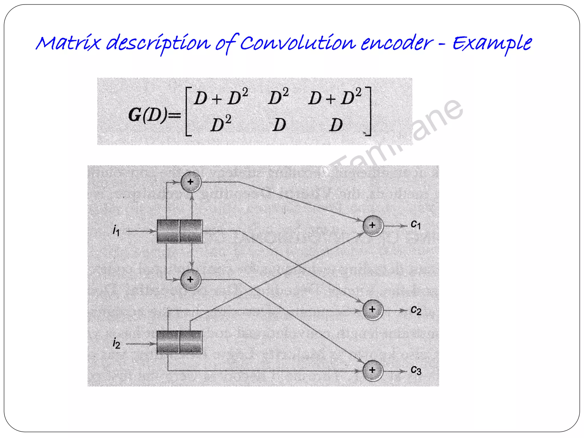
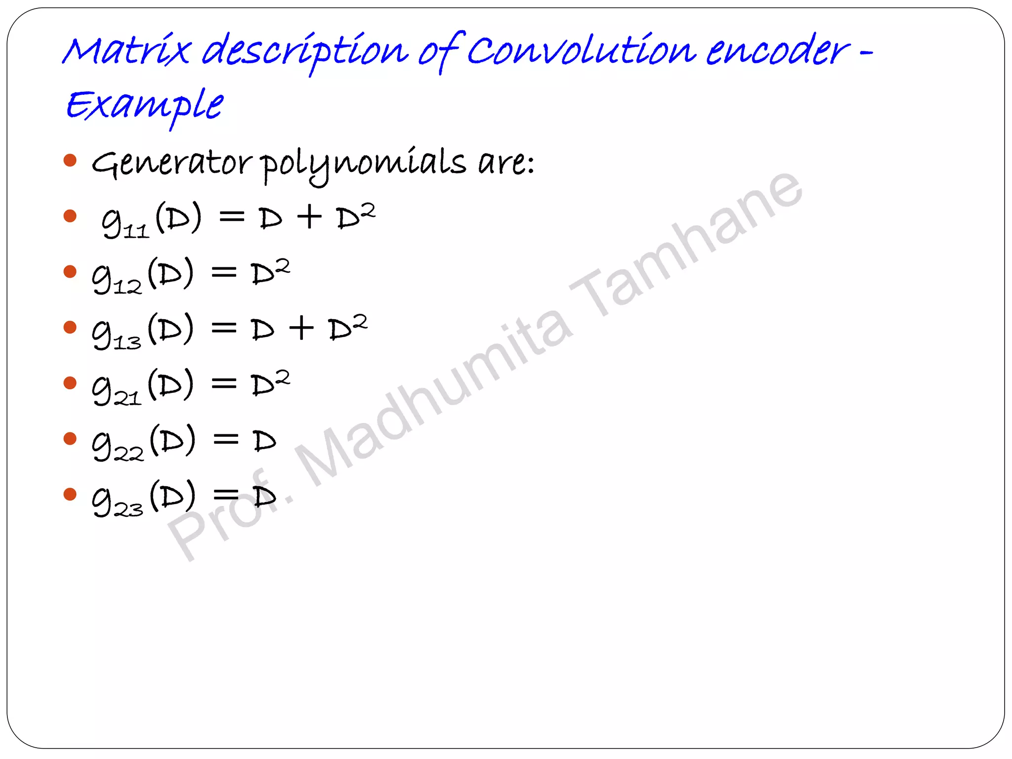
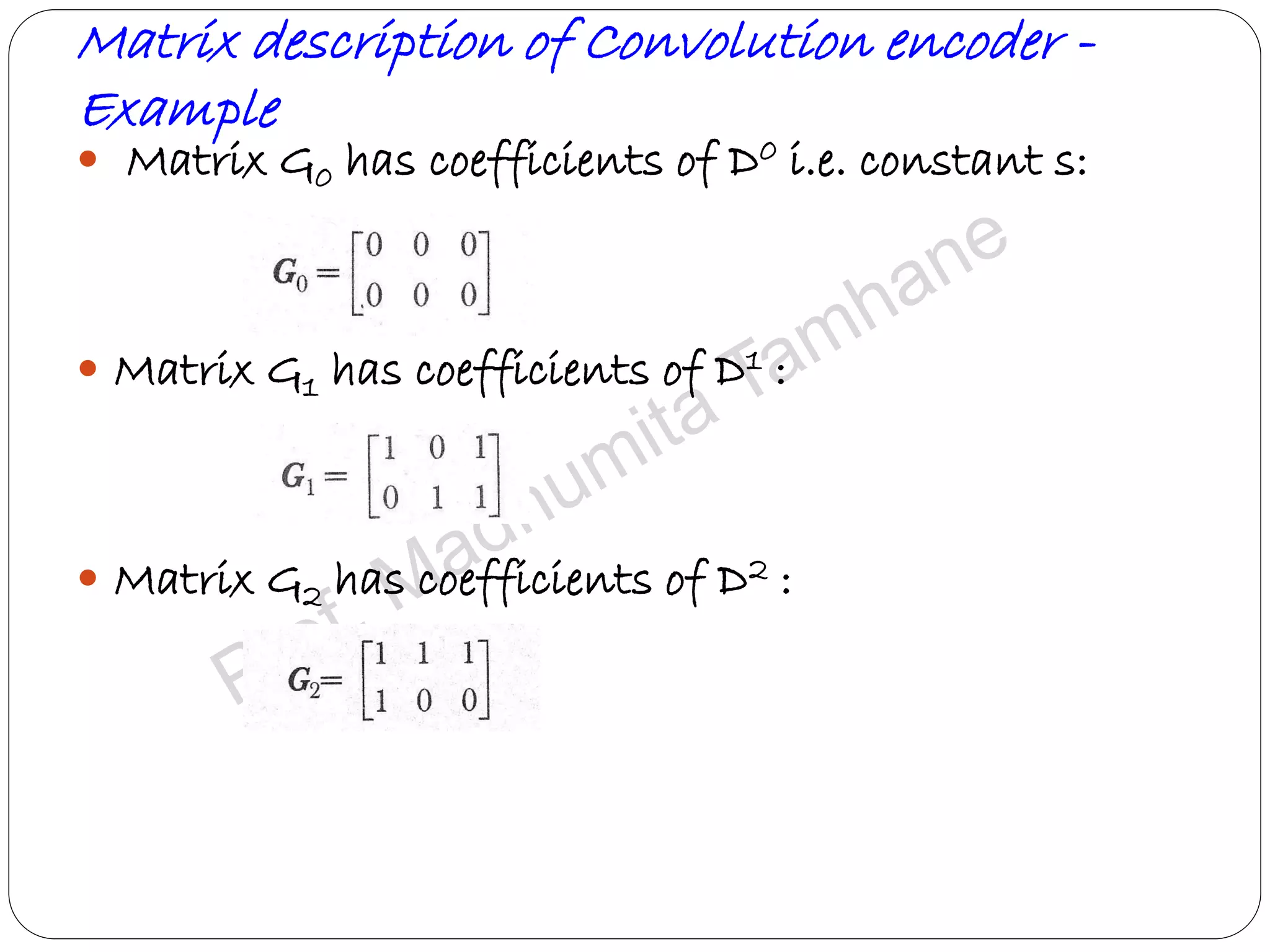
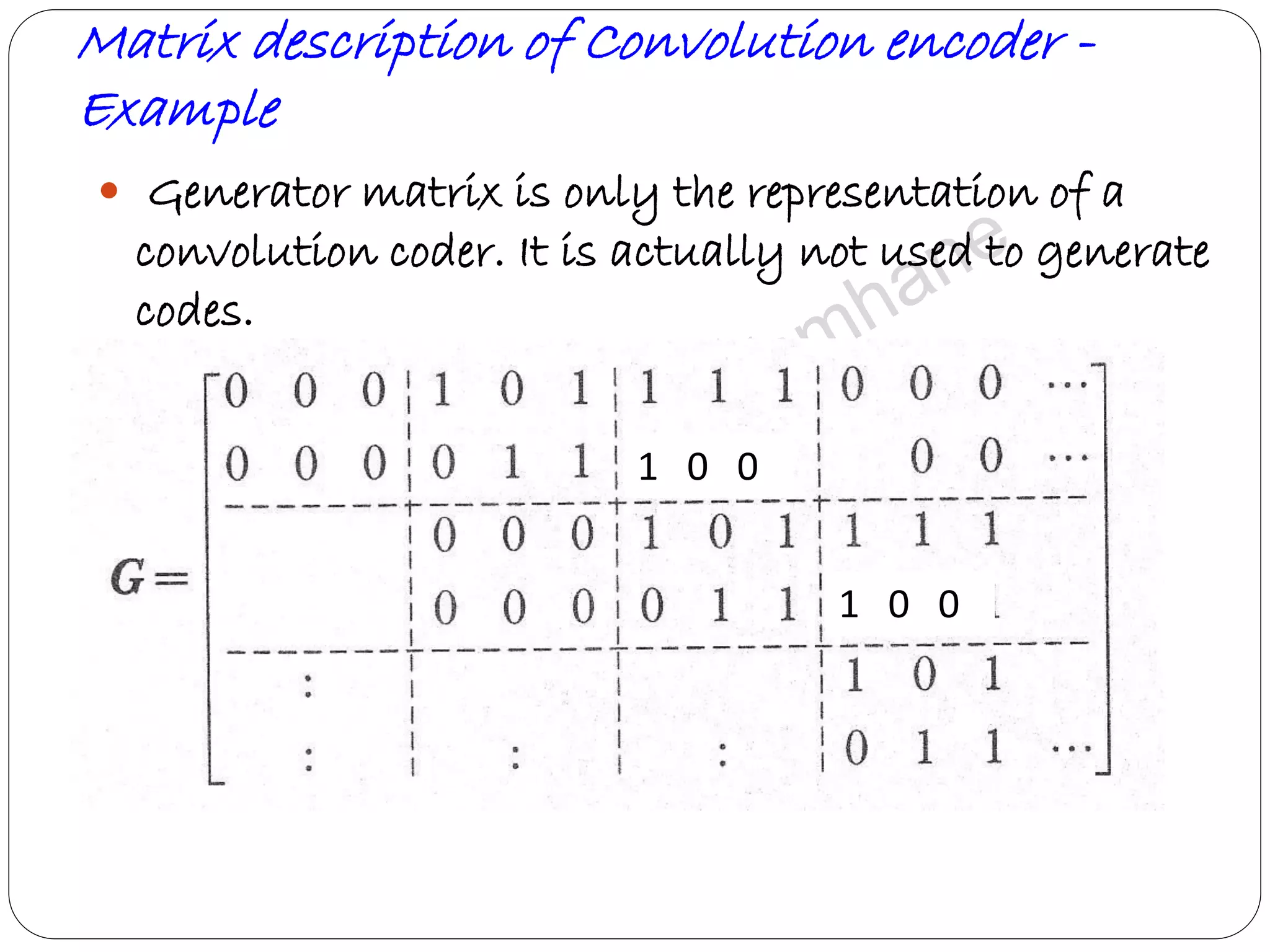
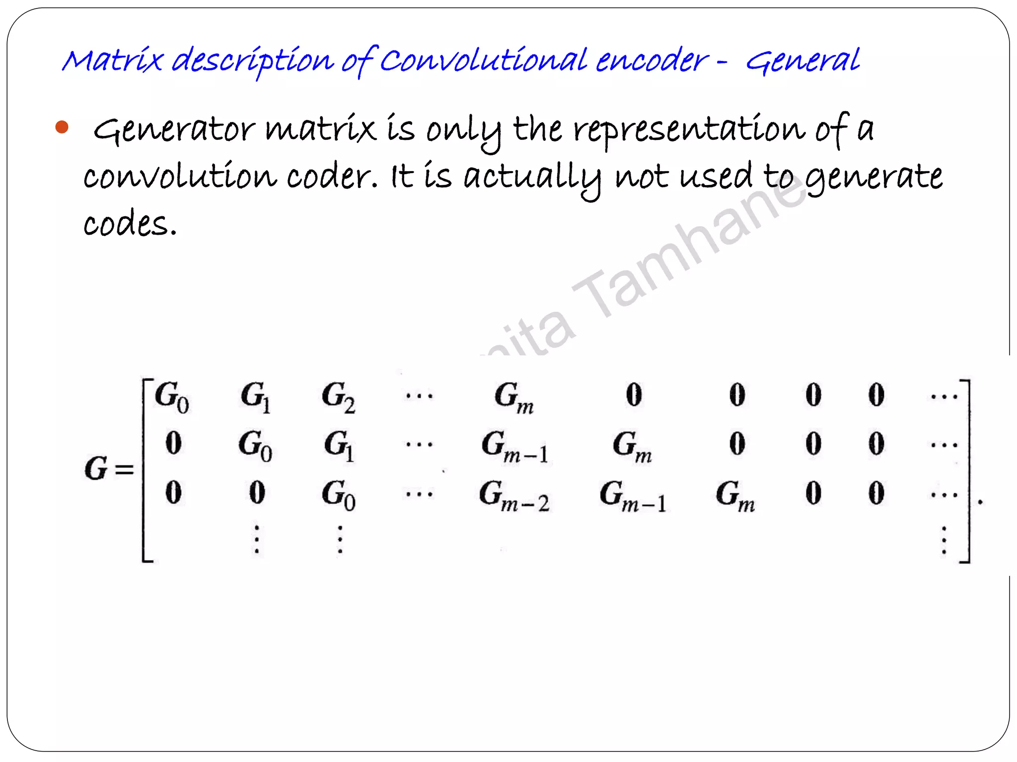
Focuses on generator matrix representation and its importance in convolution coding.
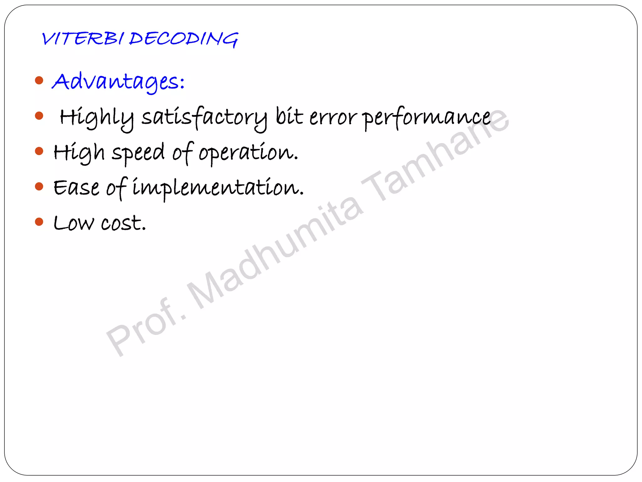
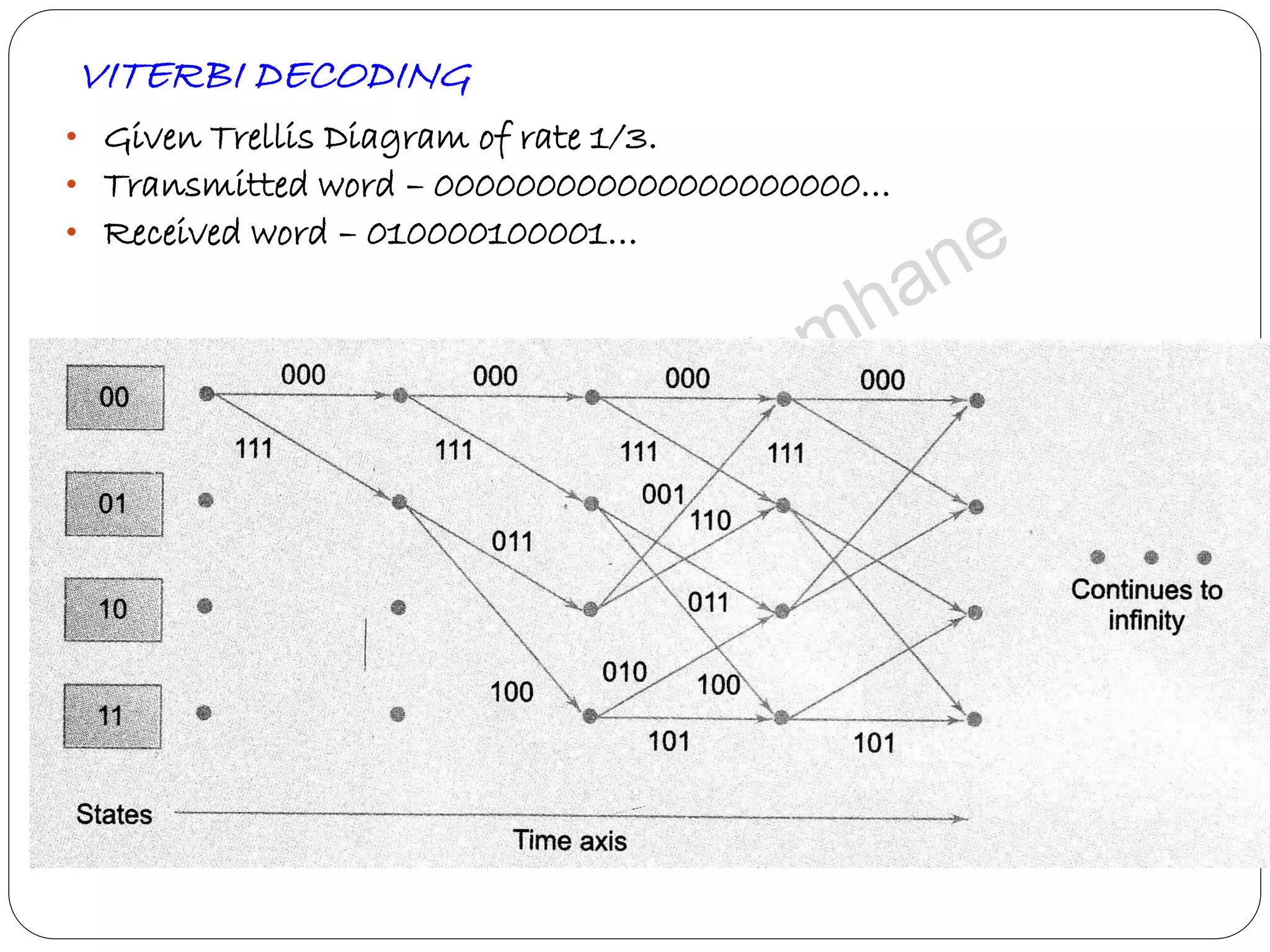
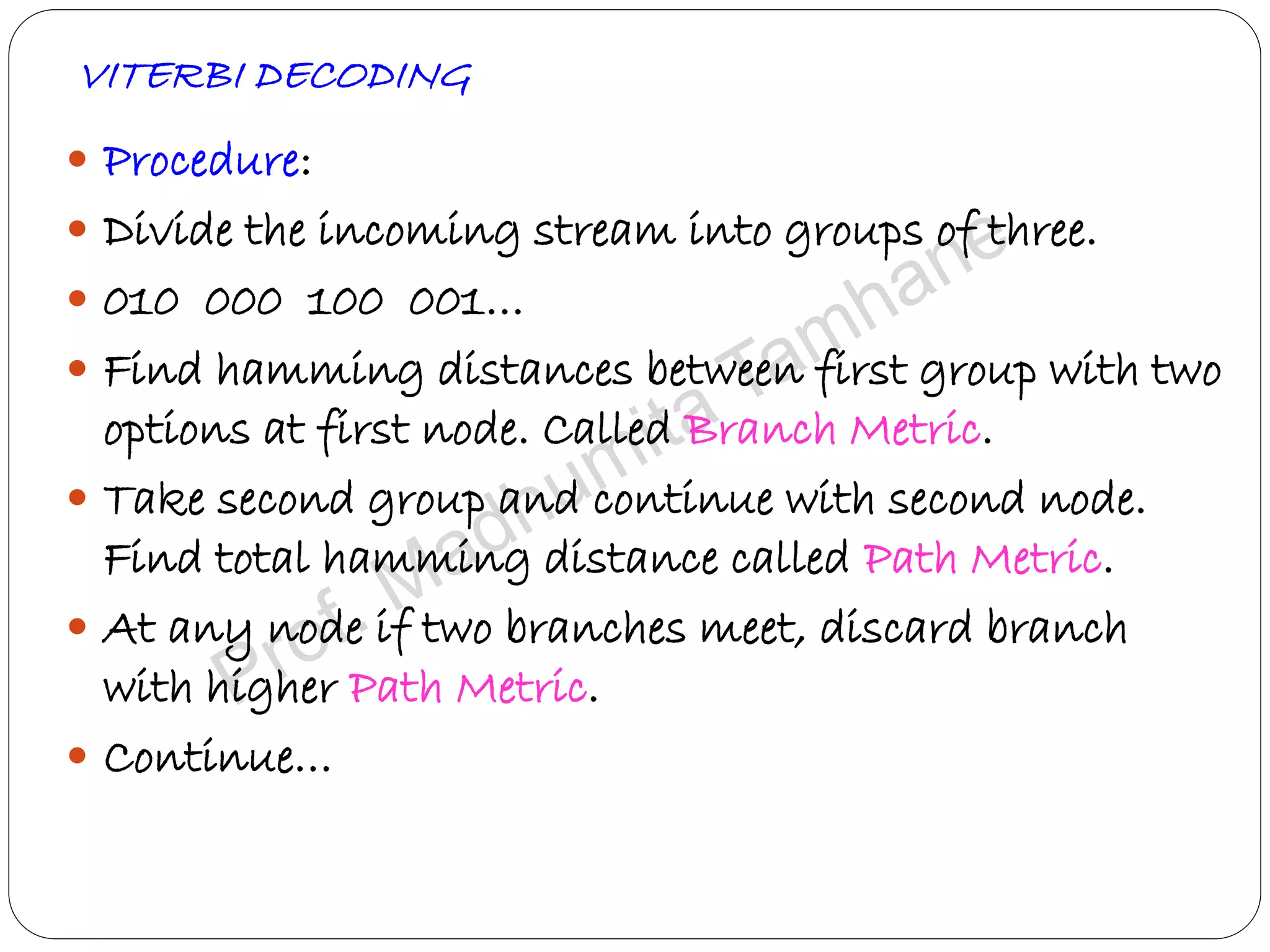
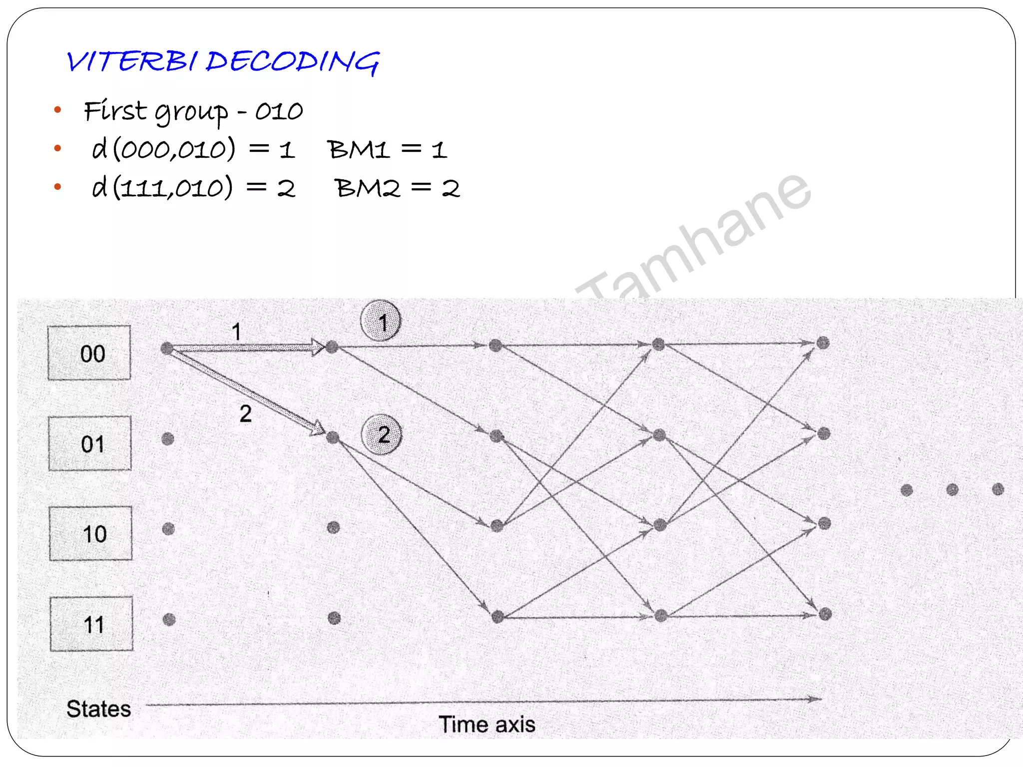
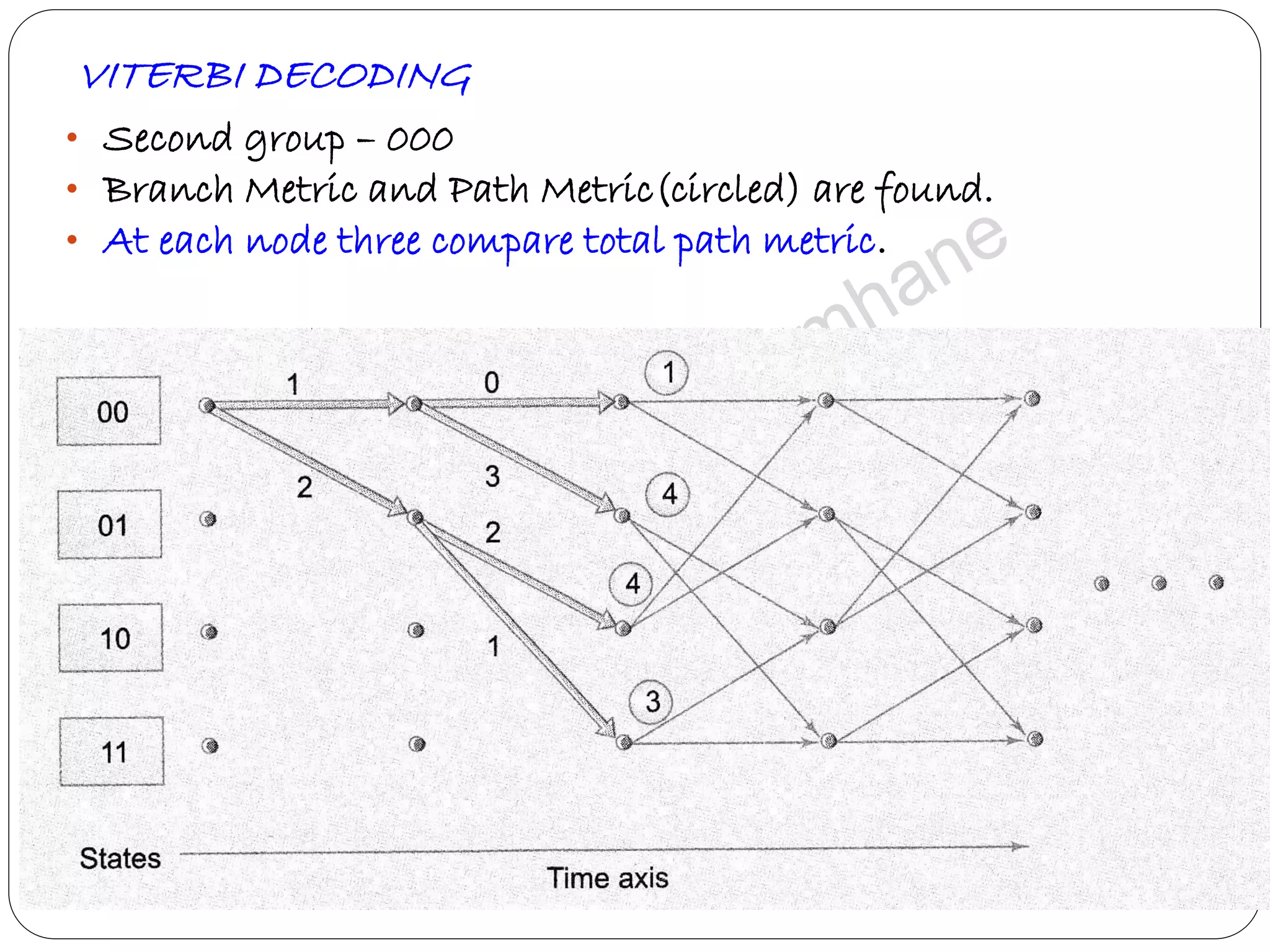
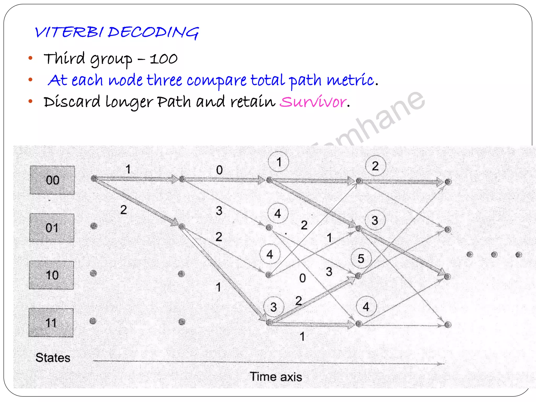
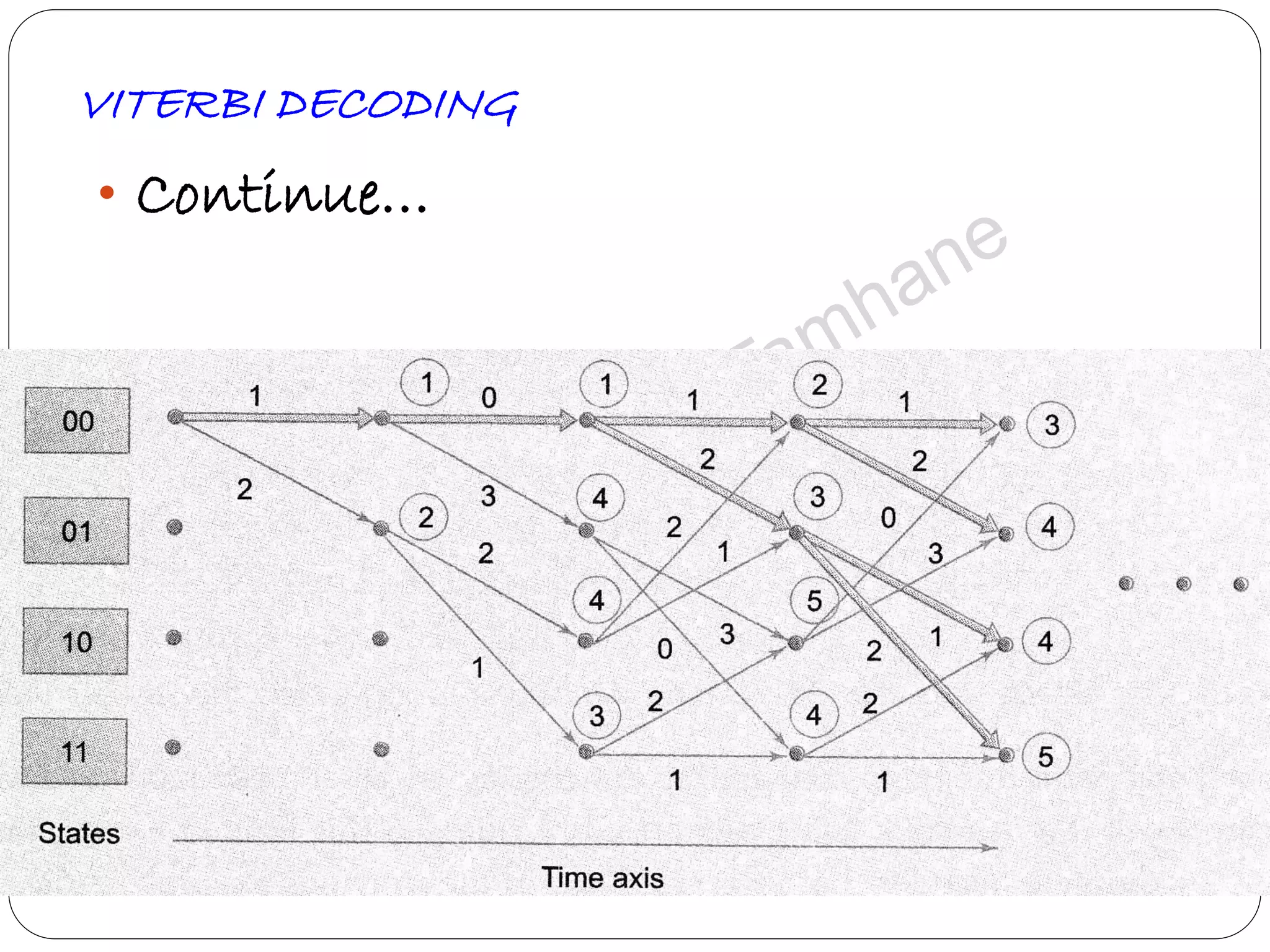
Describes Viterbi algorithm's operation, its advantages, and step-by-step decoding strategy.
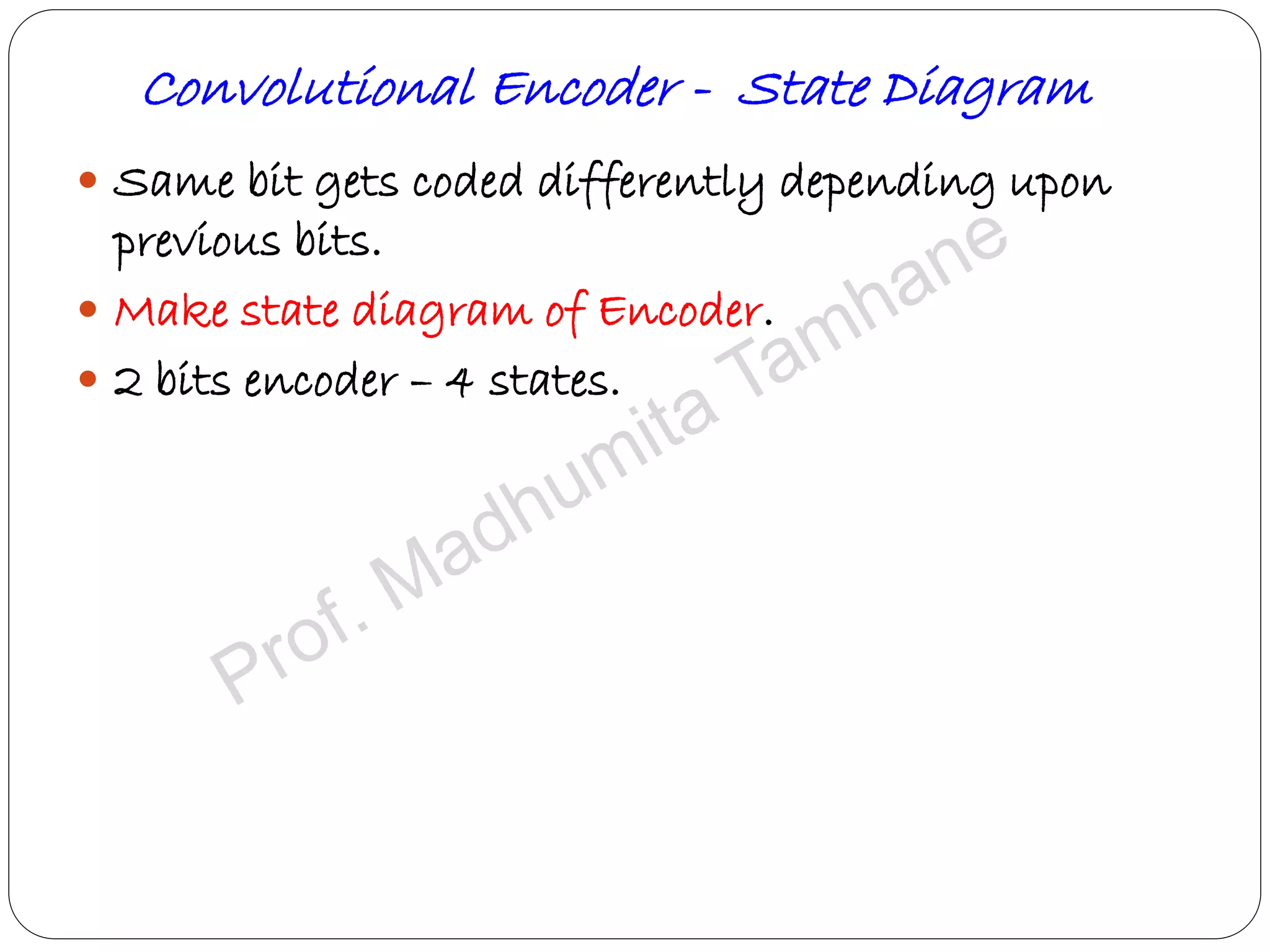
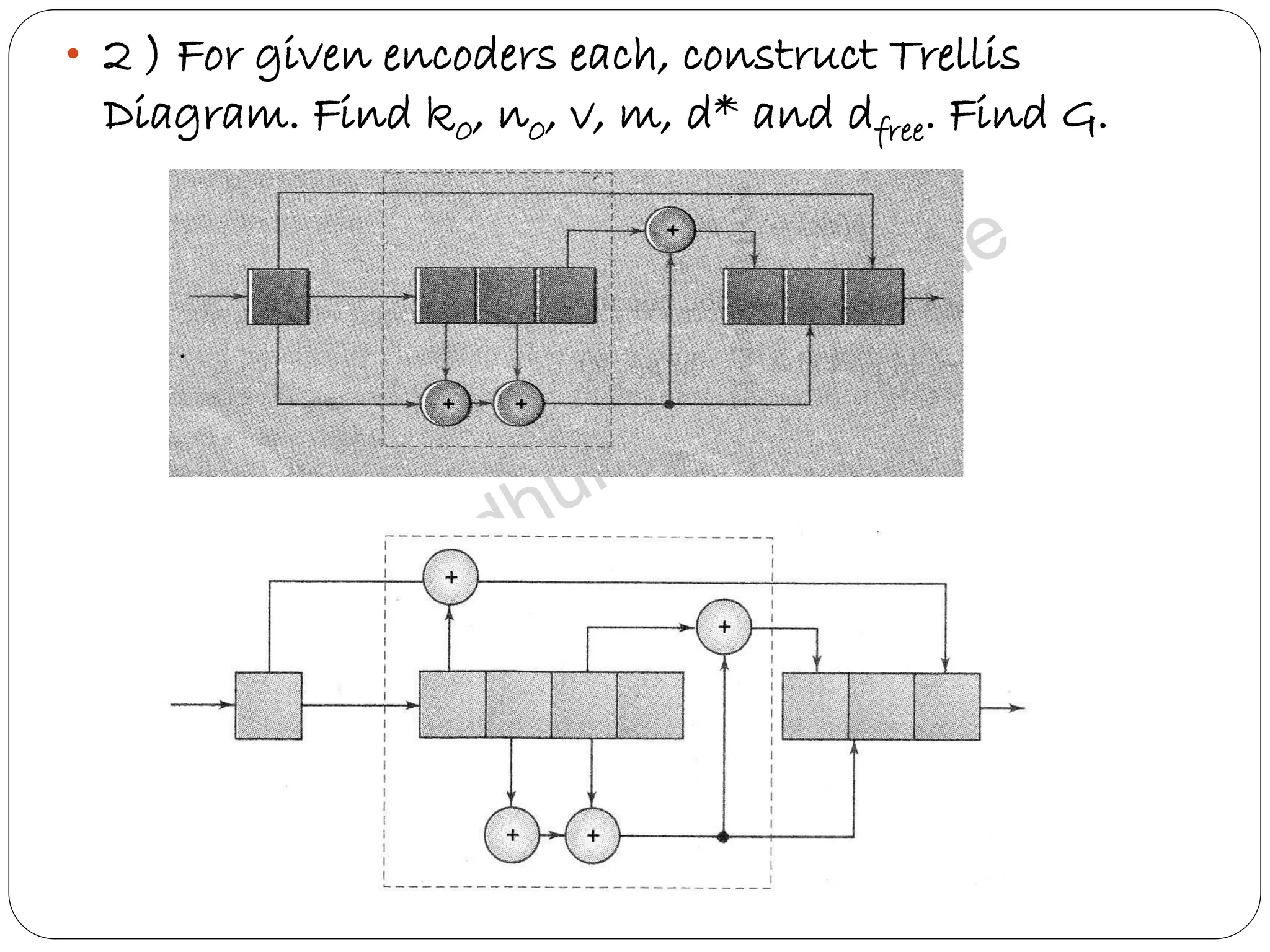
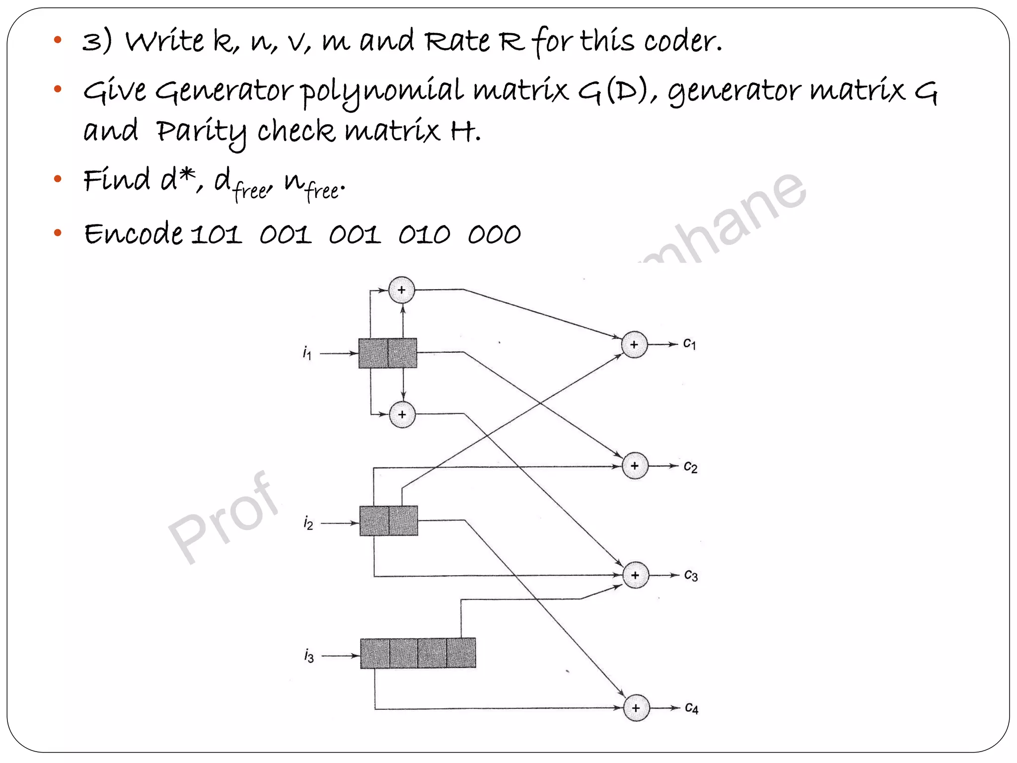
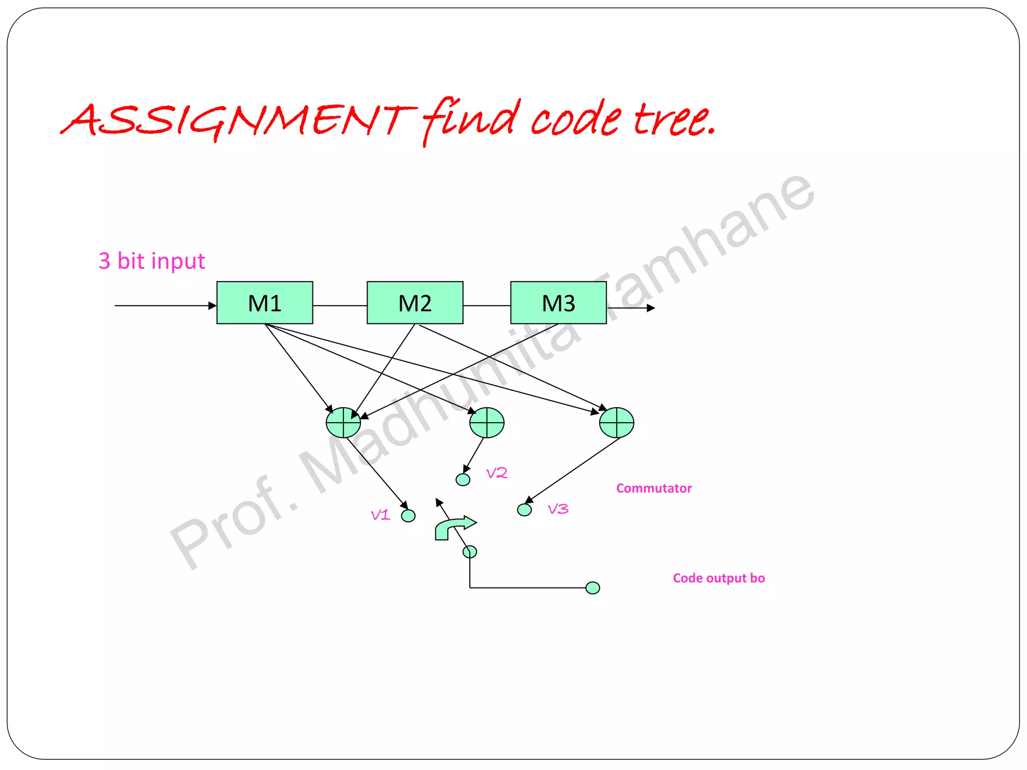
Presents assignments related to convolutional coding design, state diagram construction, and performance analysis.
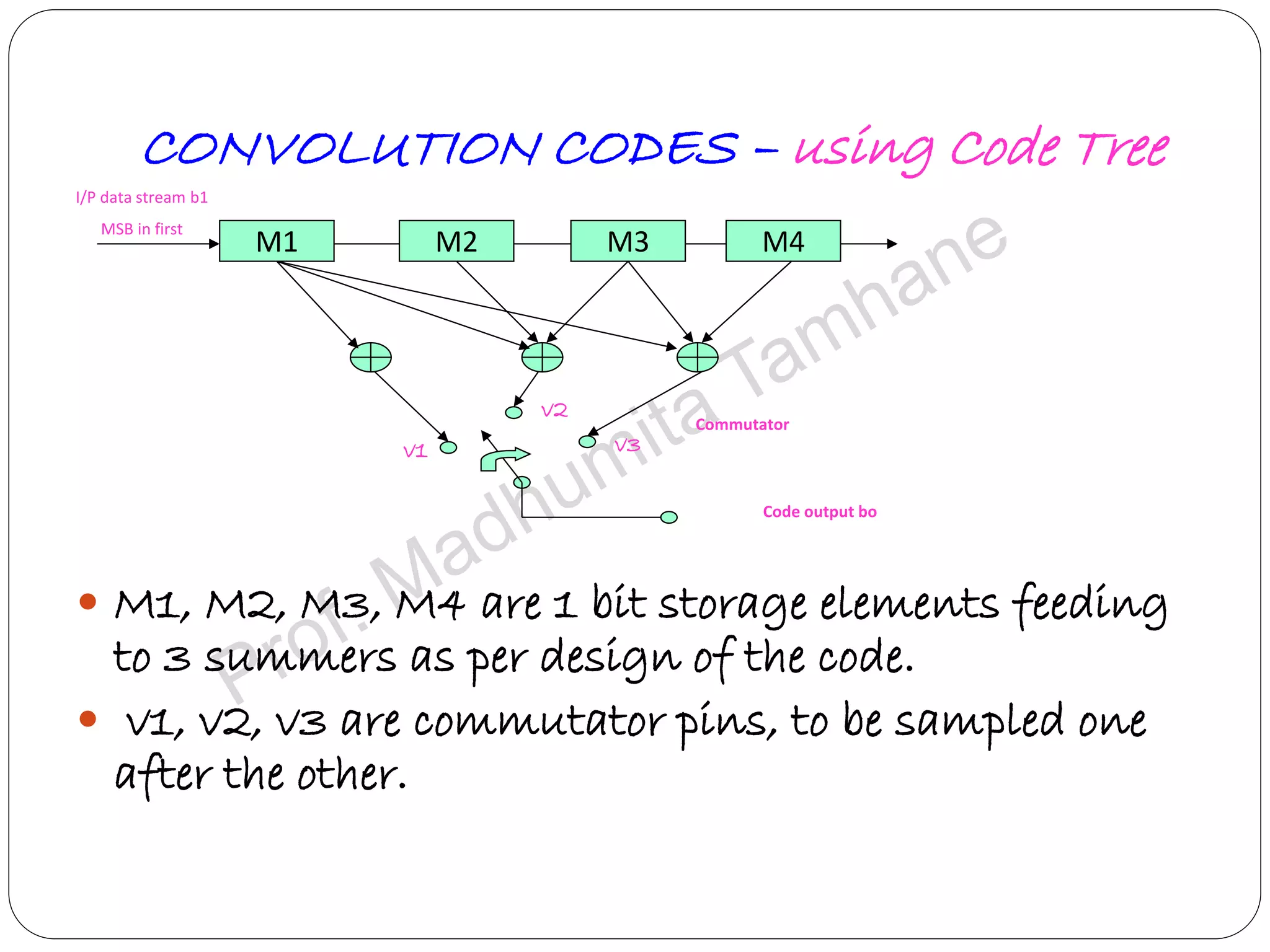
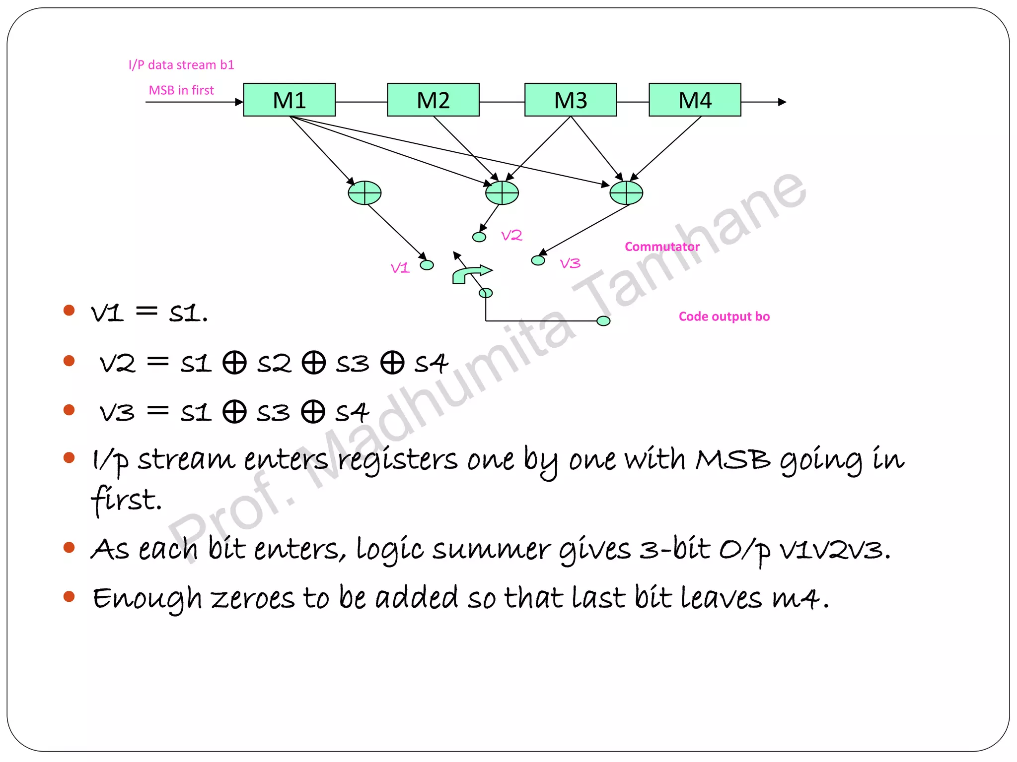
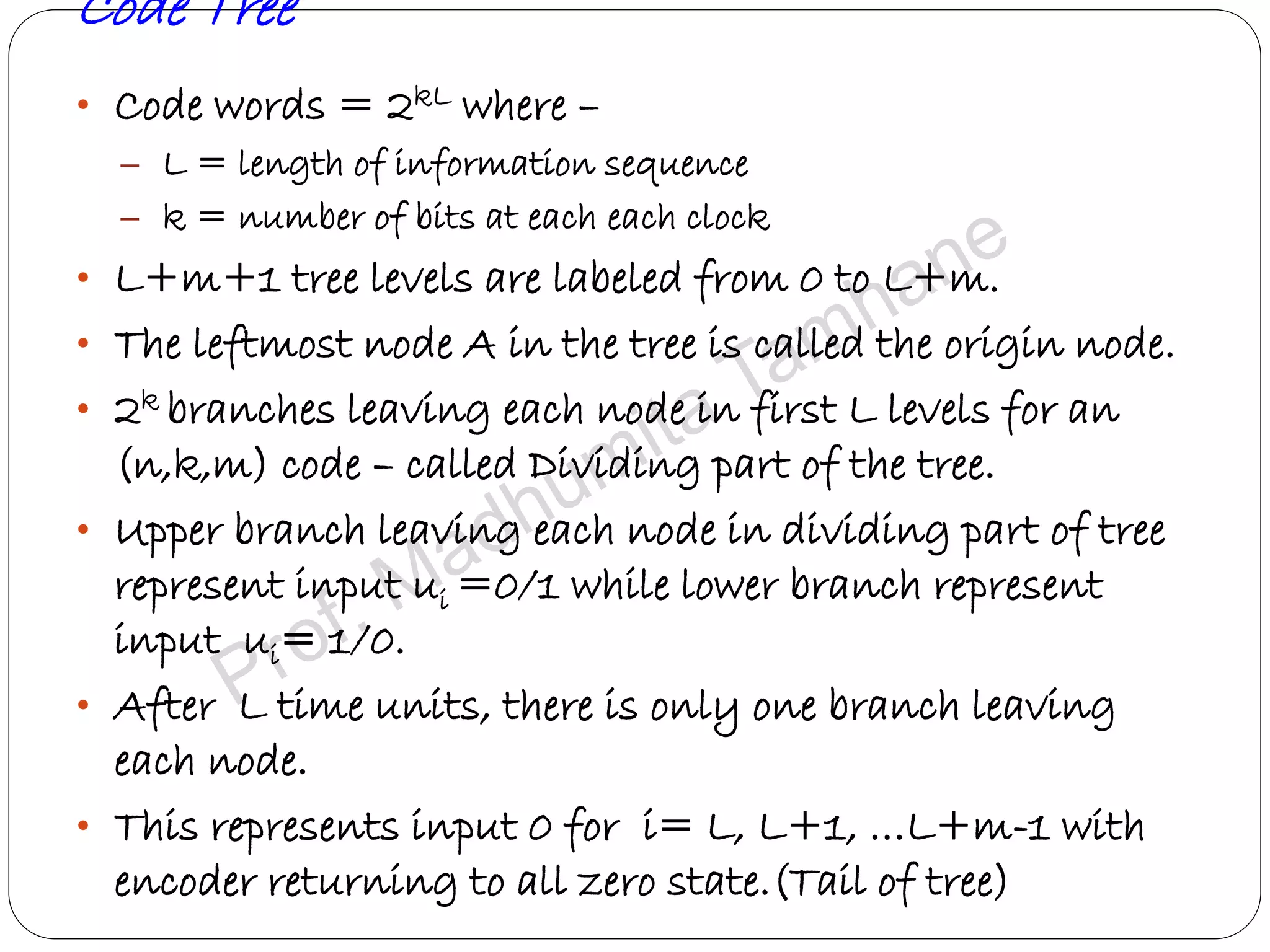
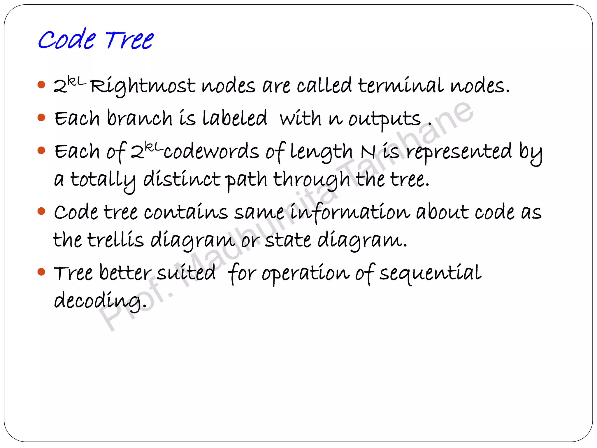
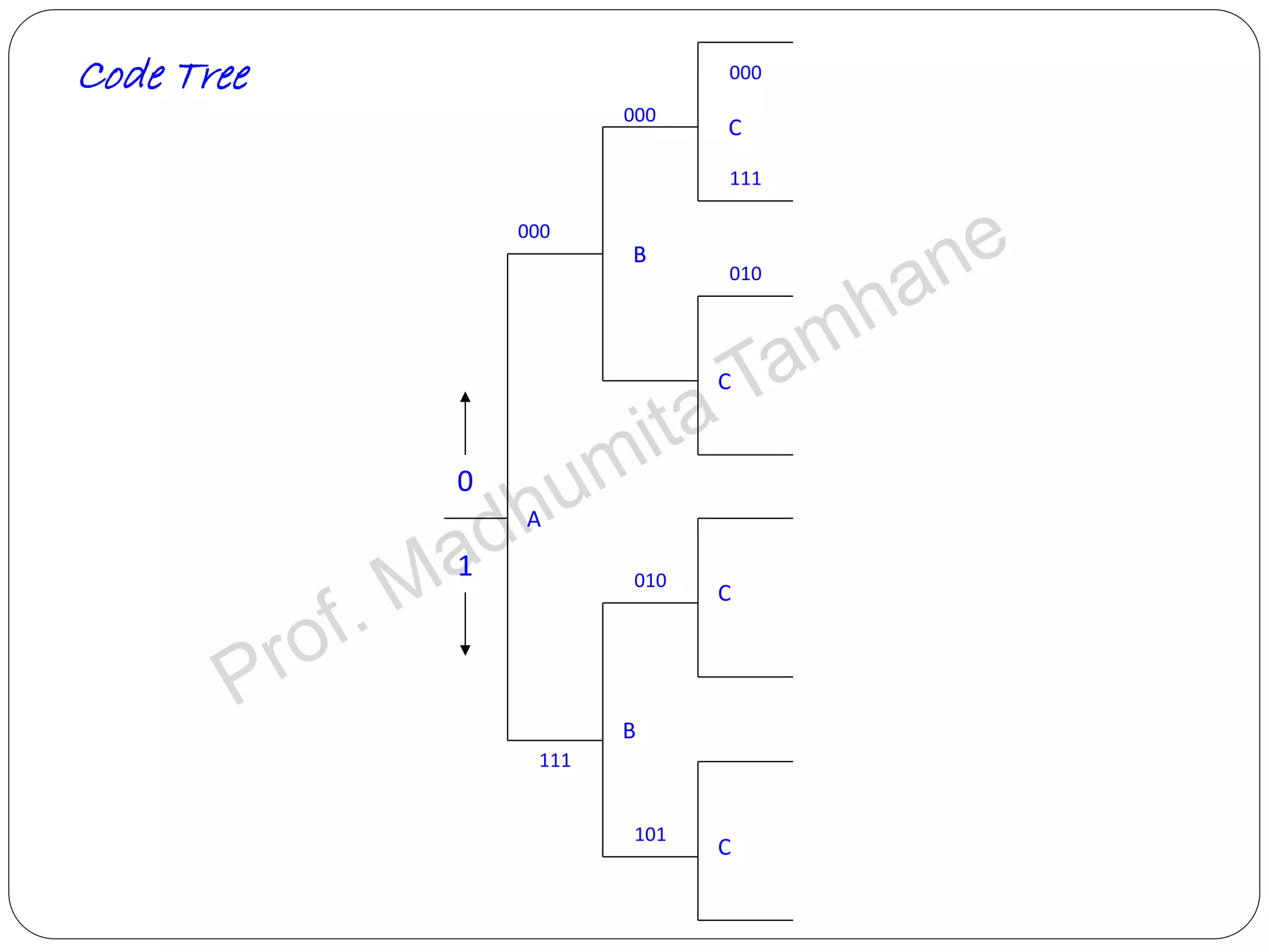
Explains the design and structure of code trees, their functionality, and representation of code words.
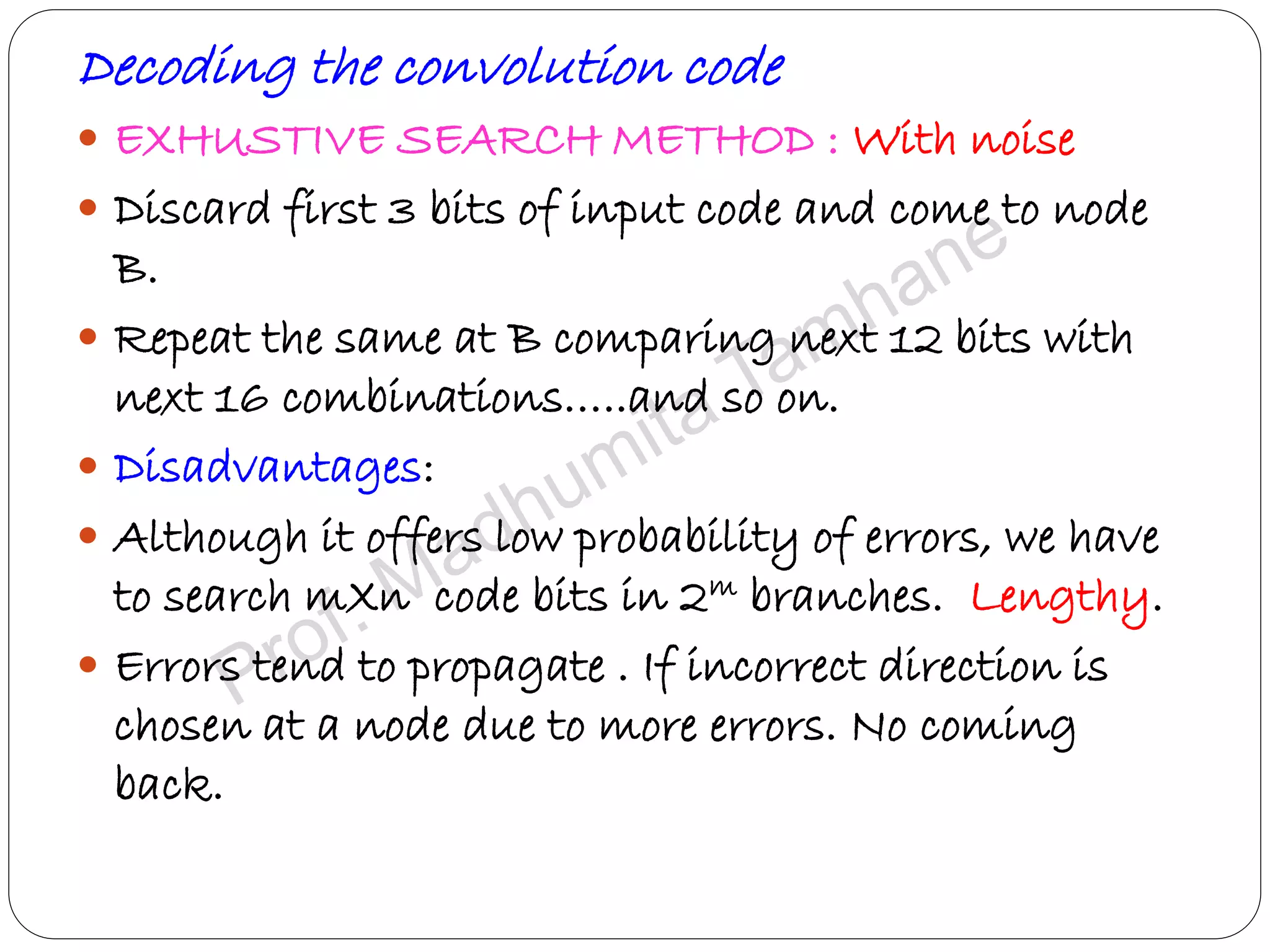
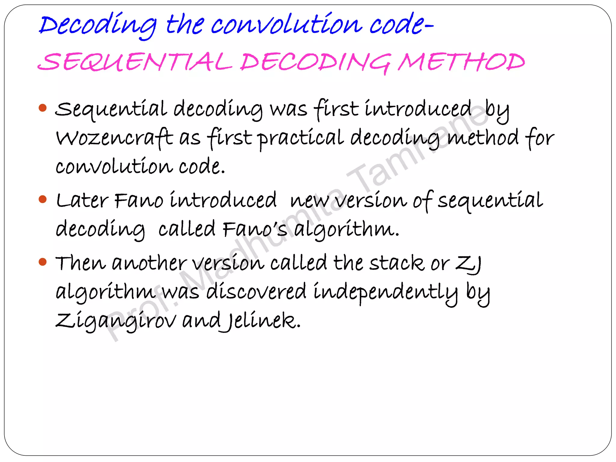
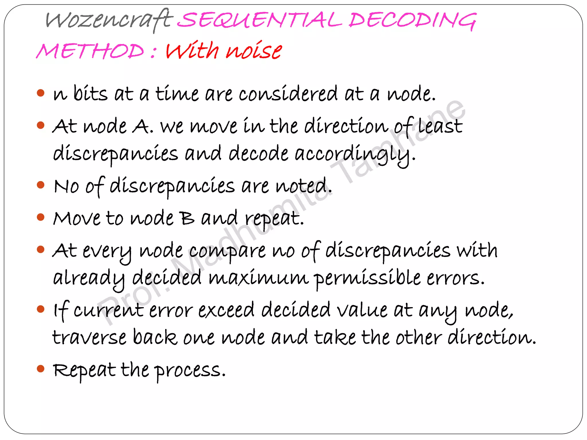
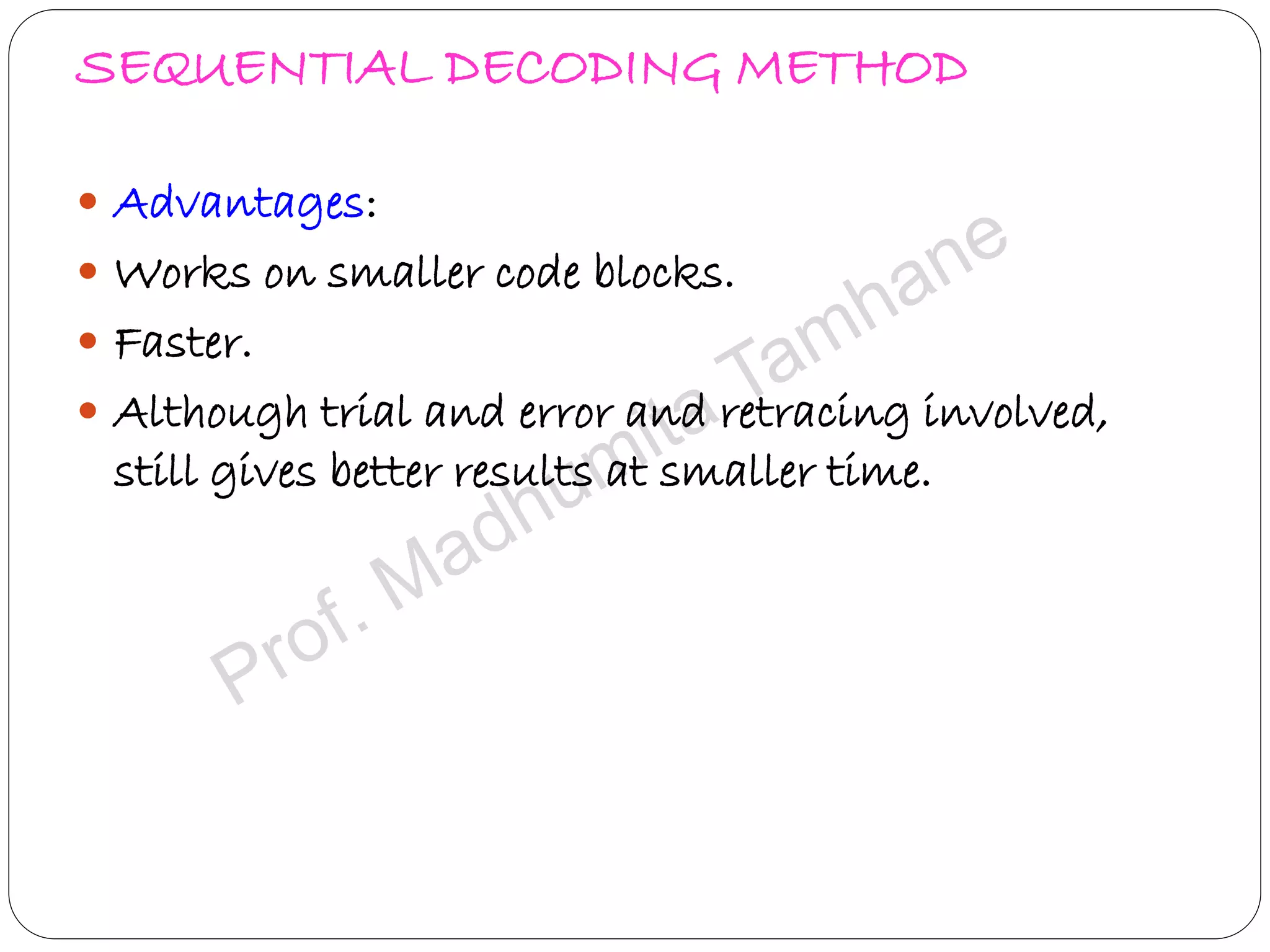
Compares exhaustive search and sequential decoding methods for convolution codes, highlighting advantages.
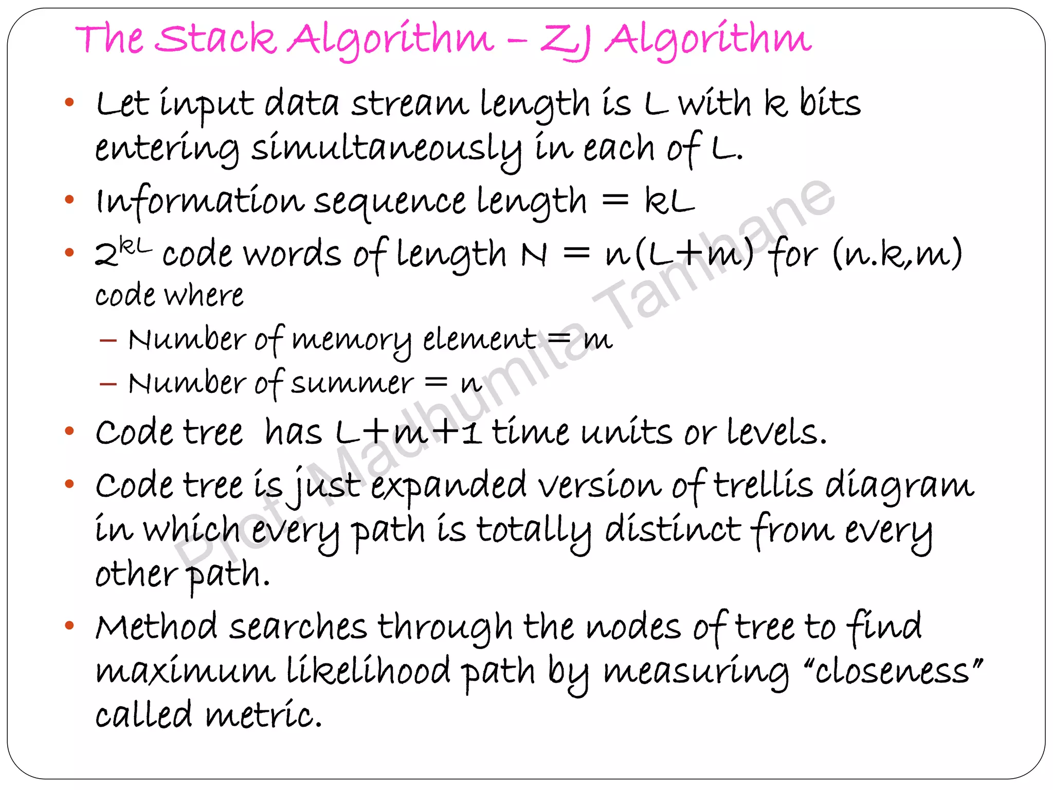
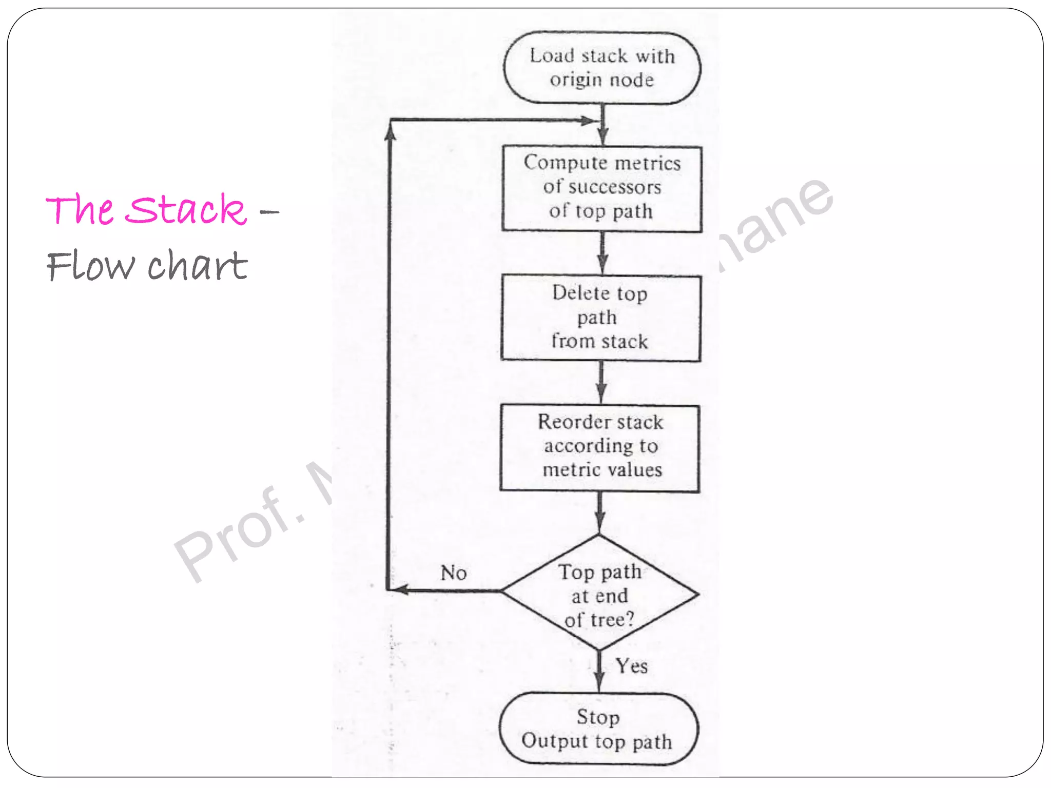
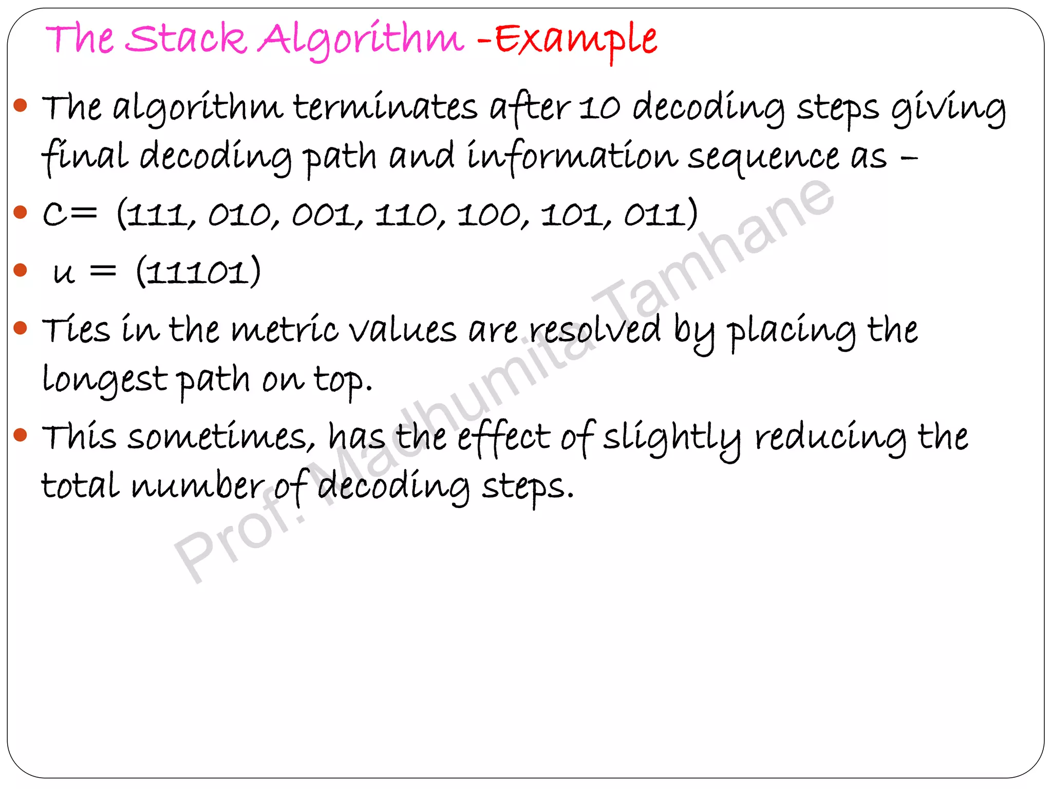
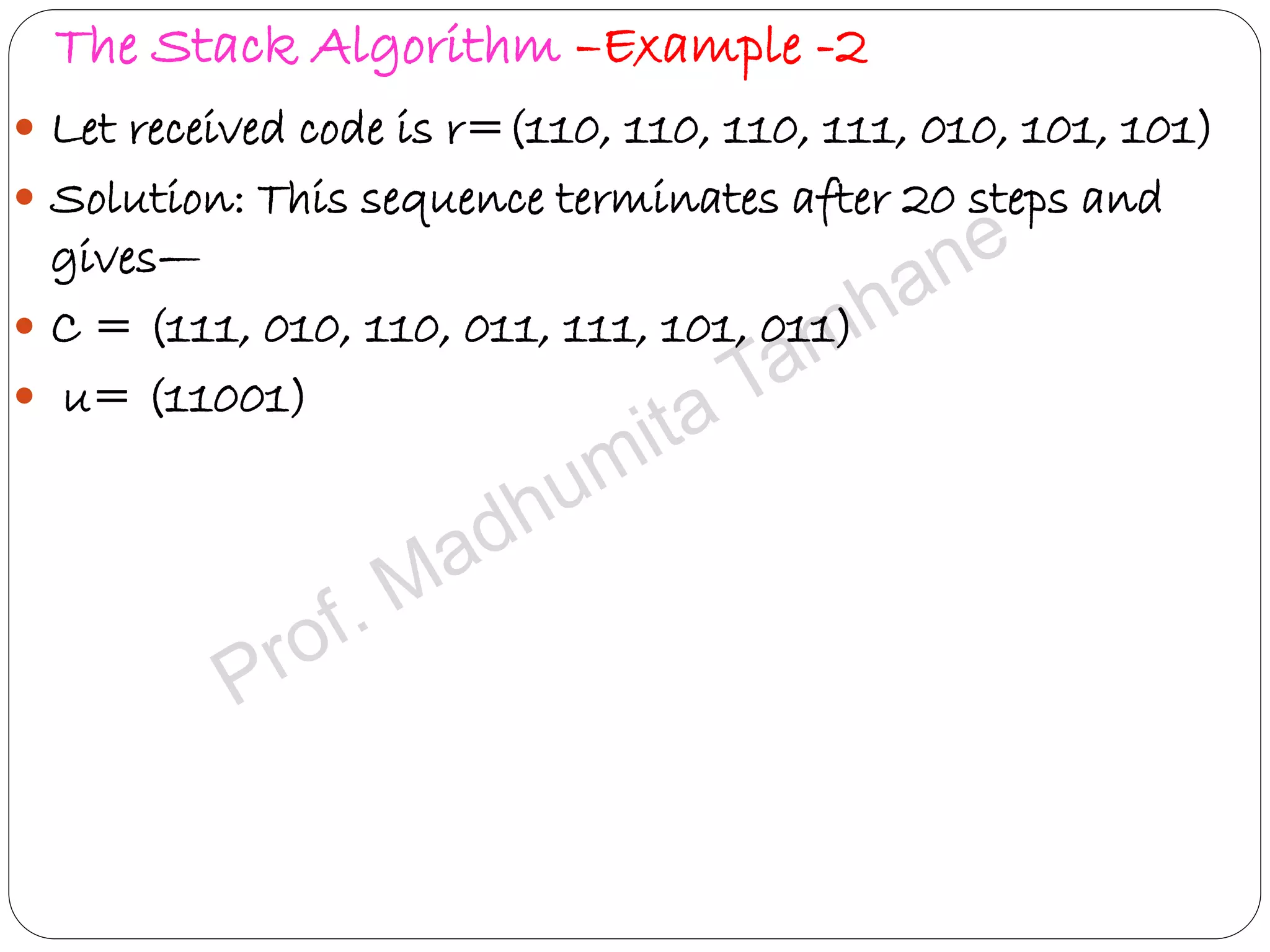
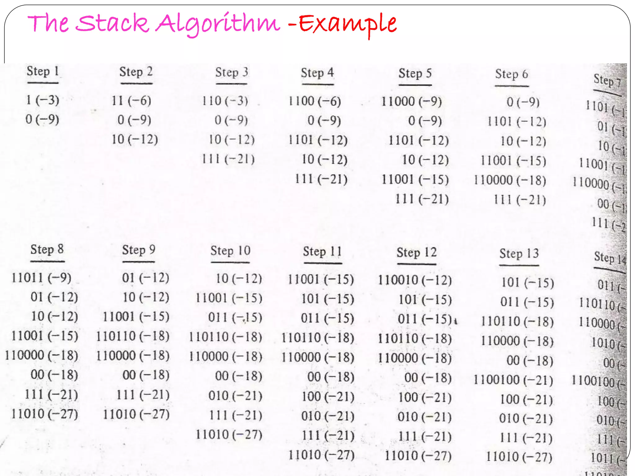
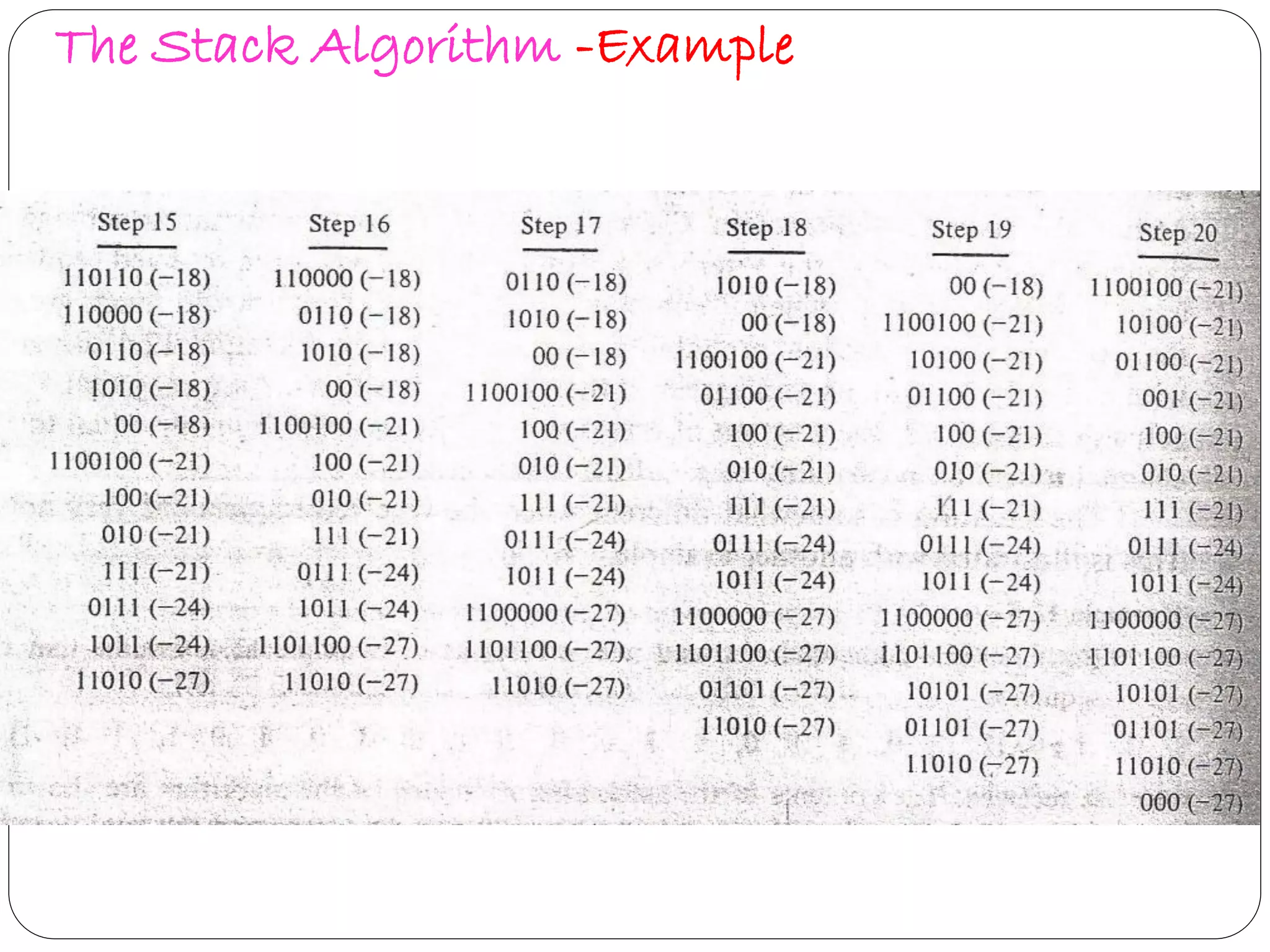
Describes Stack Algorithm methodology, advantages, limitations, and flow workflows in decoding.
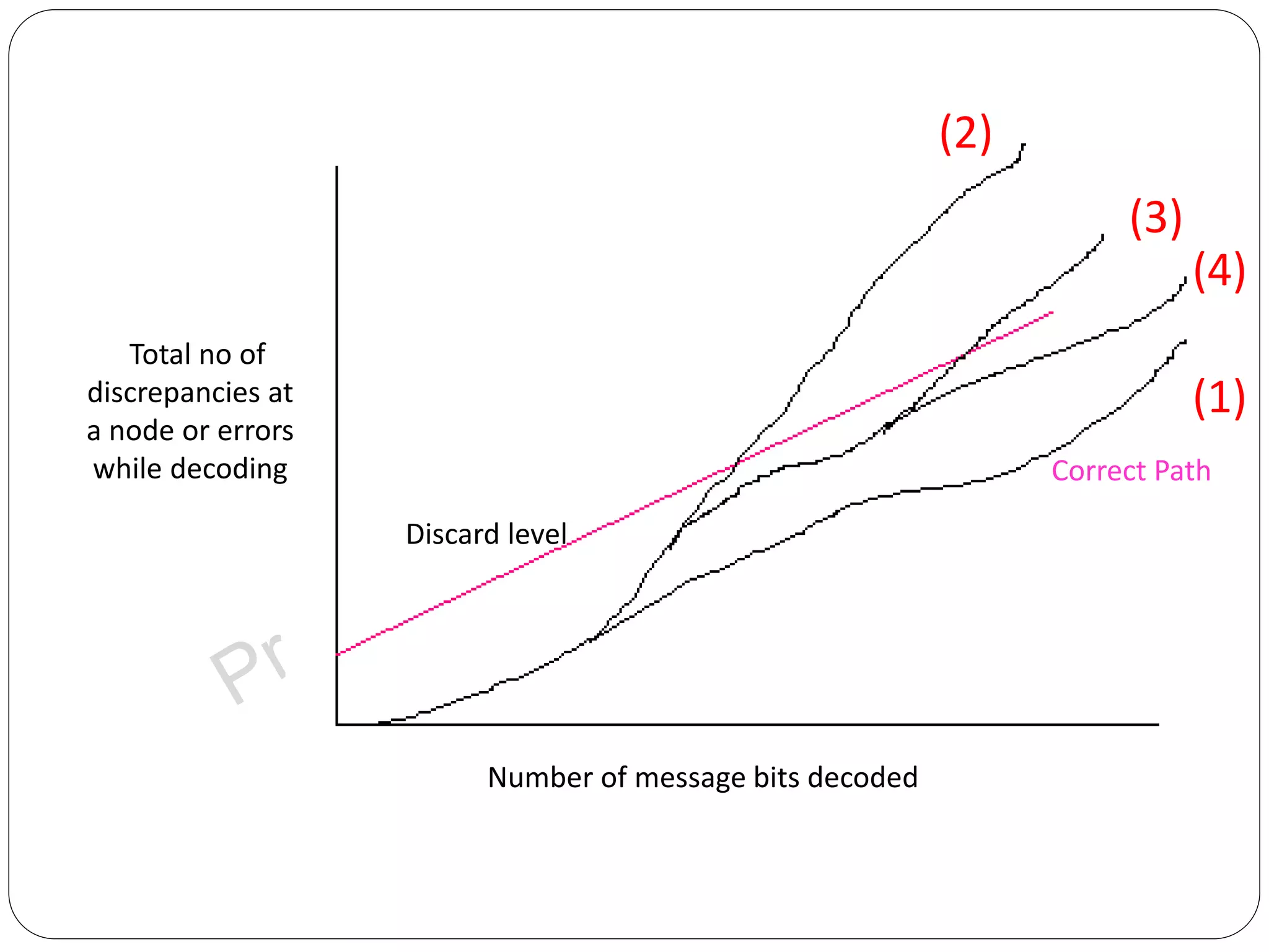
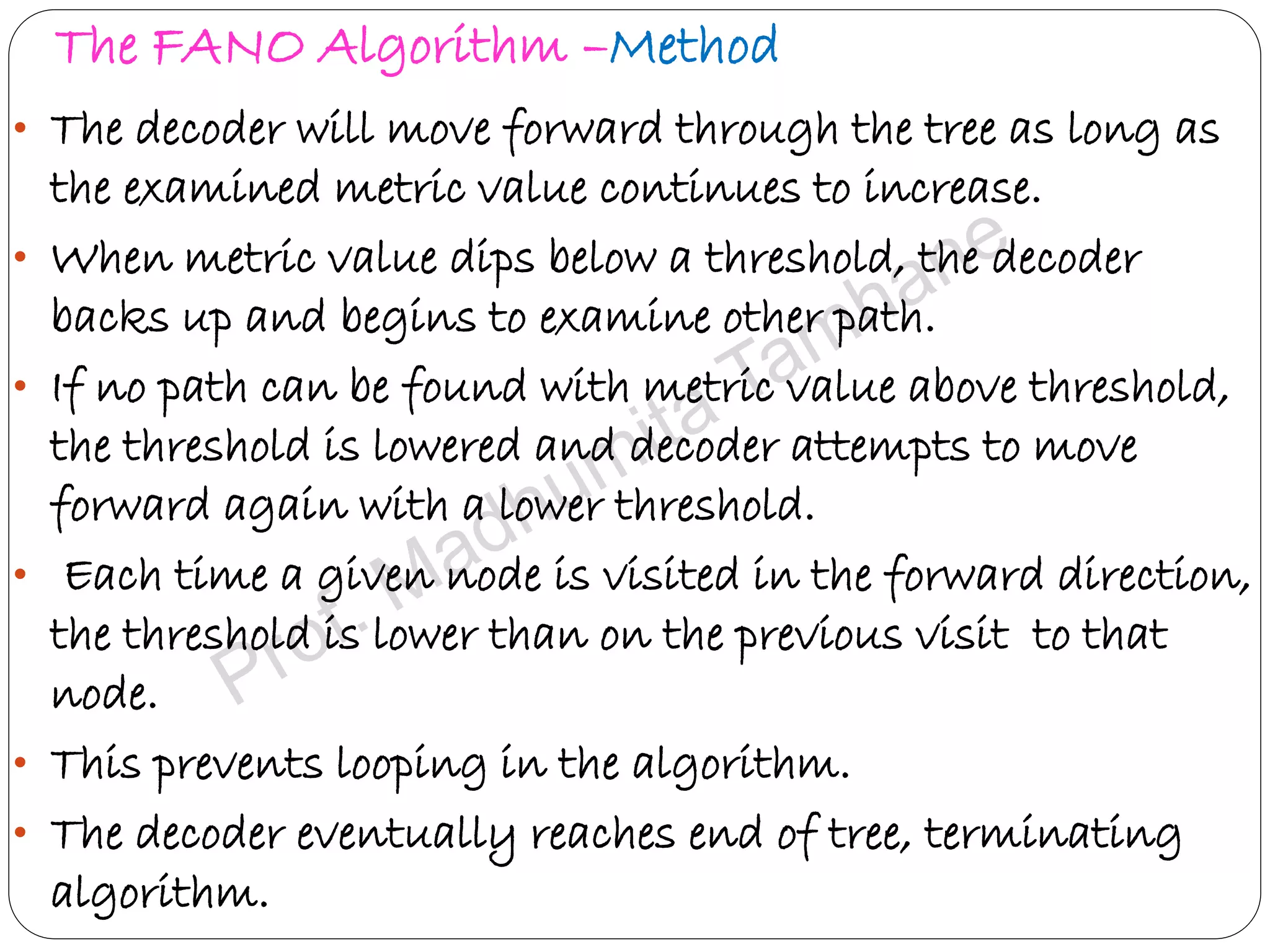
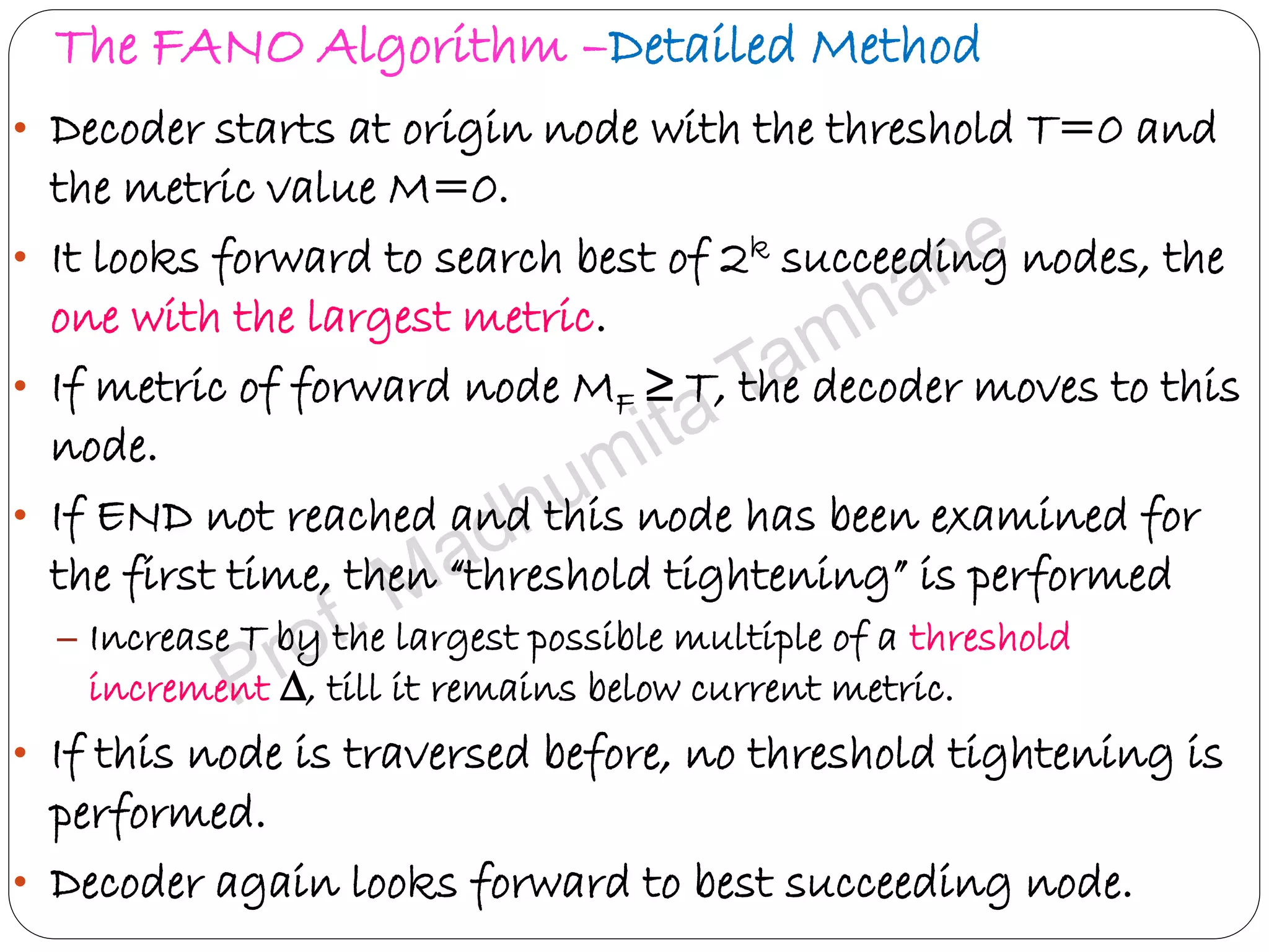
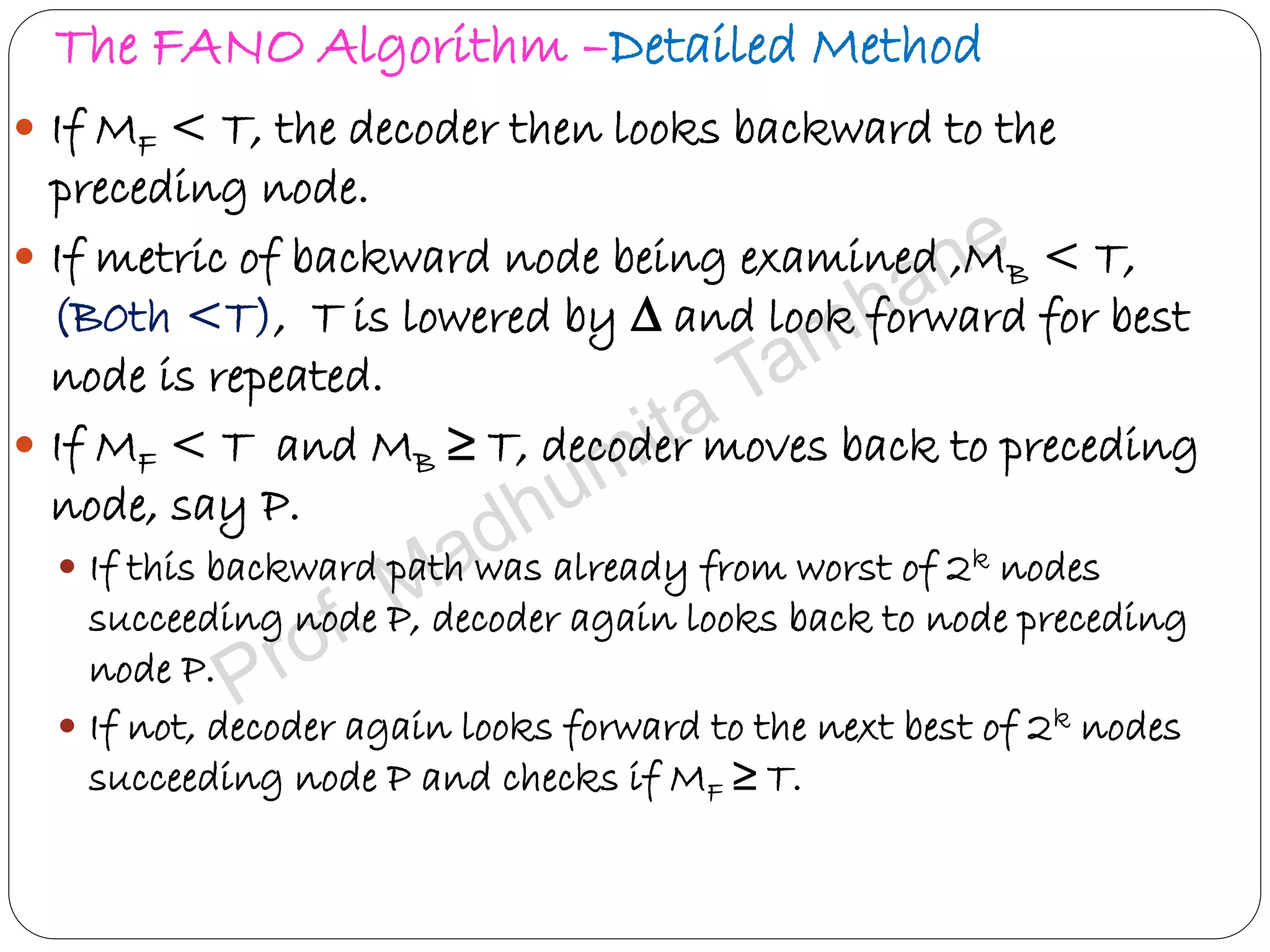
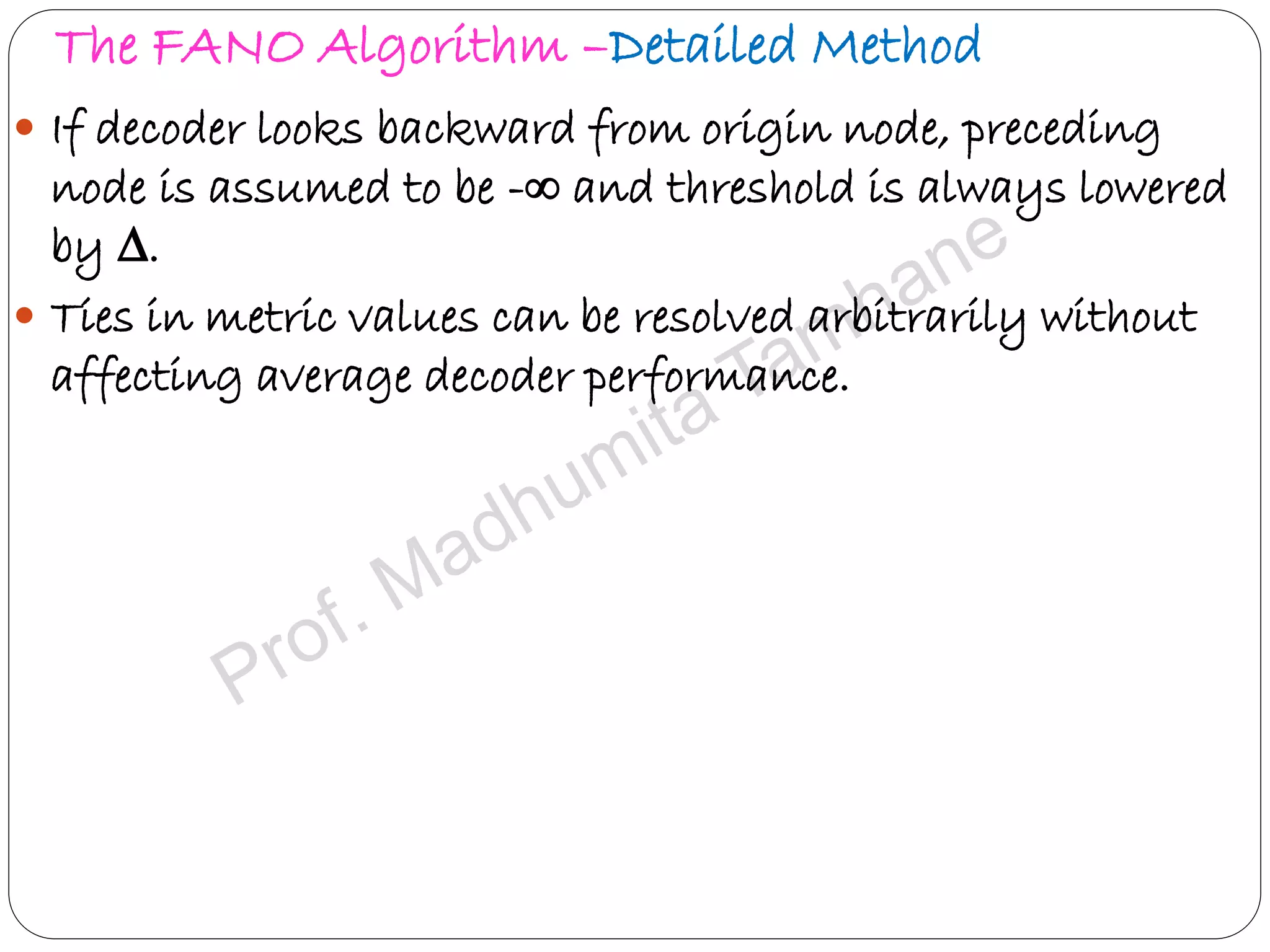
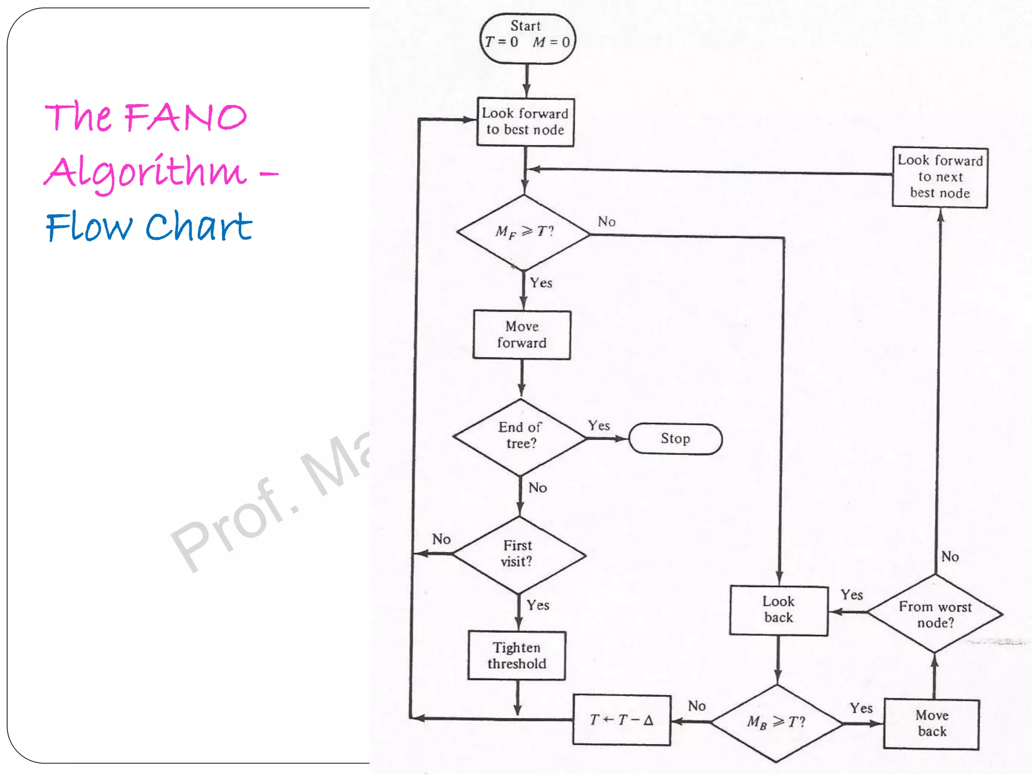
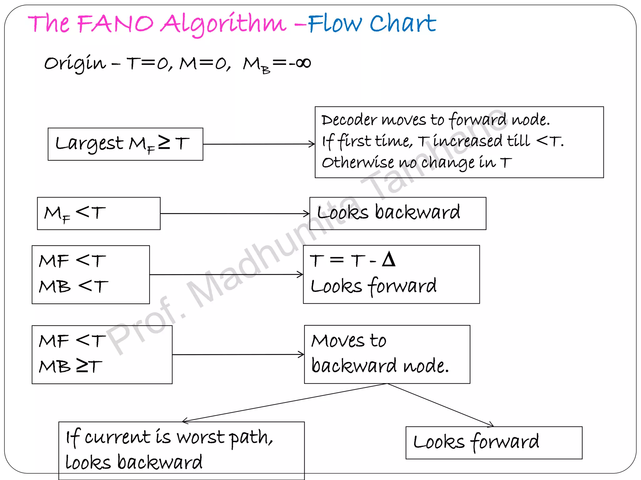
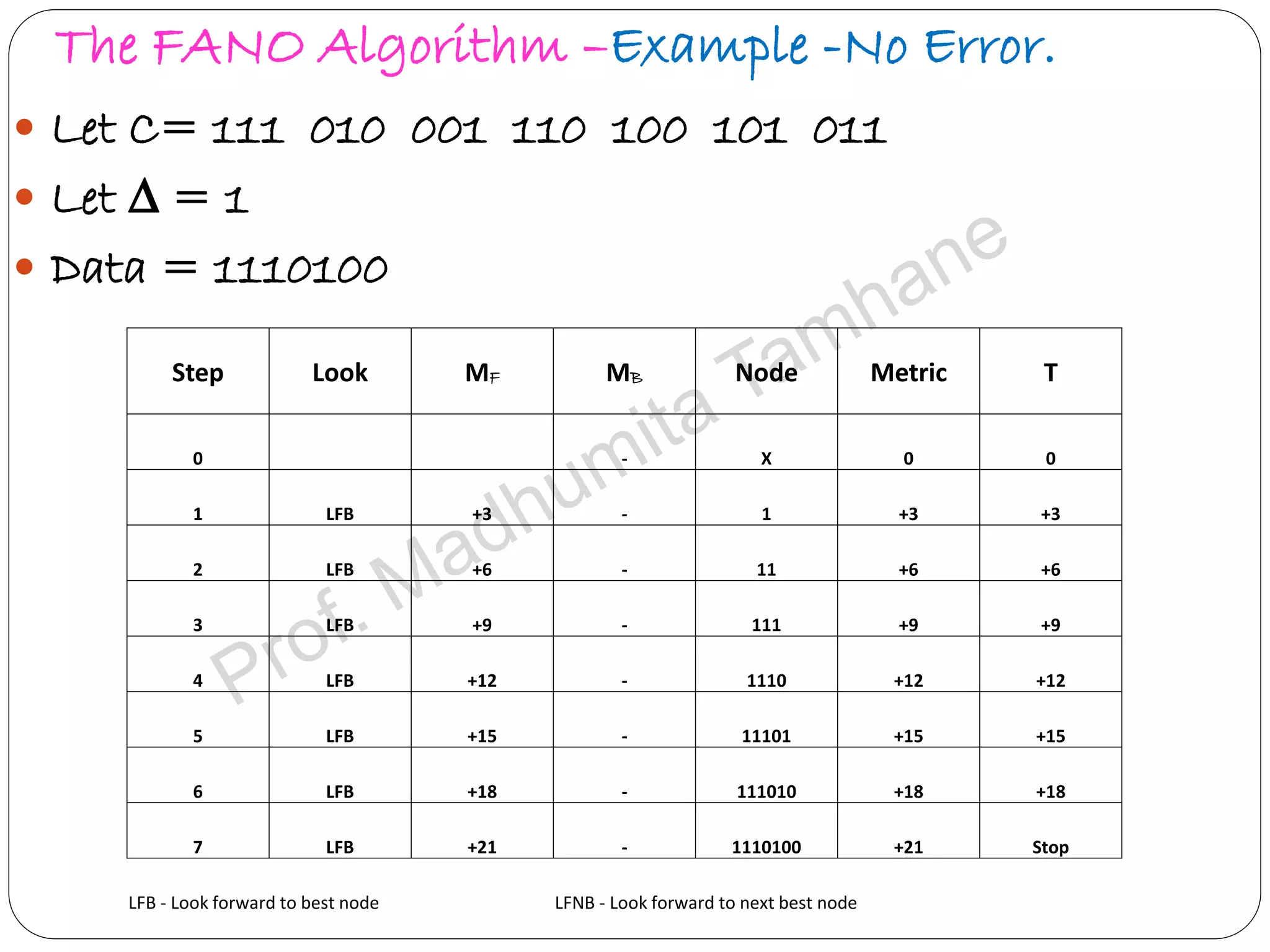
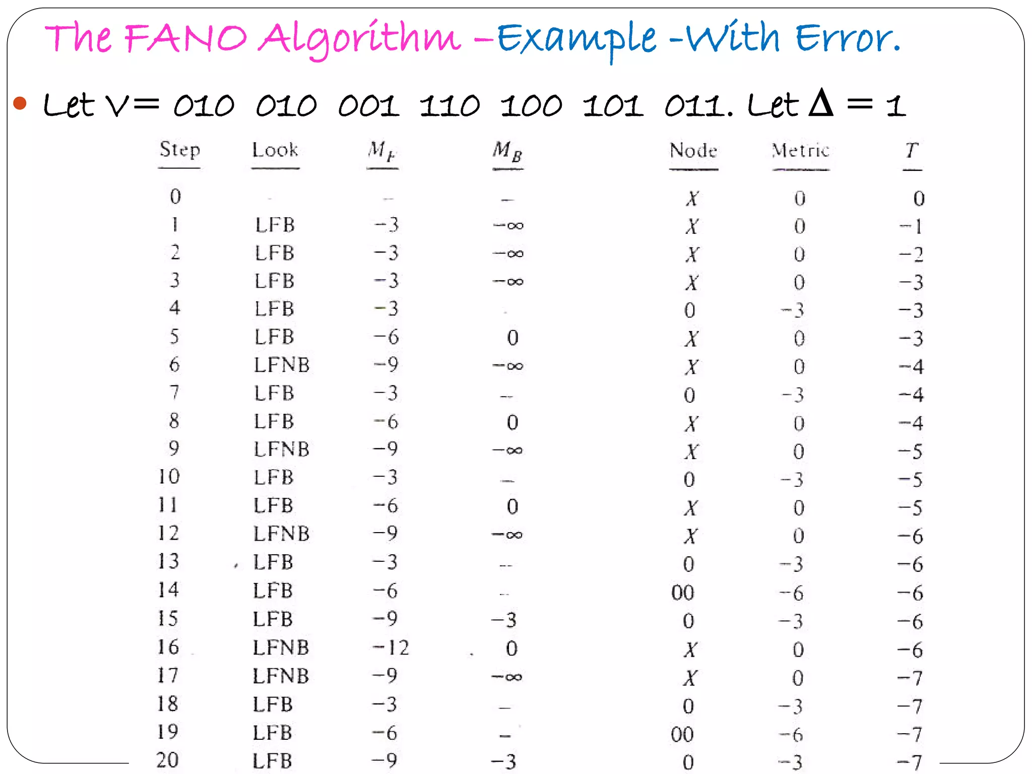
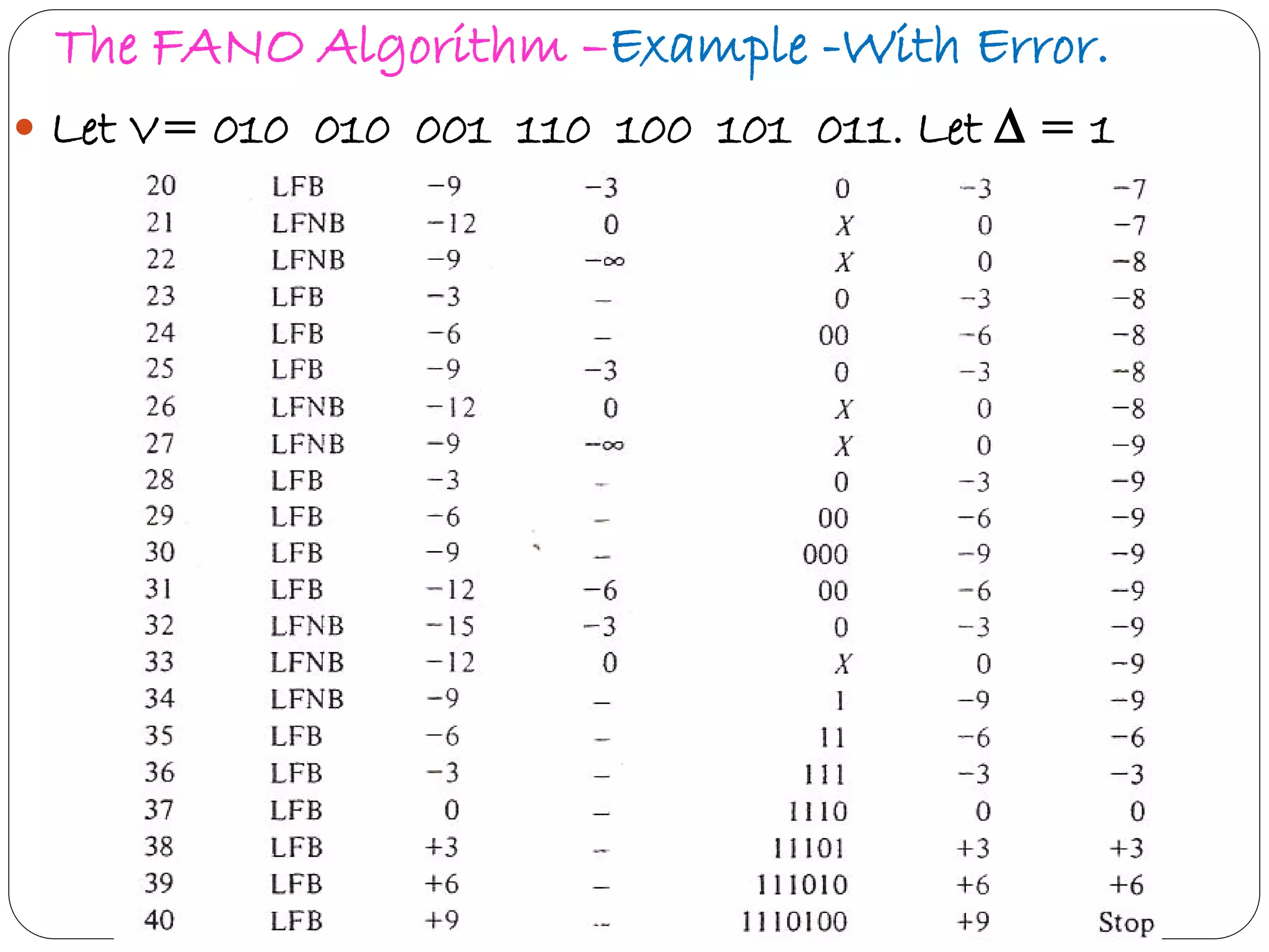
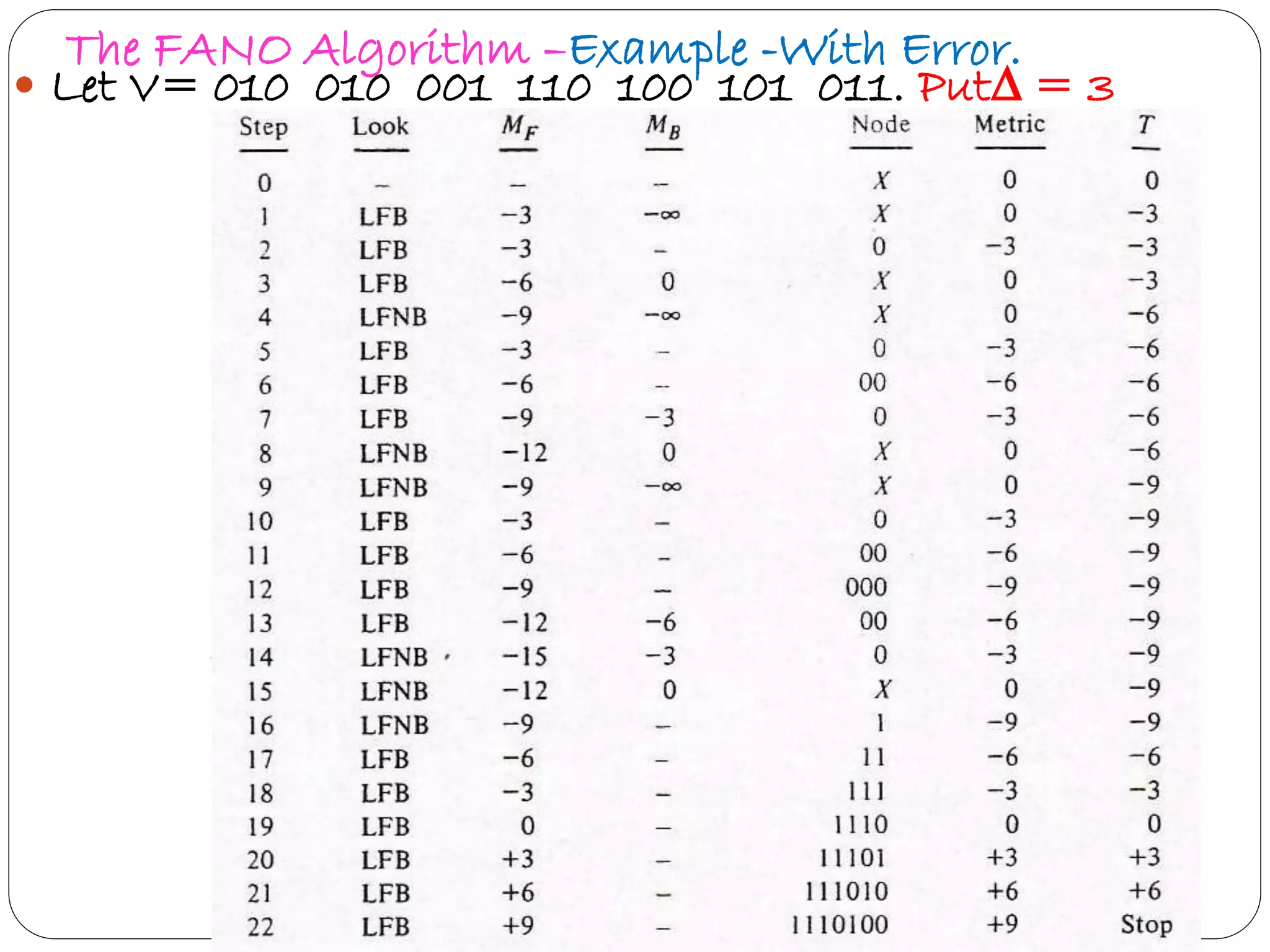
Explains Fano algorithm details, its method of trajectory through tree nodes, and limitations.