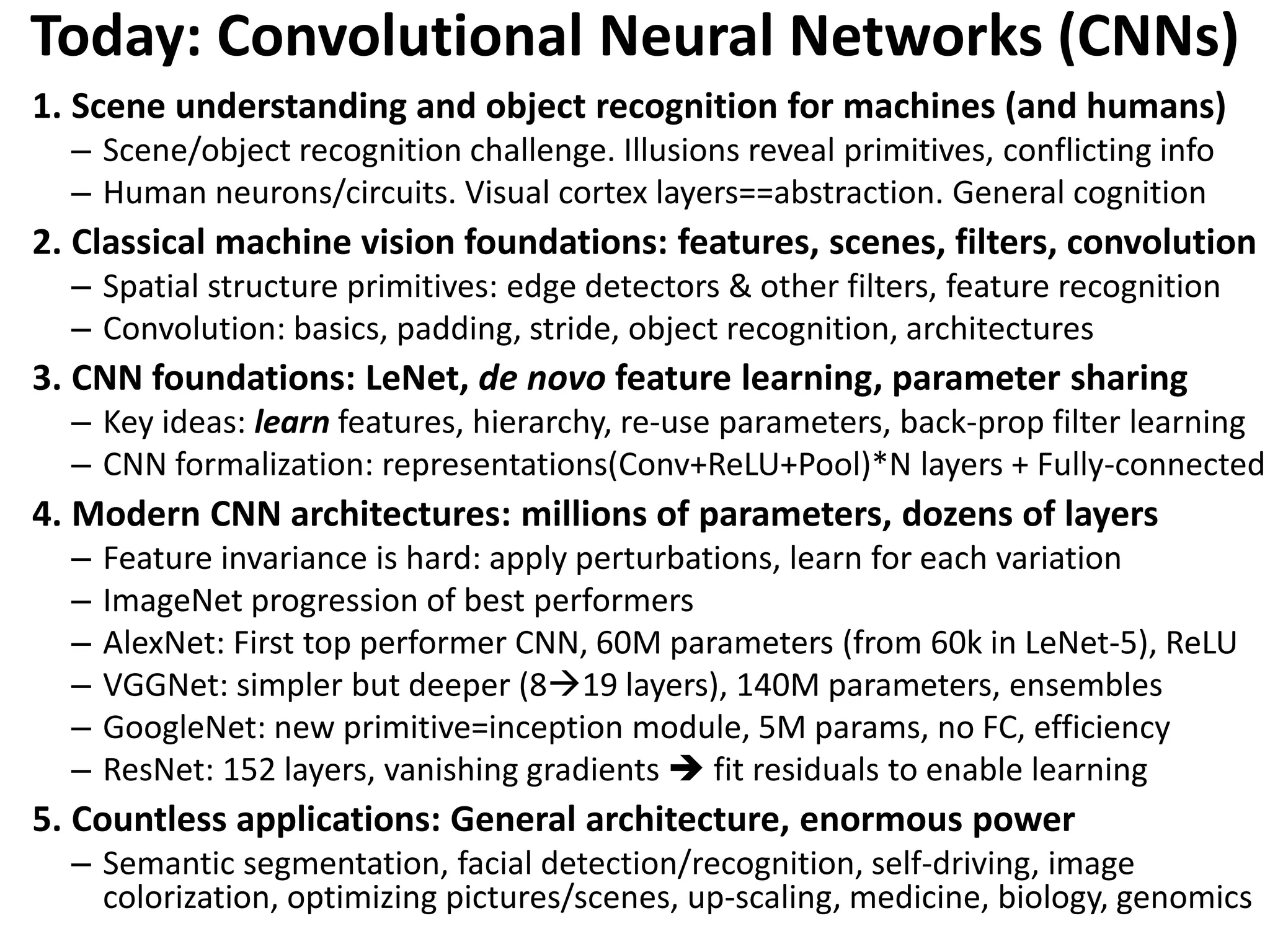
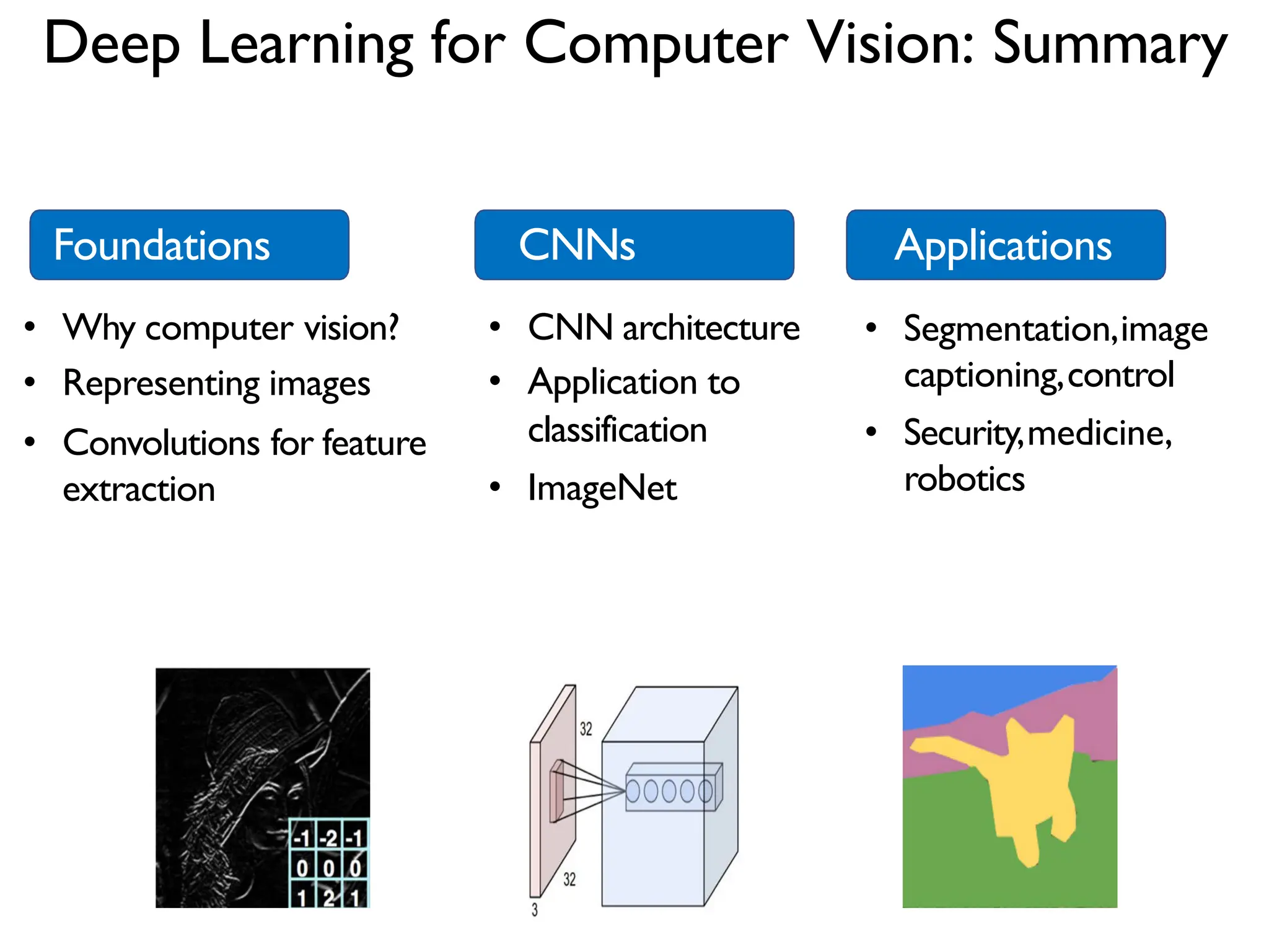
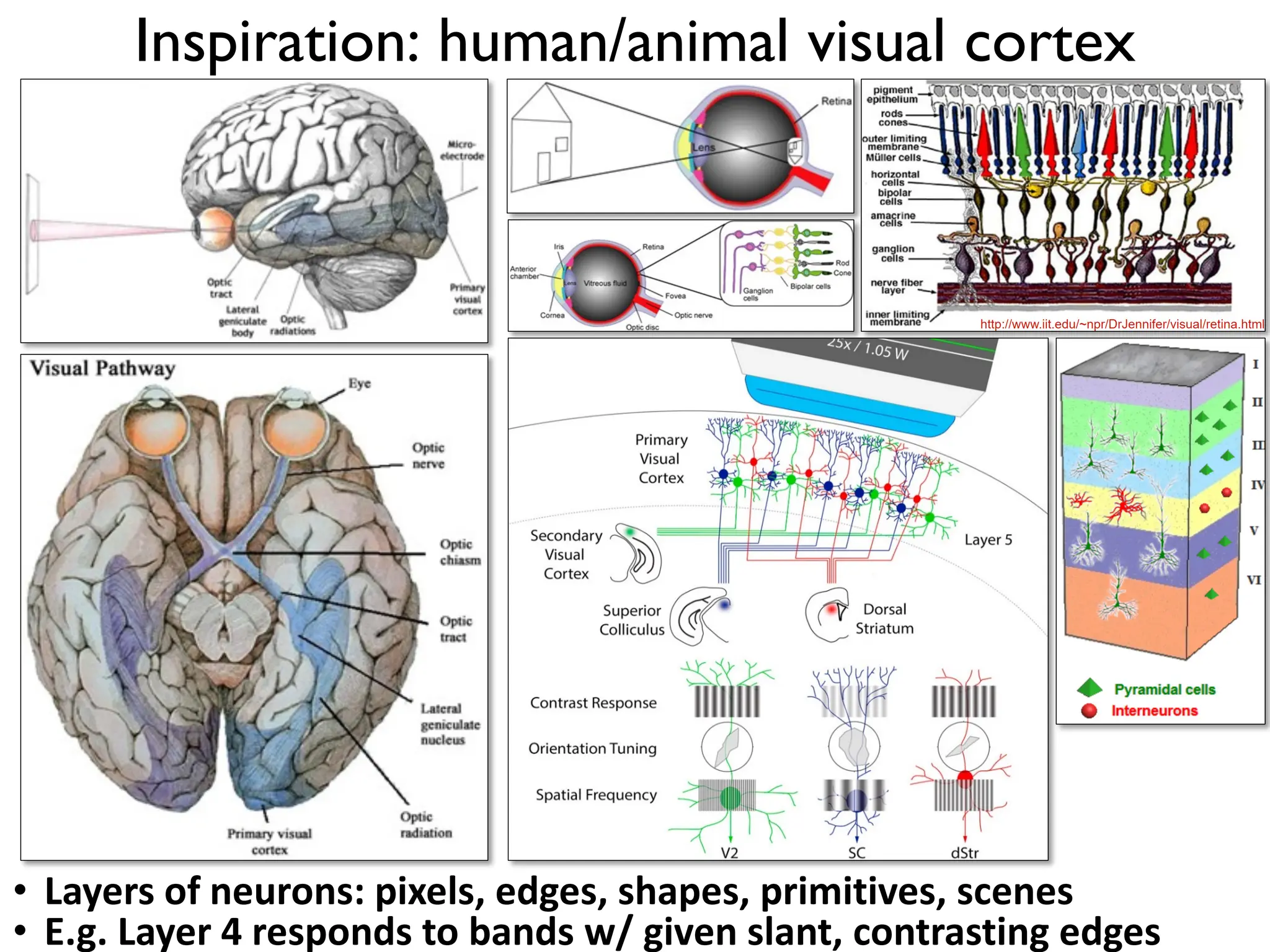
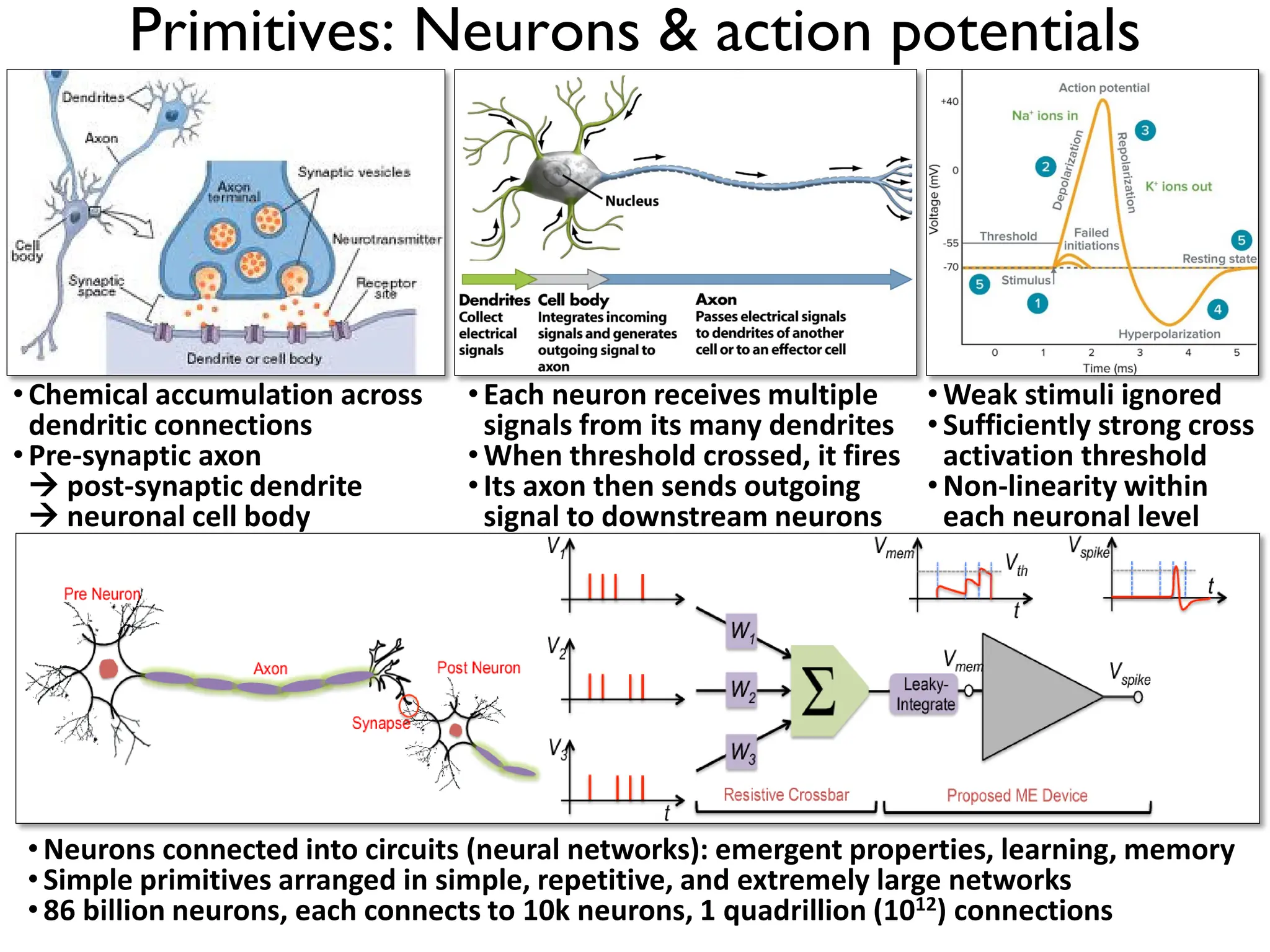
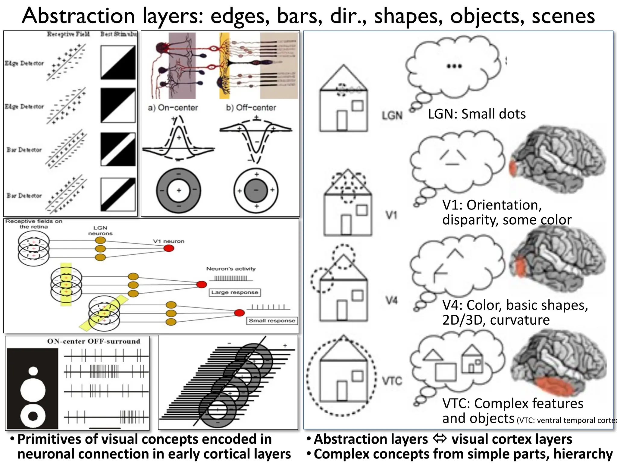
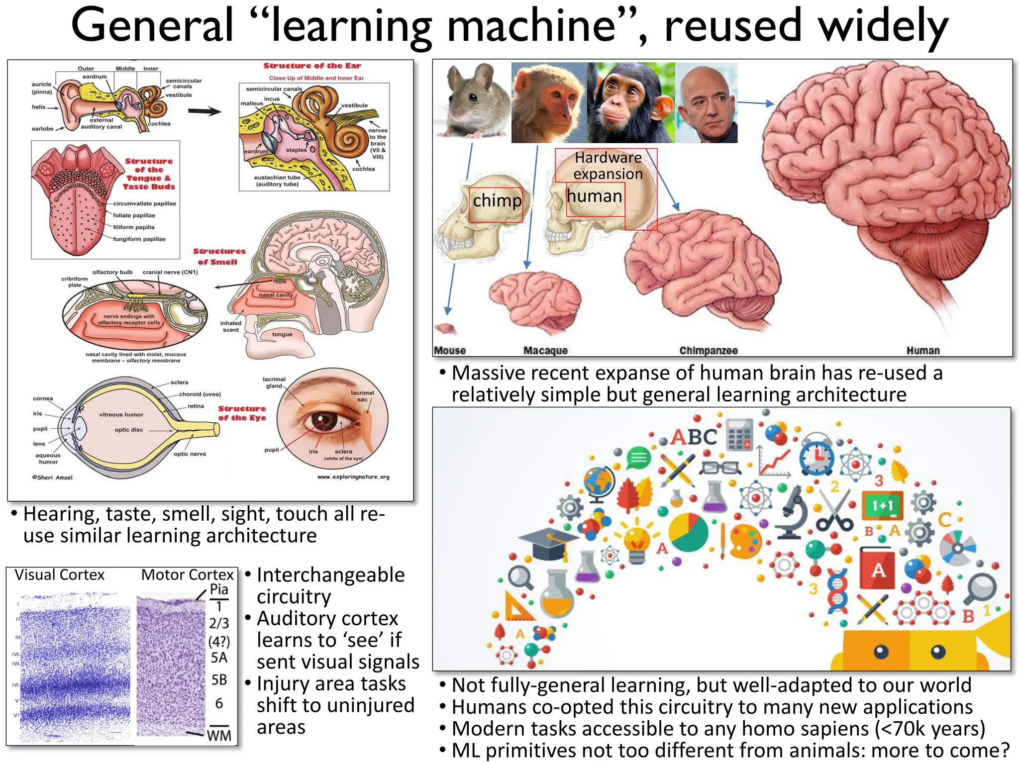
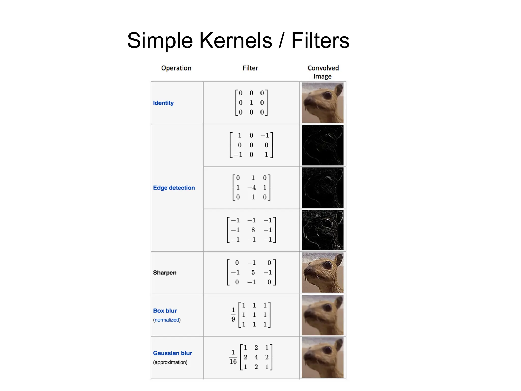
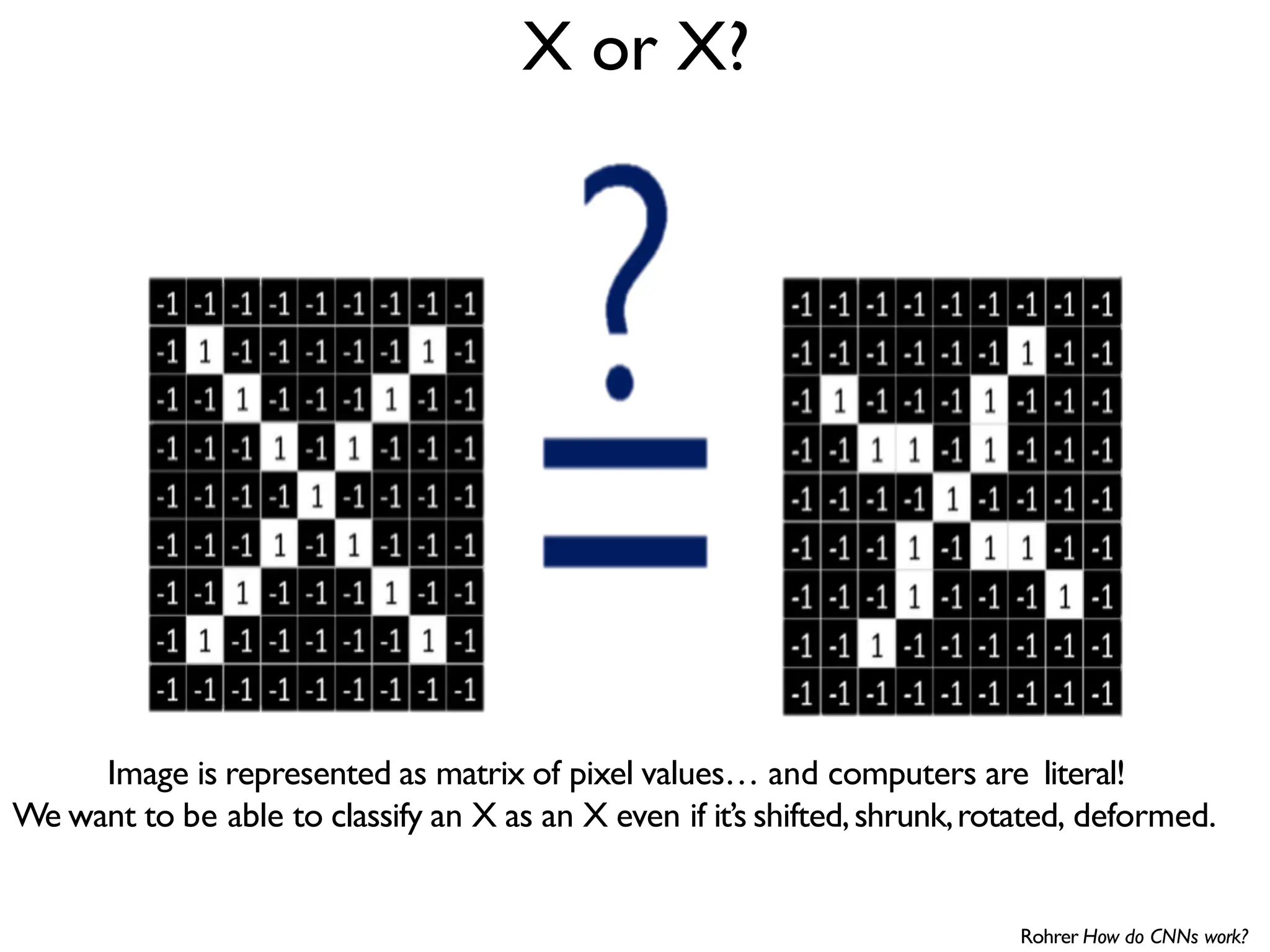
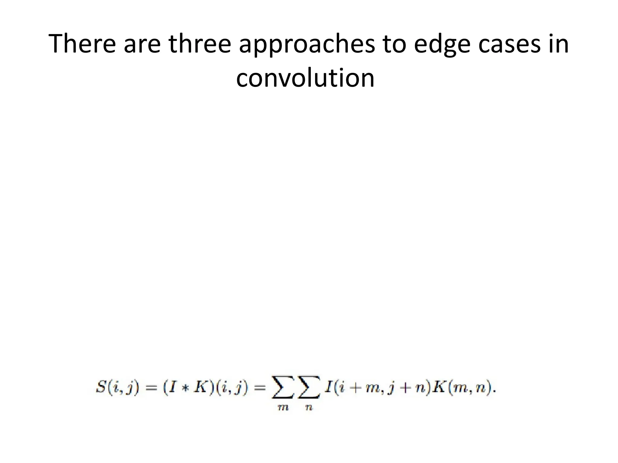
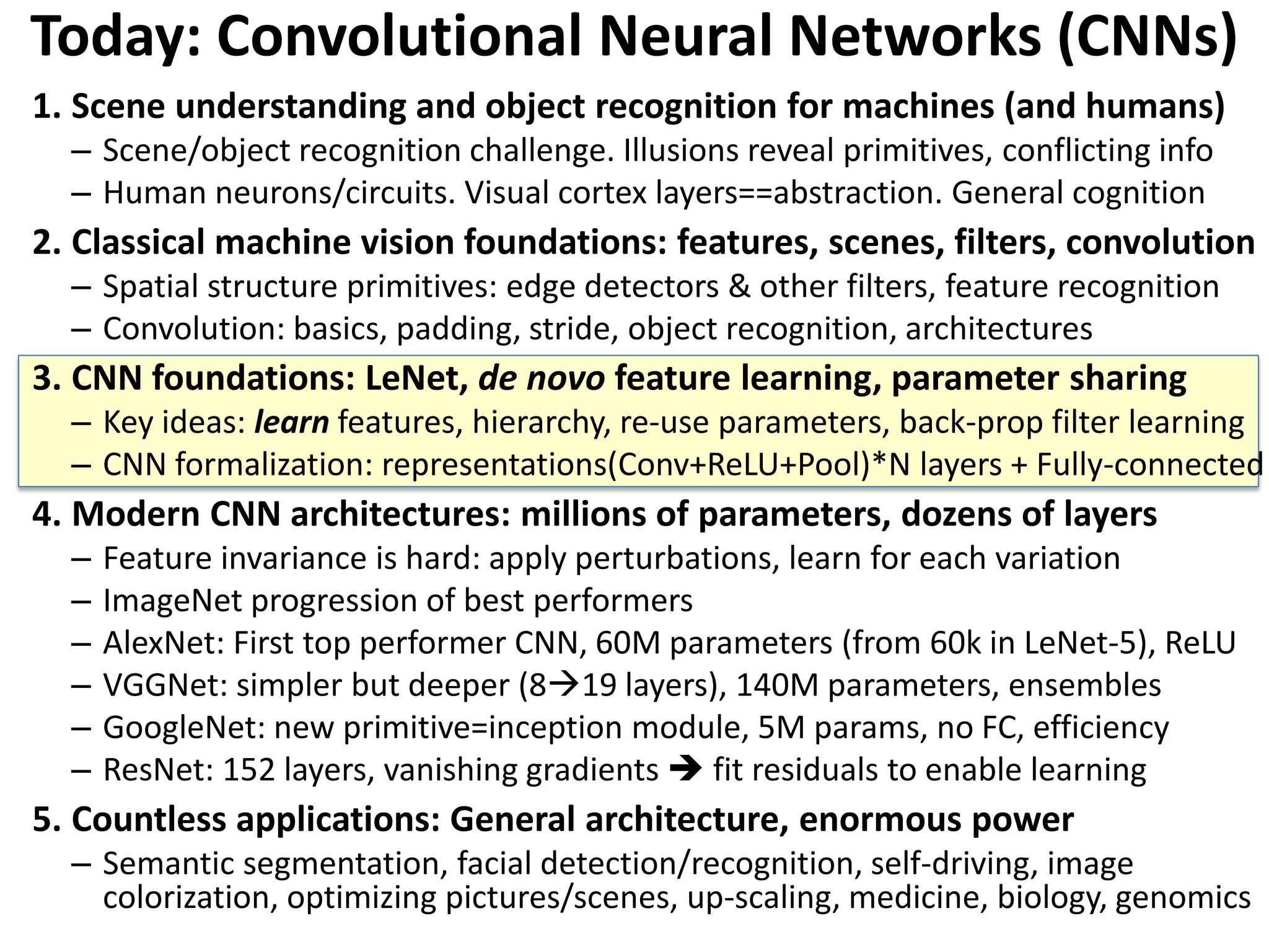
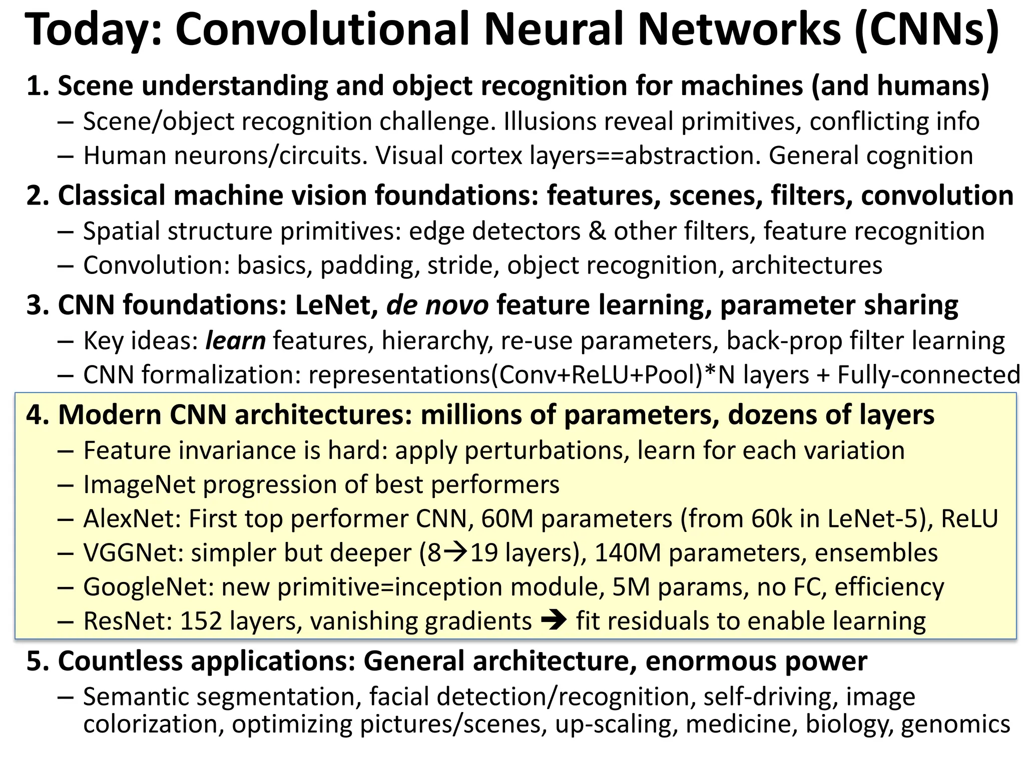
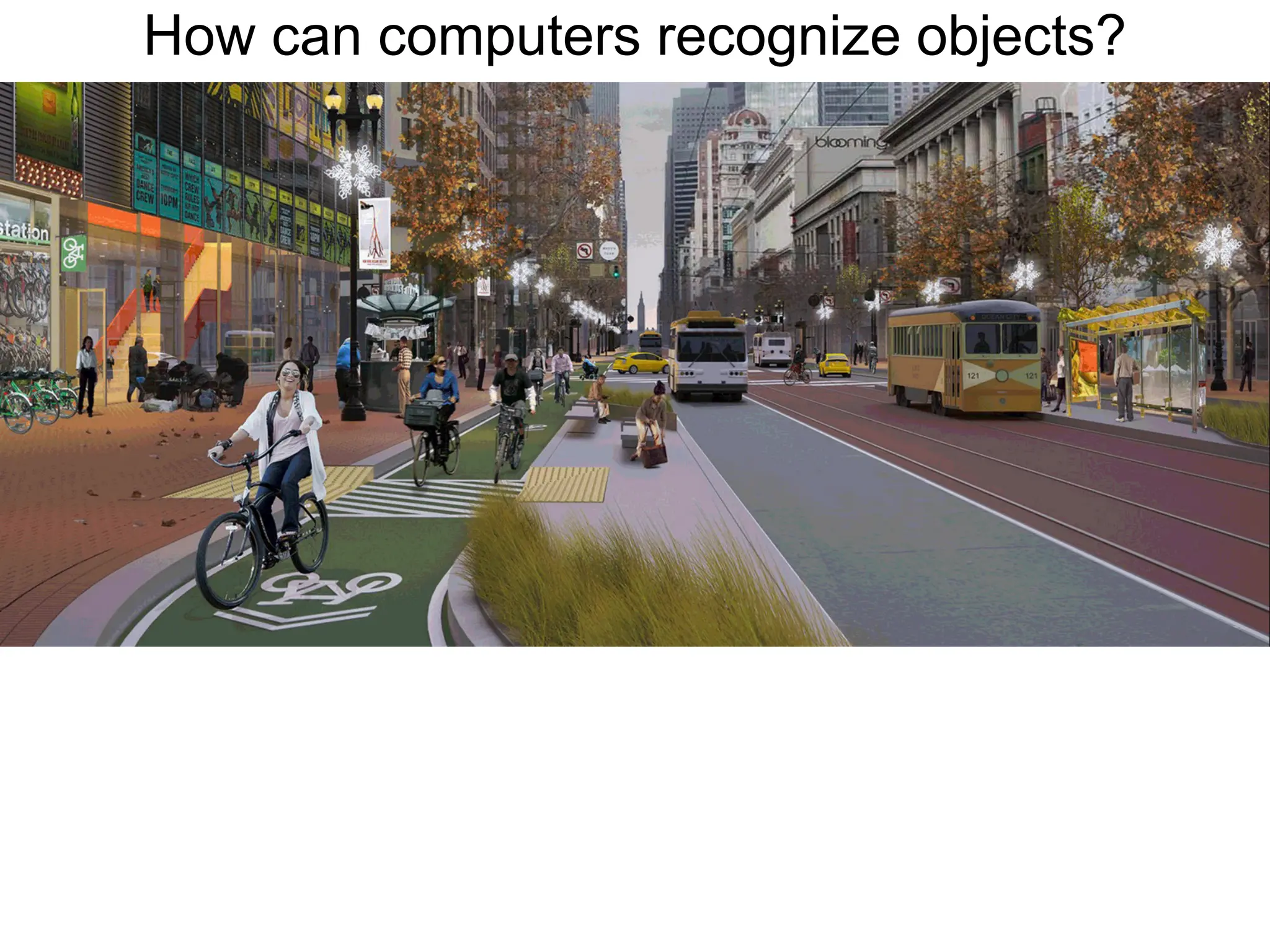
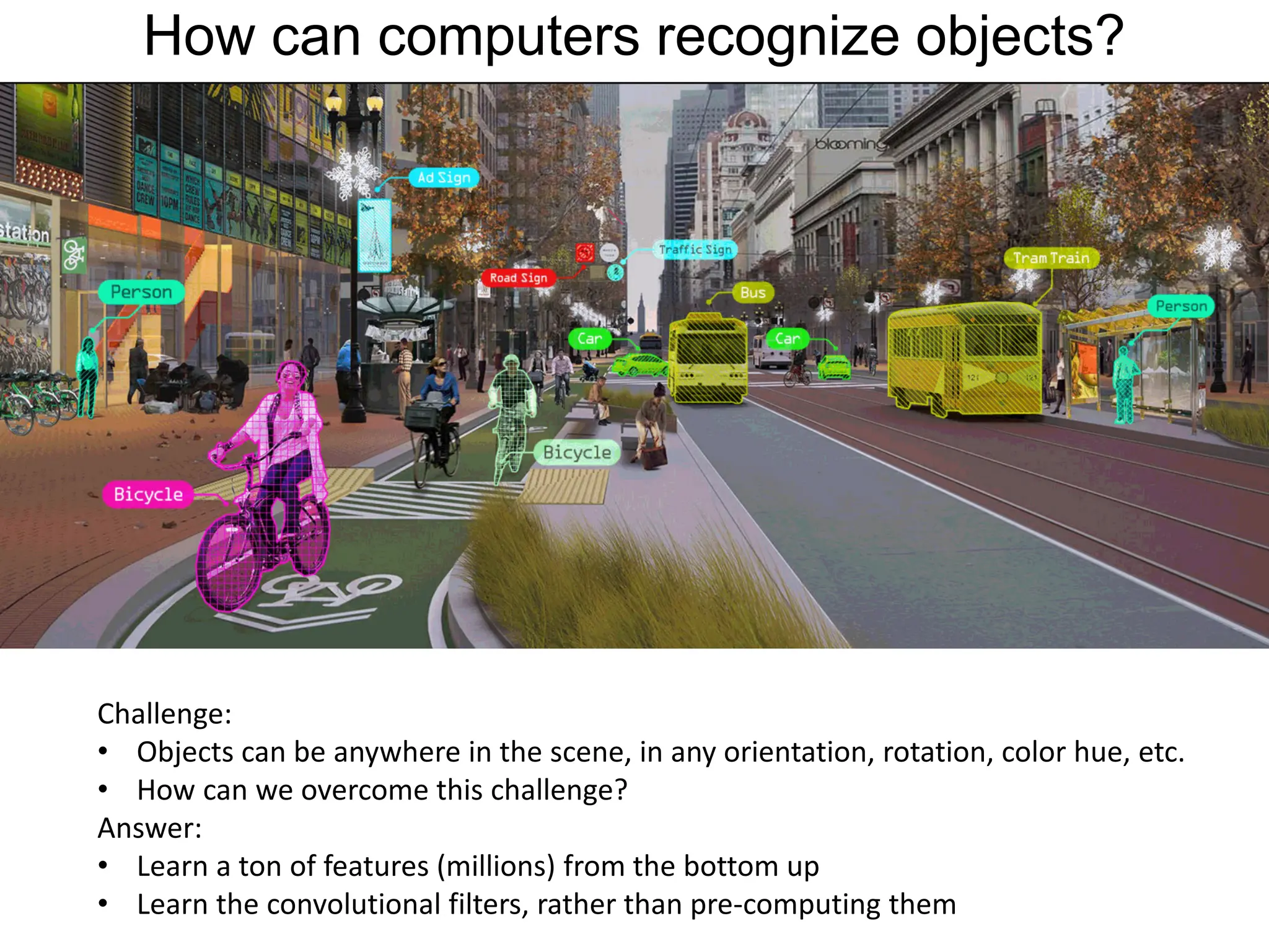
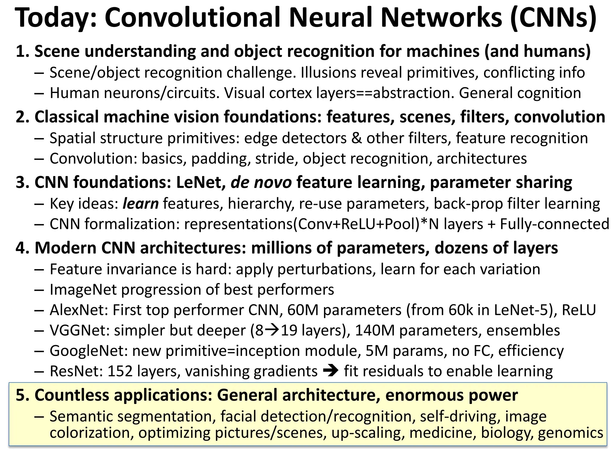
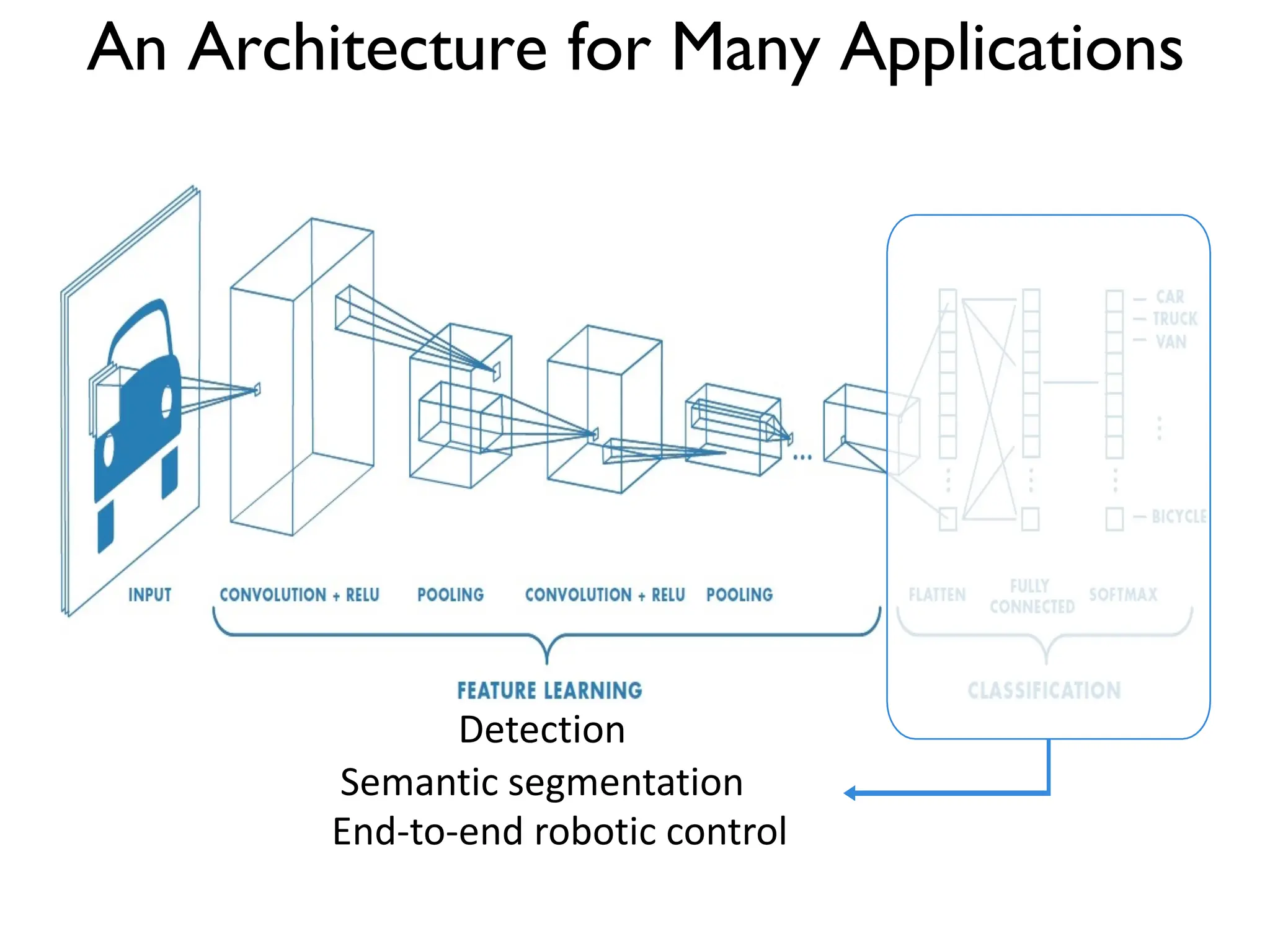
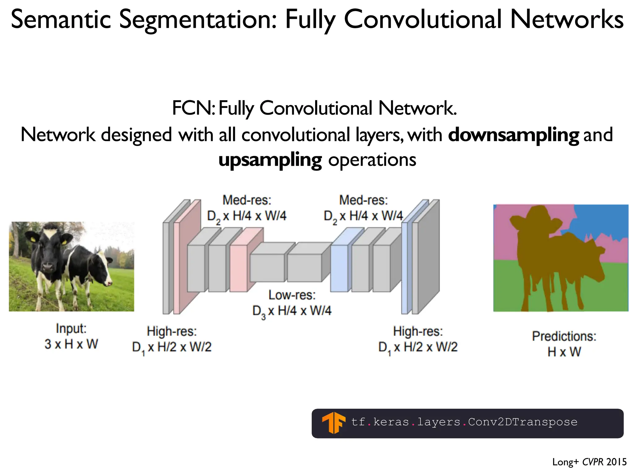
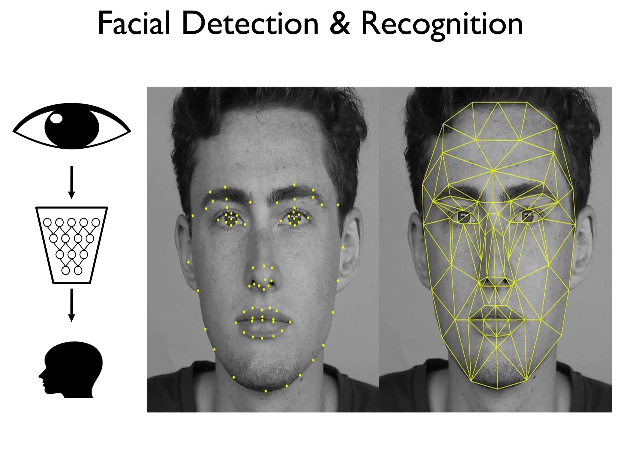
1. The document discusses Convolutional Neural Networks (CNNs) for object recognition and scene understanding. It covers the biological inspiration from the human visual cortex, classical computer vision techniques, and the foundations of CNNs including LeNet and learning visual features. 2. CNNs apply successive layers of convolutions, nonlinear activations, and pooling to learn hierarchical representations of images. Modern CNN architectures have millions of parameters and dozens of layers to learn increasingly complex features. 3. CNNs have countless applications in areas like image classification, segmentation, detection, generation, and more due to their general architecture for learning spatial hierarchies of features from data.
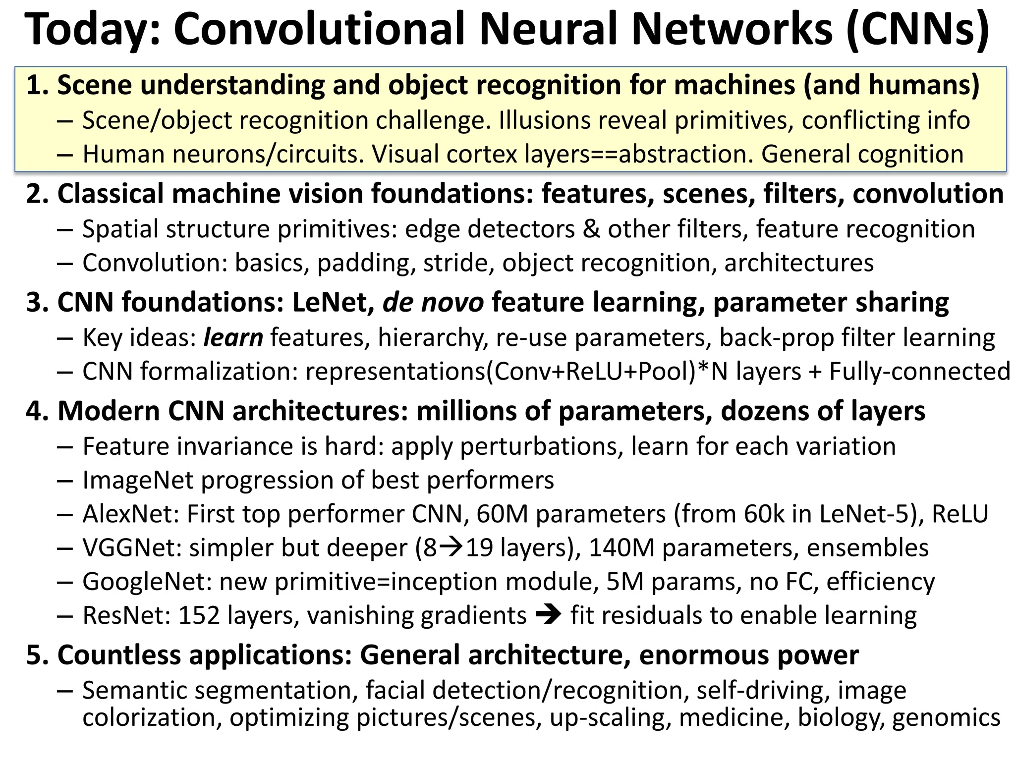
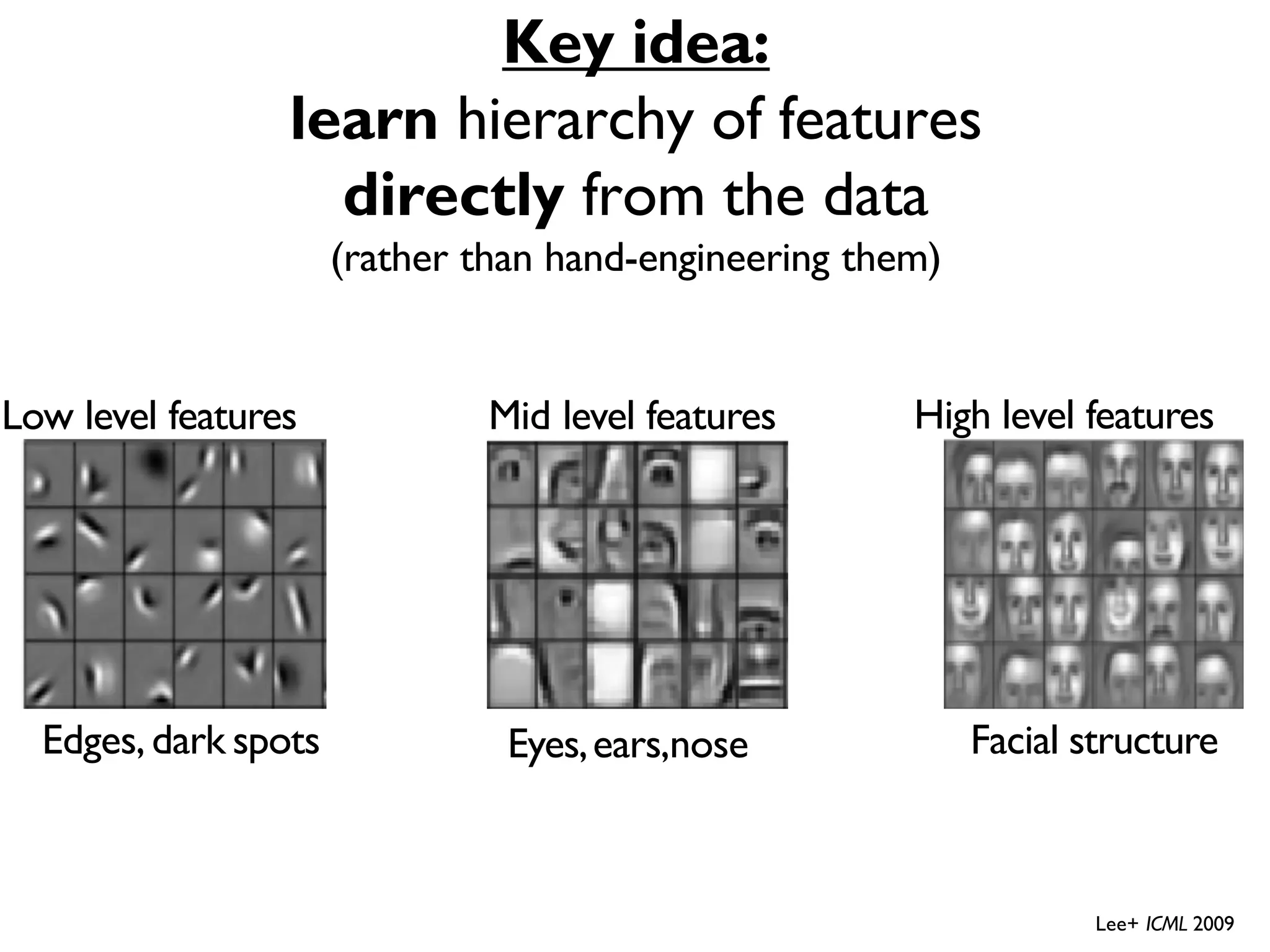
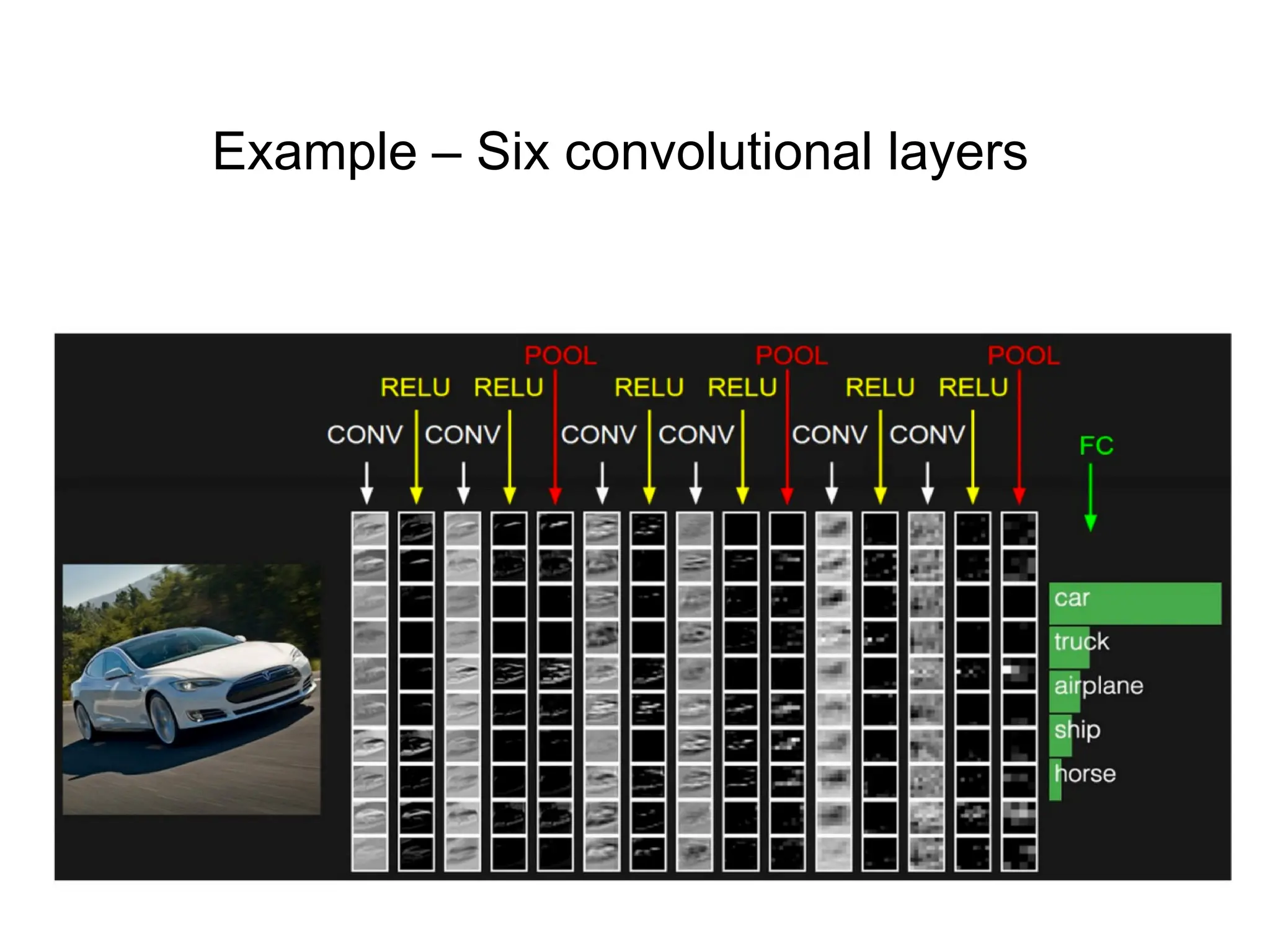
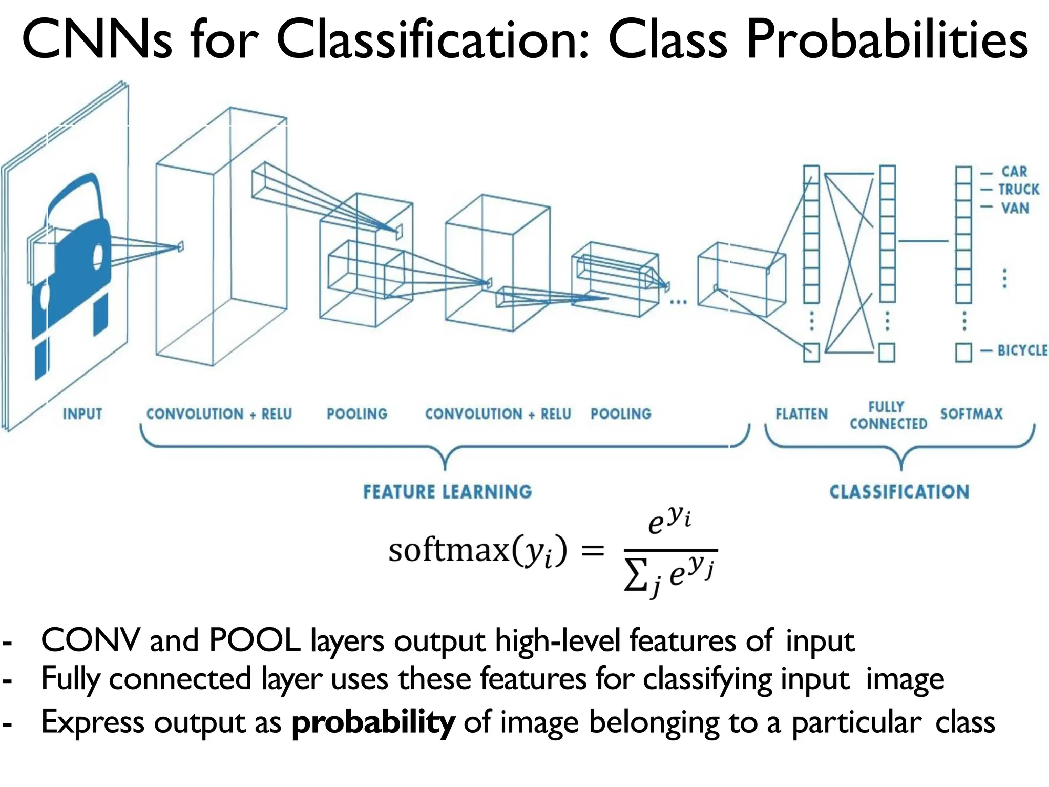
![What computers ‘see’: Images as Numbers What the computer "sees" Levin Image Processing & Computer Vision An image is just a matrix of numbers [0,255].i.e.,1080x1080x3 for an RGB image. Question: is this Lincoln?Washington? Jefferson? Obama? How can the computer answer this question? What you see Input Image Input Image + values Pixel intensity values (“pix-el”=picture-element) What you both see Can I just do classification on the 1,166400-long image vector directly? No. Instead: exploit image spatial structure. Learn patches. Build them up](https://image.slidesharecdn.com/l03cnnsmk2-231007032320-a43fab35/75/CNN-Algorithm-6-2048.jpg)
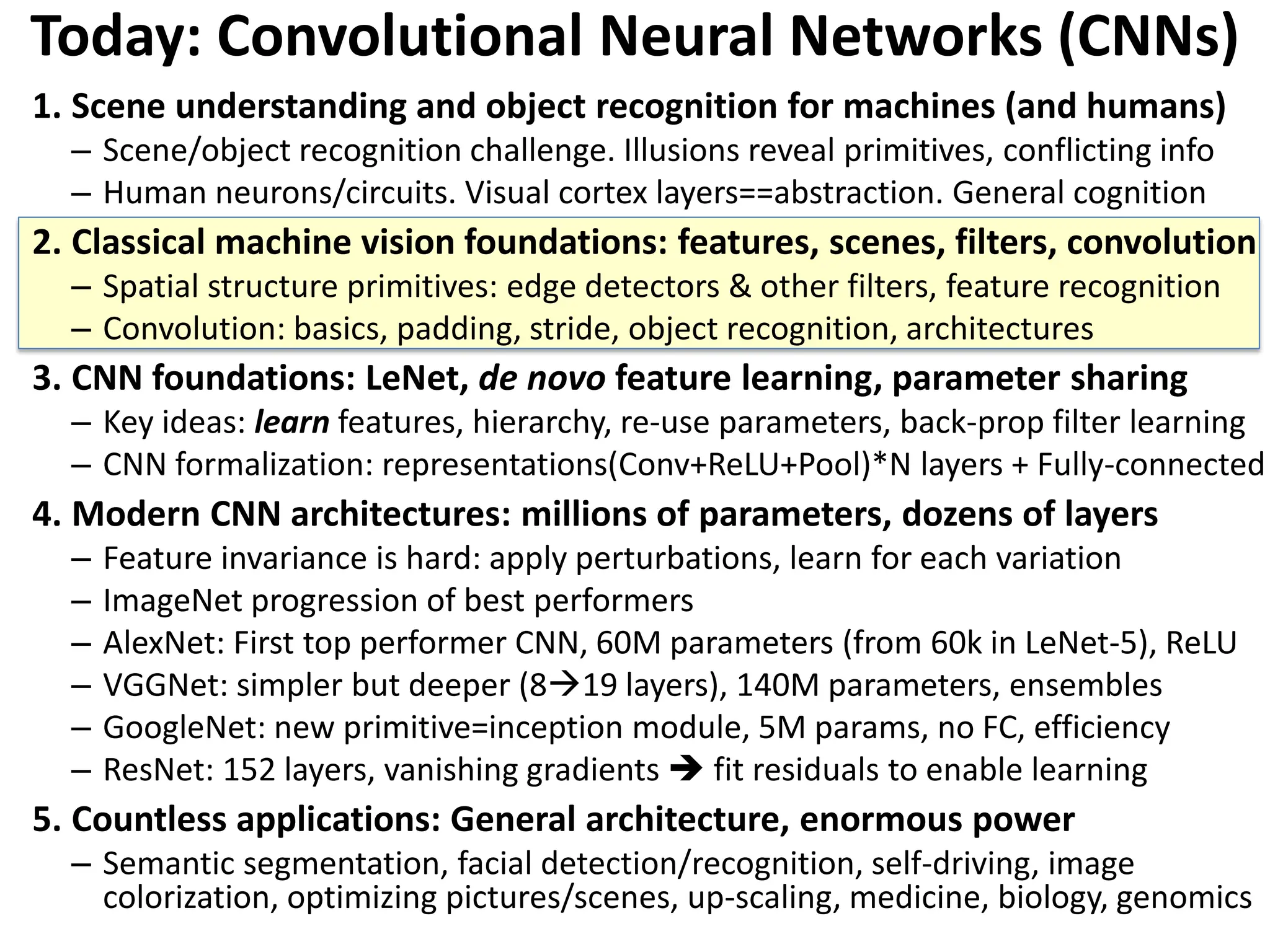
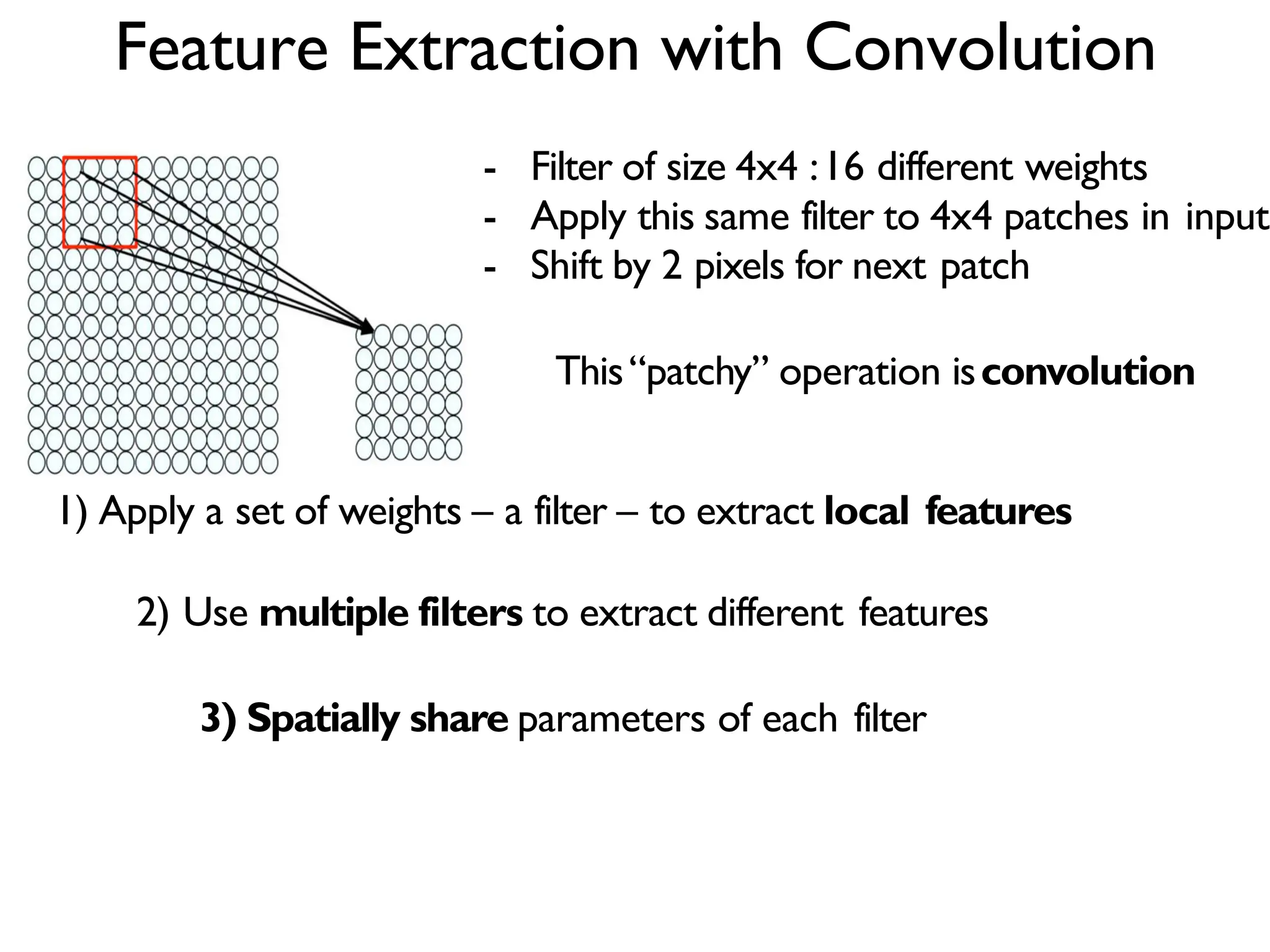
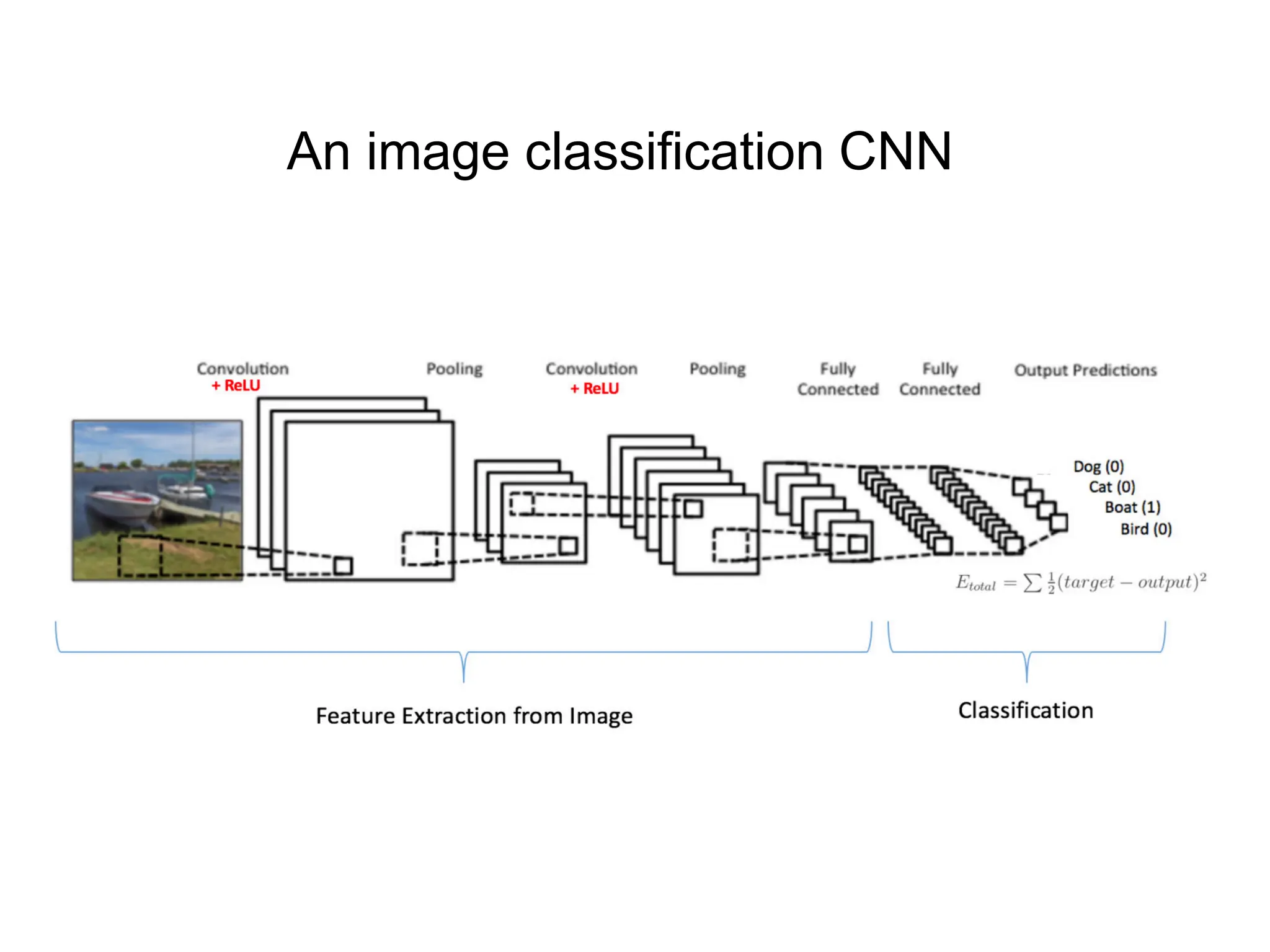
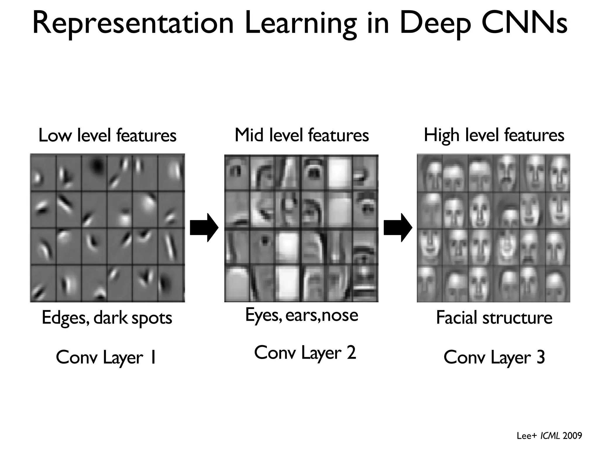
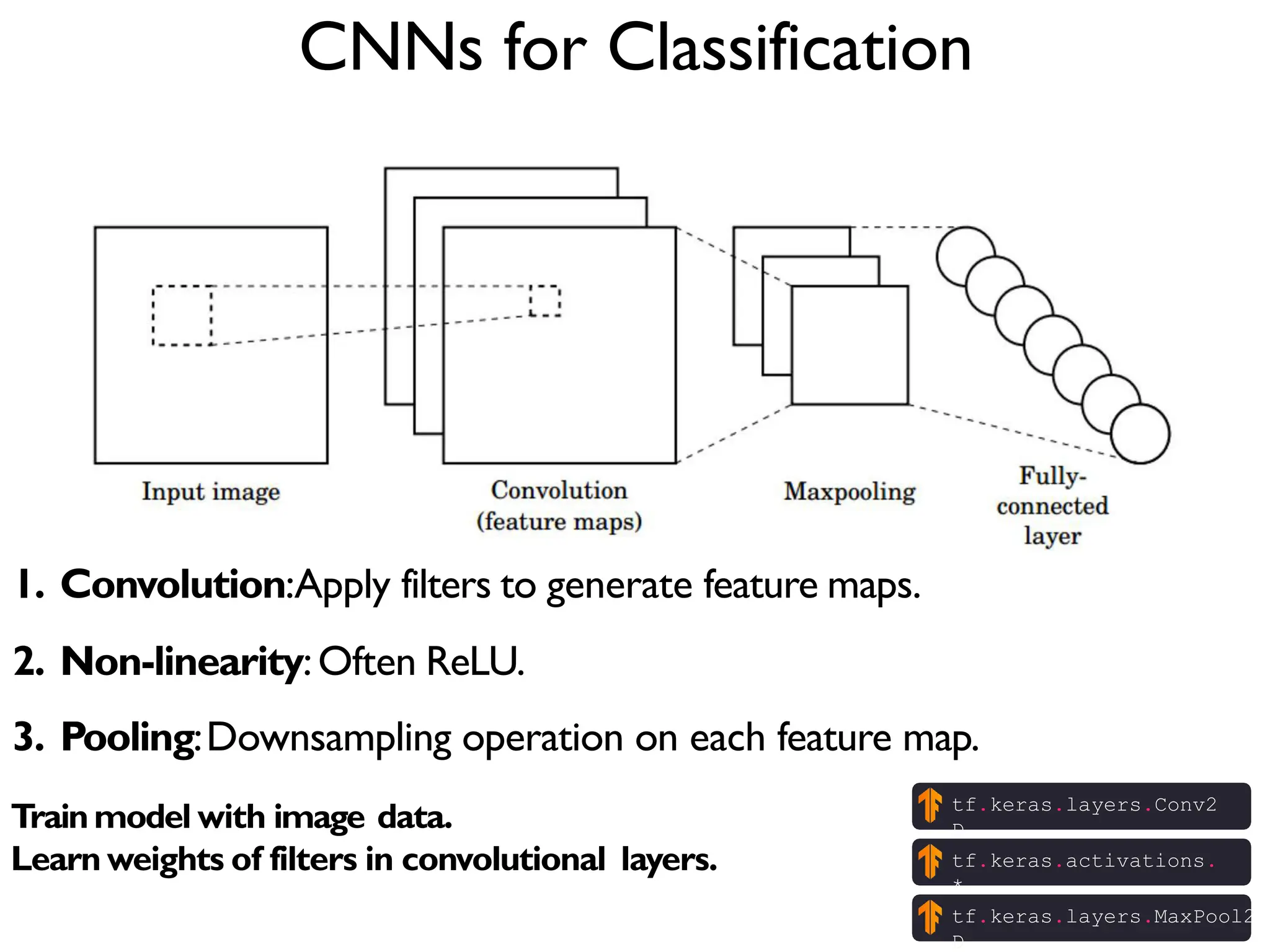
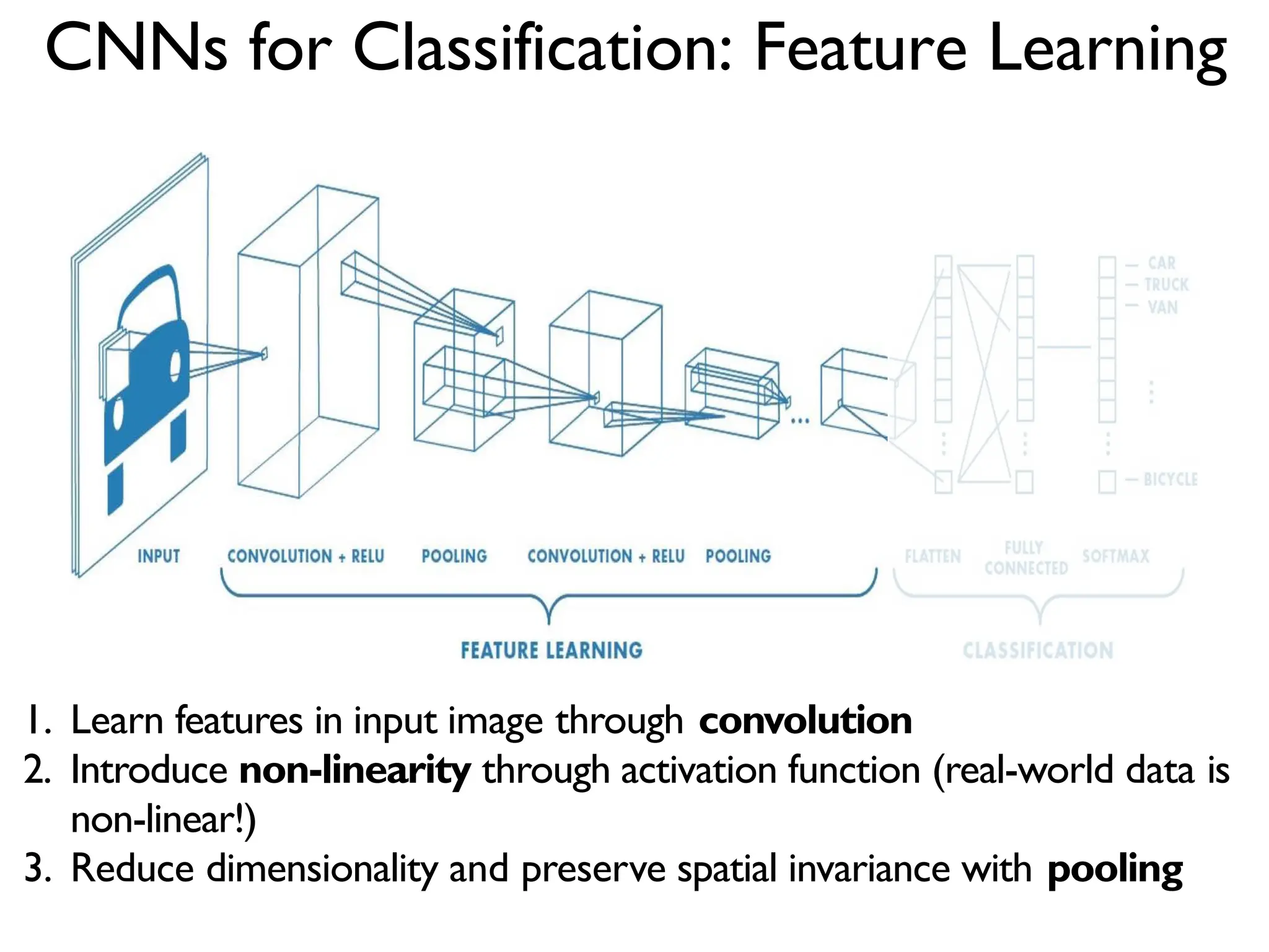
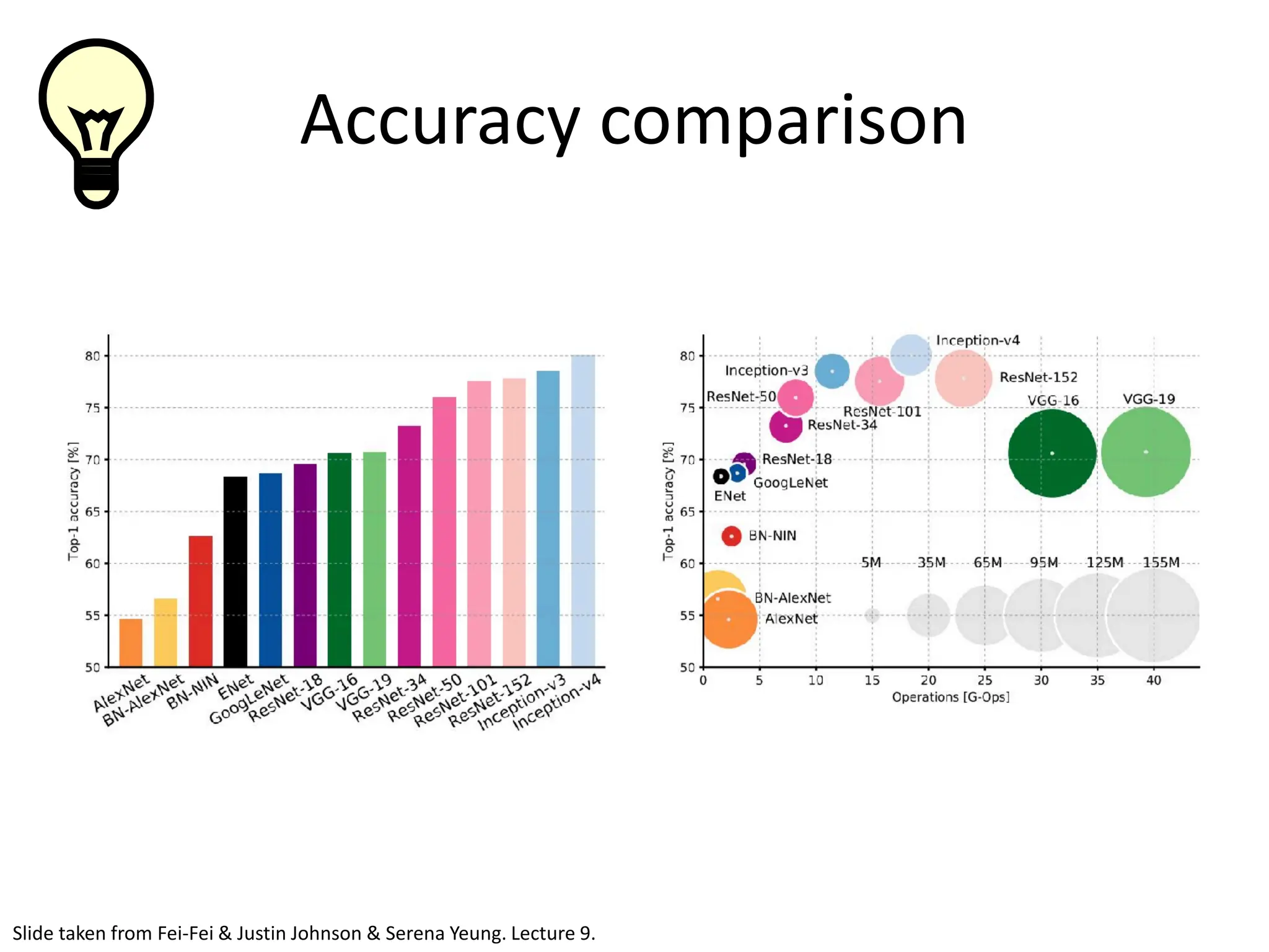
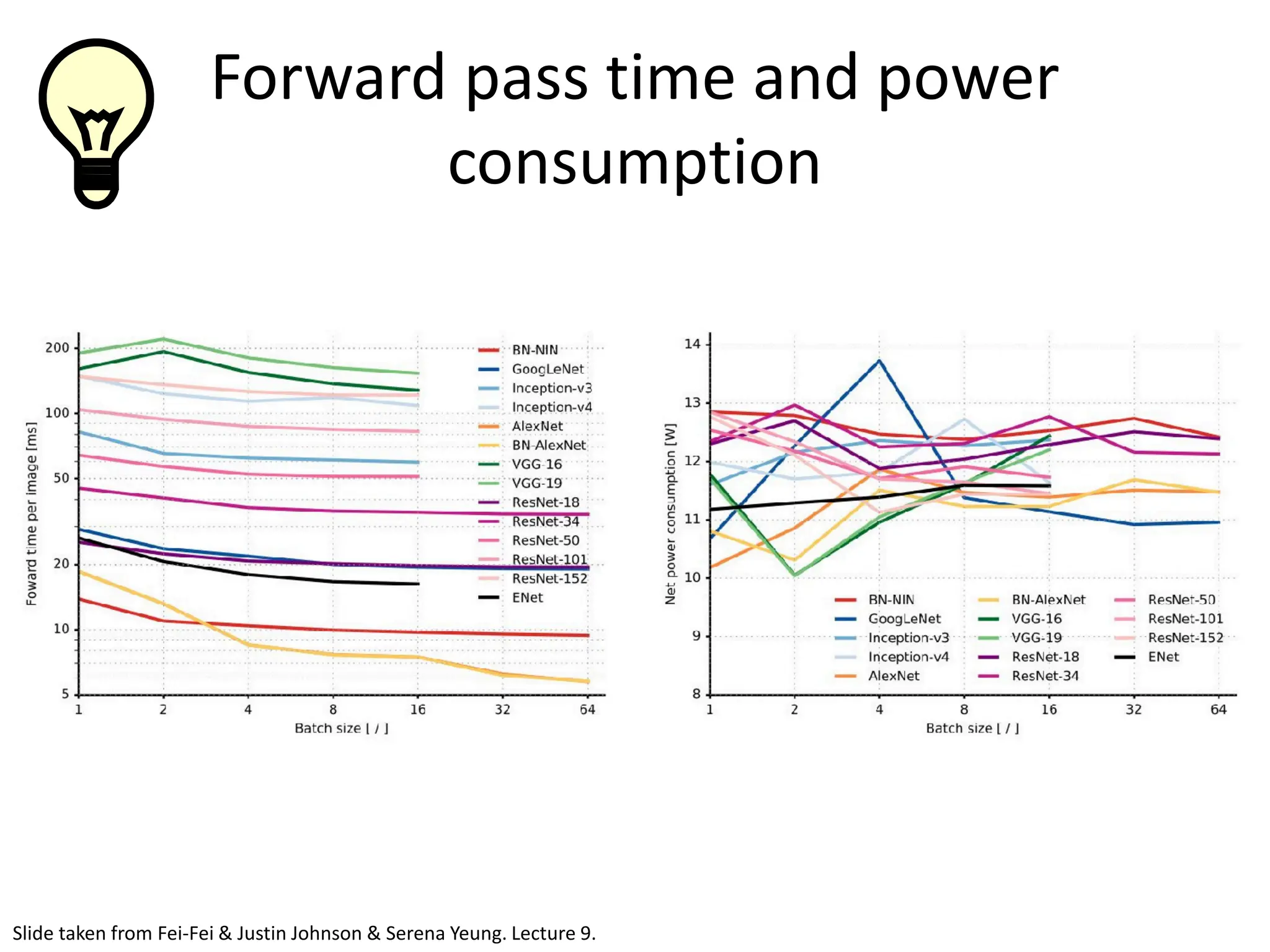
![(Goodfellow 2016) Zero Padding Controls Output Size • Full convolution: zero pad input so output is produced whenever an output value contains at least one input value (expands output) • Valid-only convolution: output only when entire kernel contained in input (shrinks output) • Same convolution: zero pad input so output is same size as input dimensions x = tf.nn.conv2d(x, W, strides=[1,strides,strides,1],padding='SAME') • TF convolution operator takes stride and zero fill option as parameters • Stride is distance between kernel applications in each dimension • Padding can be SAME or VALID](https://image.slidesharecdn.com/l03cnnsmk2-231007032320-a43fab35/75/CNN-Algorithm-27-2048.jpg)


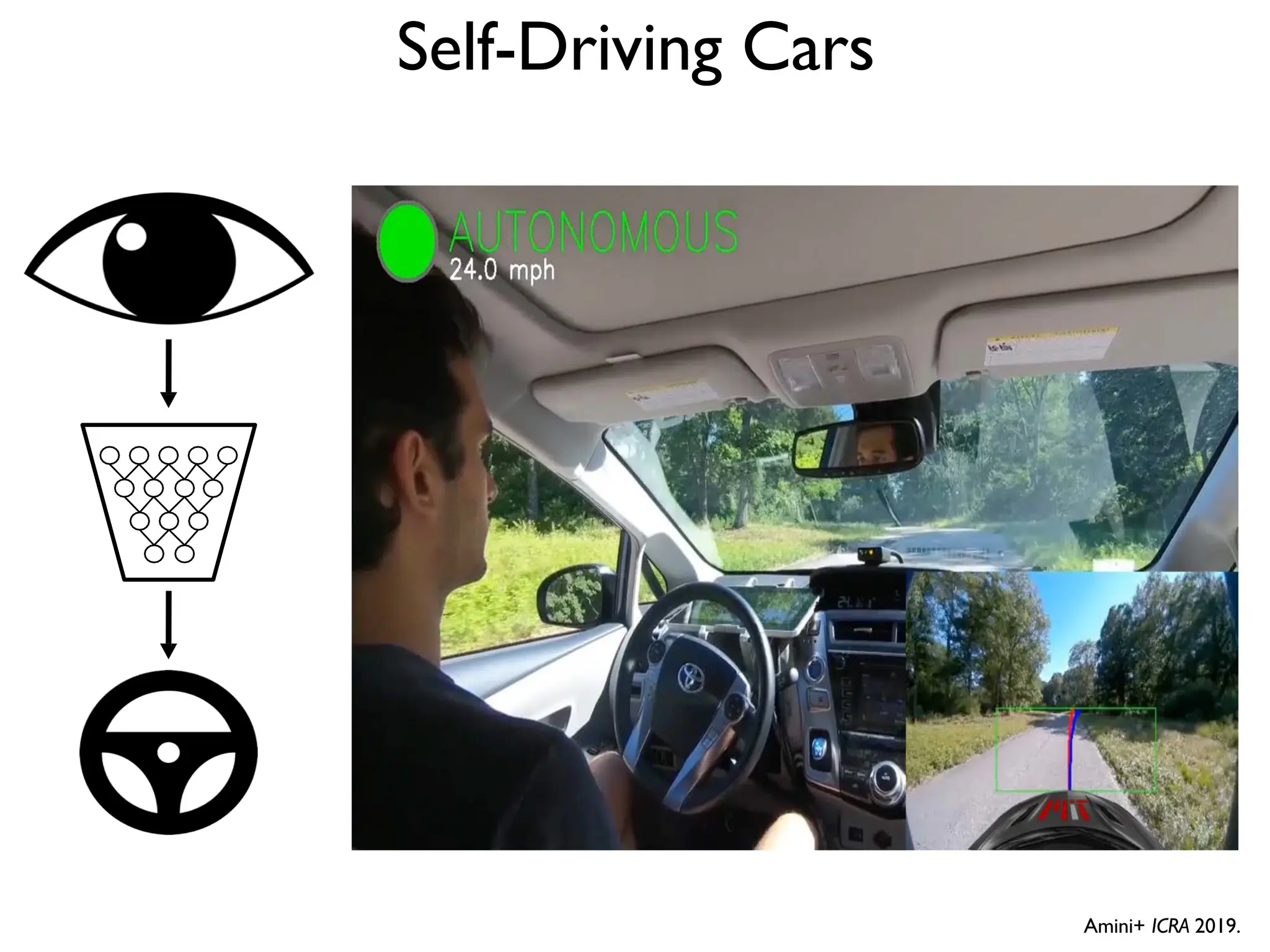
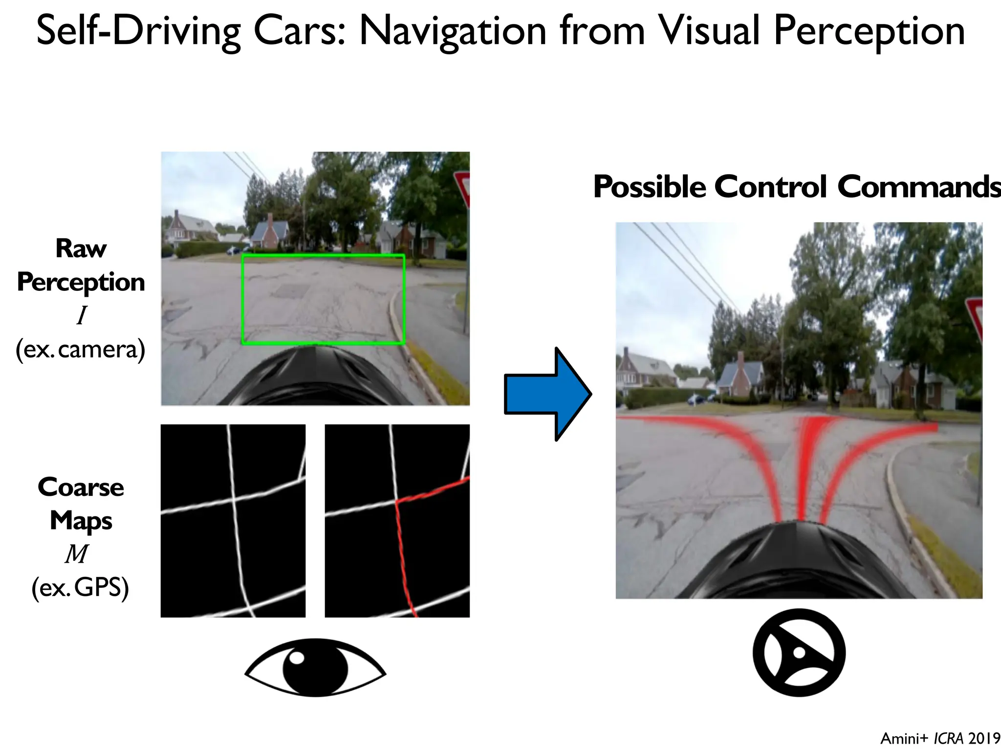
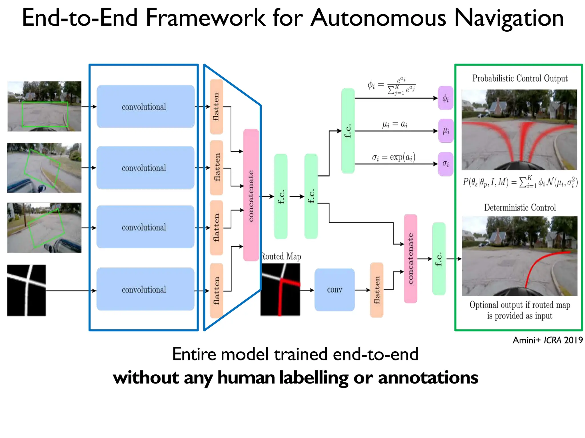
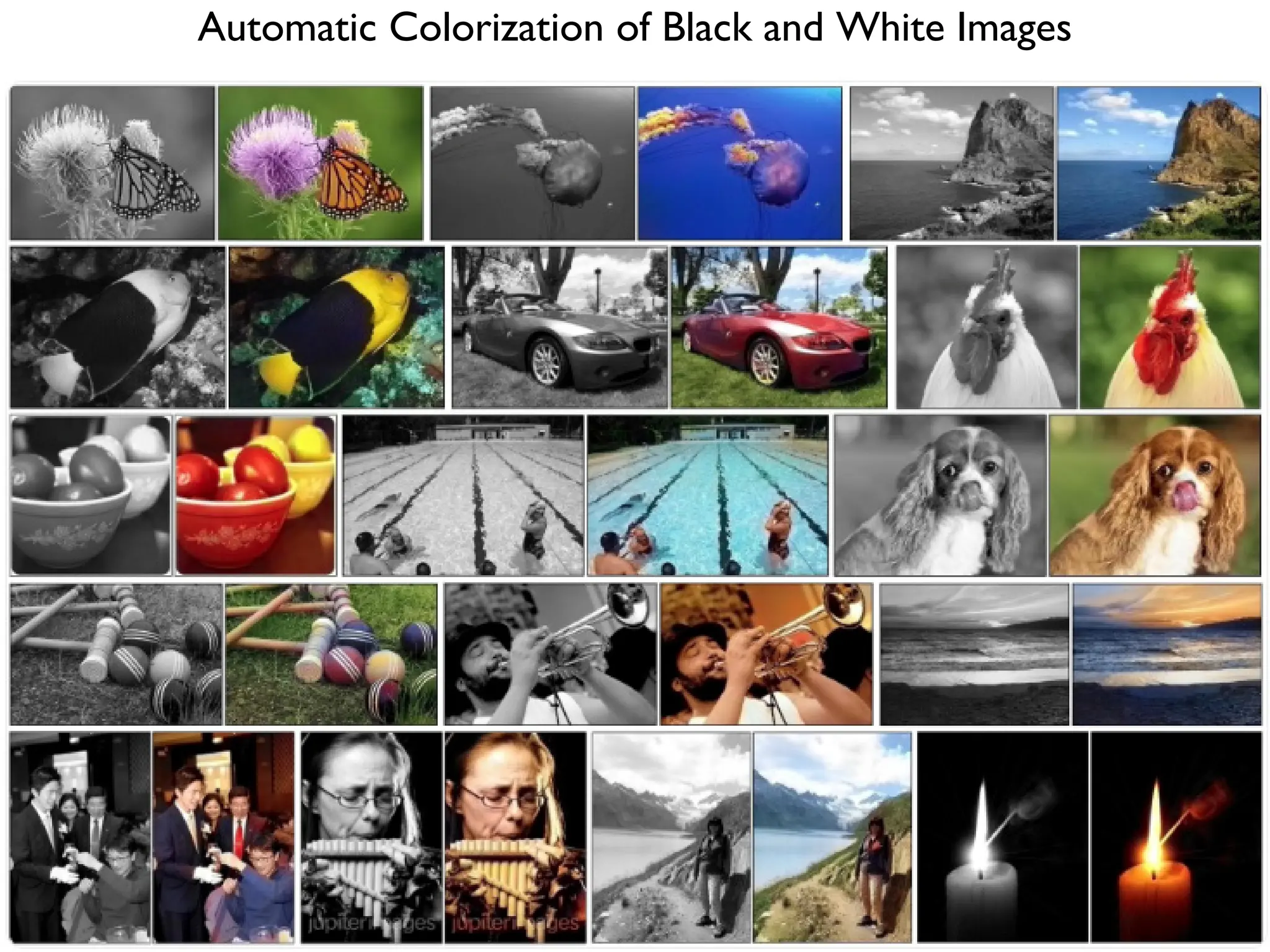
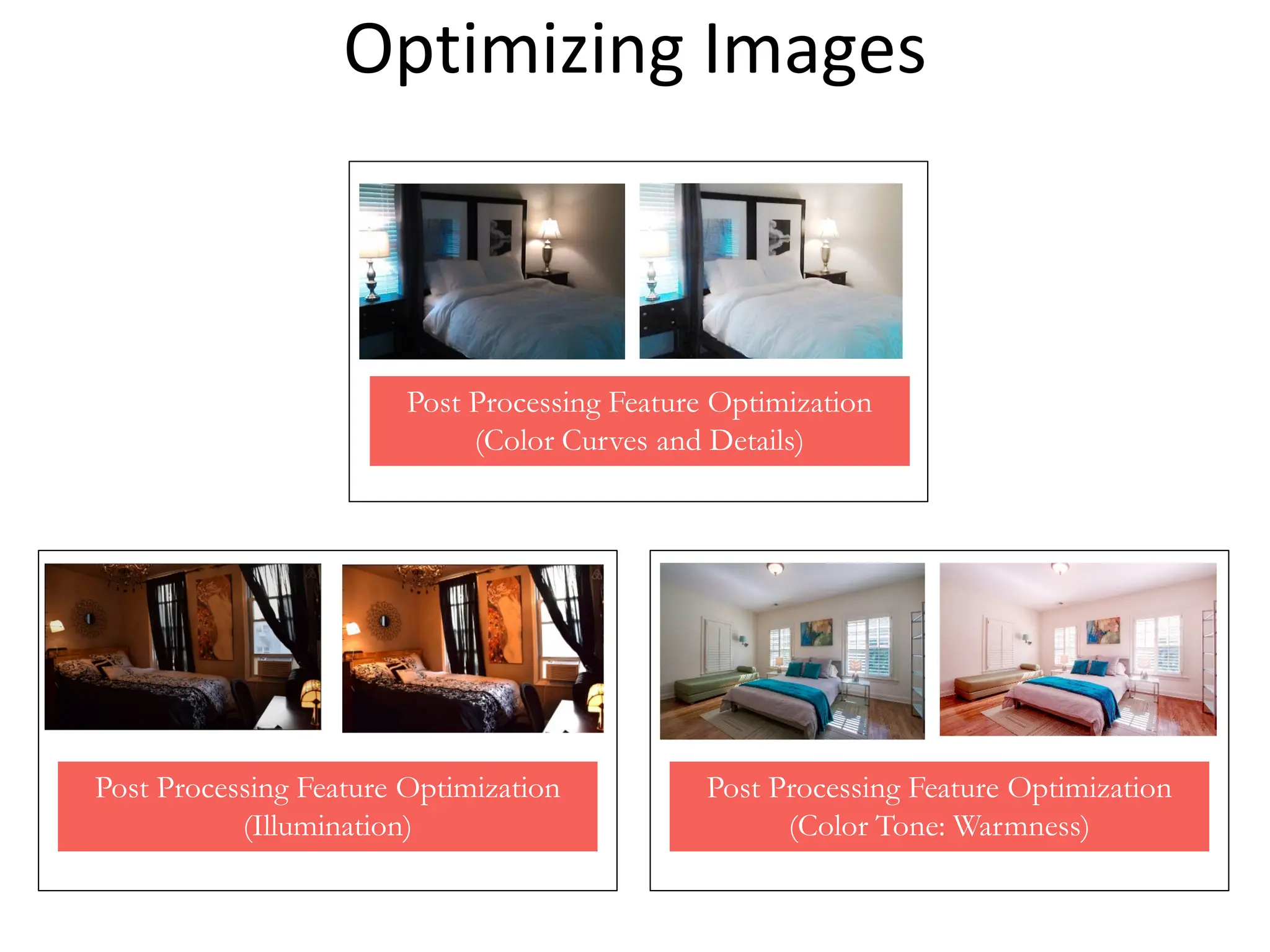
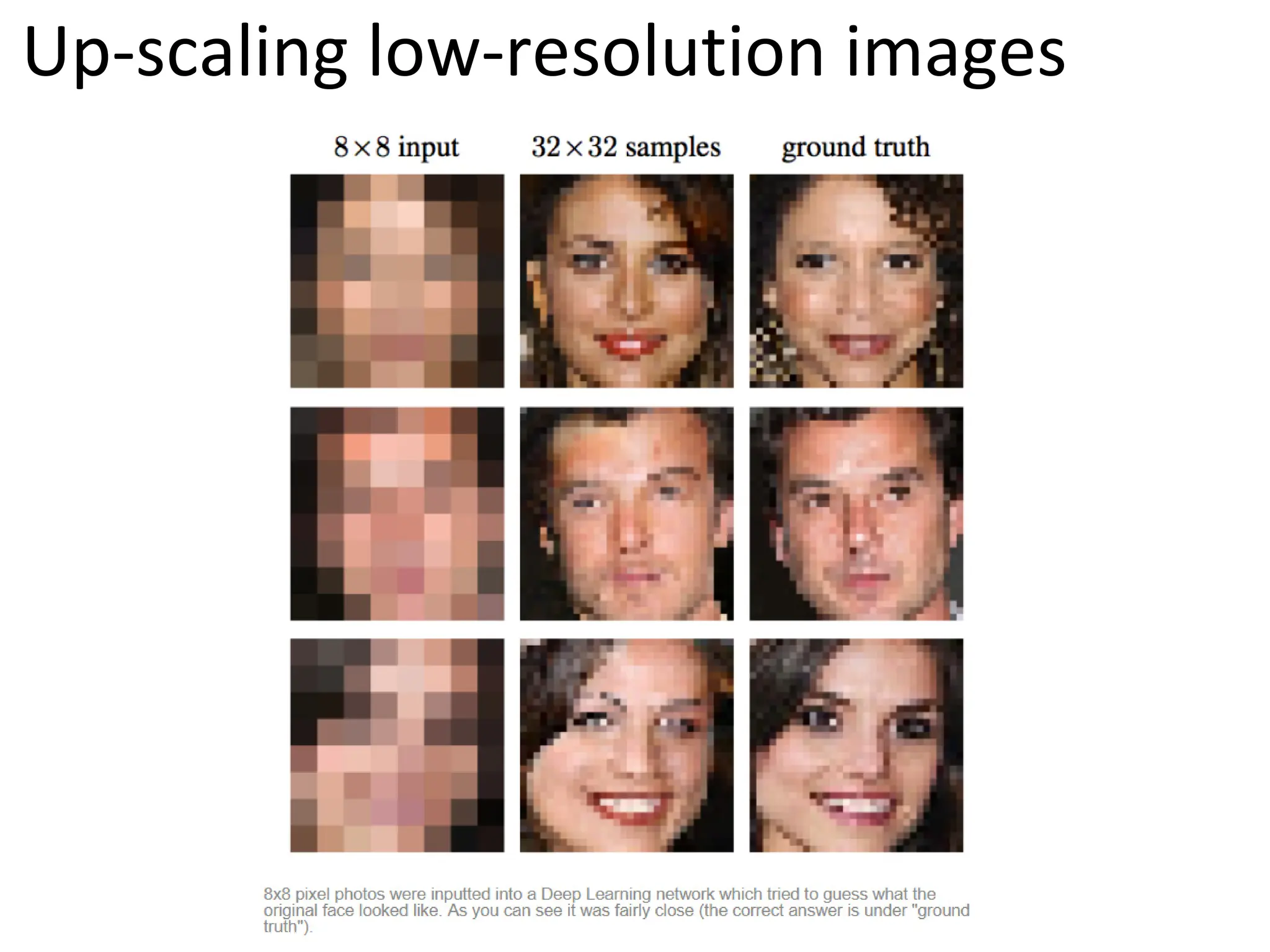
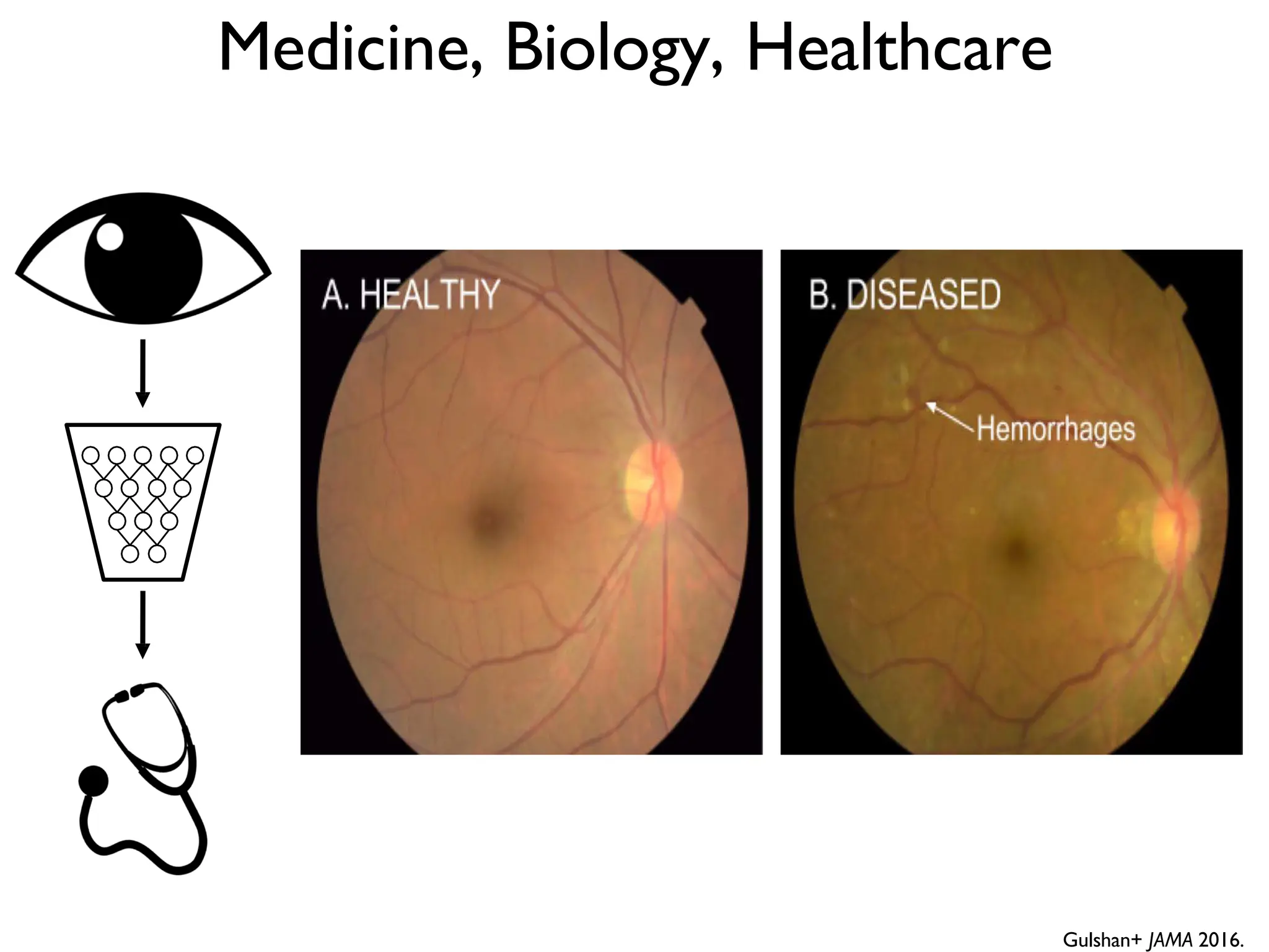
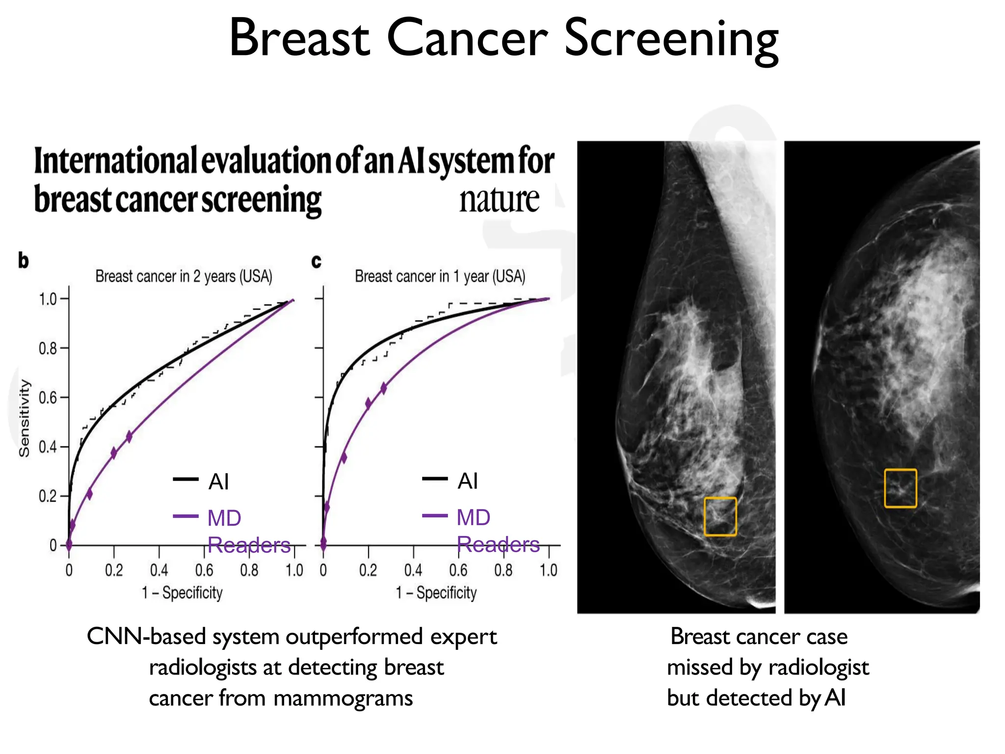
![LeNet-5 • Gradient Based Learning Applied To Document Recognition - Y. Lecun, L. Bottou, Y. Bengio, P. Haffner; 1998 • Helped establish how we use CNNs today • Replaced manual feature extraction [LeCun et al., 1998]](https://image.slidesharecdn.com/l03cnnsmk2-231007032320-a43fab35/75/CNN-Algorithm-34-2048.jpg)
![LeNet-5 ⋮ ⋮ � 𝑦𝑦 32×32×1 28×28×6 14×14×6 10×10×16 5×5×16 120 84 5 × 5 s = 1 f = 2 s = 2 avg pool 5 × 5 s = 1 avg pool f = 2 s = 2 . . . . . . Reminder: Output size = (N+2P-F)/stride + 1 10 conv conv FC FC [LeCun et al., 1998] This slide is taken from Andrew Ng](https://image.slidesharecdn.com/l03cnnsmk2-231007032320-a43fab35/75/CNN-Algorithm-35-2048.jpg)
![LeNet-5 • Only 60K parameters • As we go deeper in the network: 𝑁𝑁𝐻𝐻 ↓, 𝑁𝑁𝑊𝑊↓, 𝑁𝑁𝐶𝐶 ↑ • General structure: conv->pool->conv->pool->FC->FC->output • Different filters look at different channels • Sigmoid and Tanh nonlinearity [LeCun et al., 1998]](https://image.slidesharecdn.com/l03cnnsmk2-231007032320-a43fab35/75/CNN-Algorithm-36-2048.jpg)
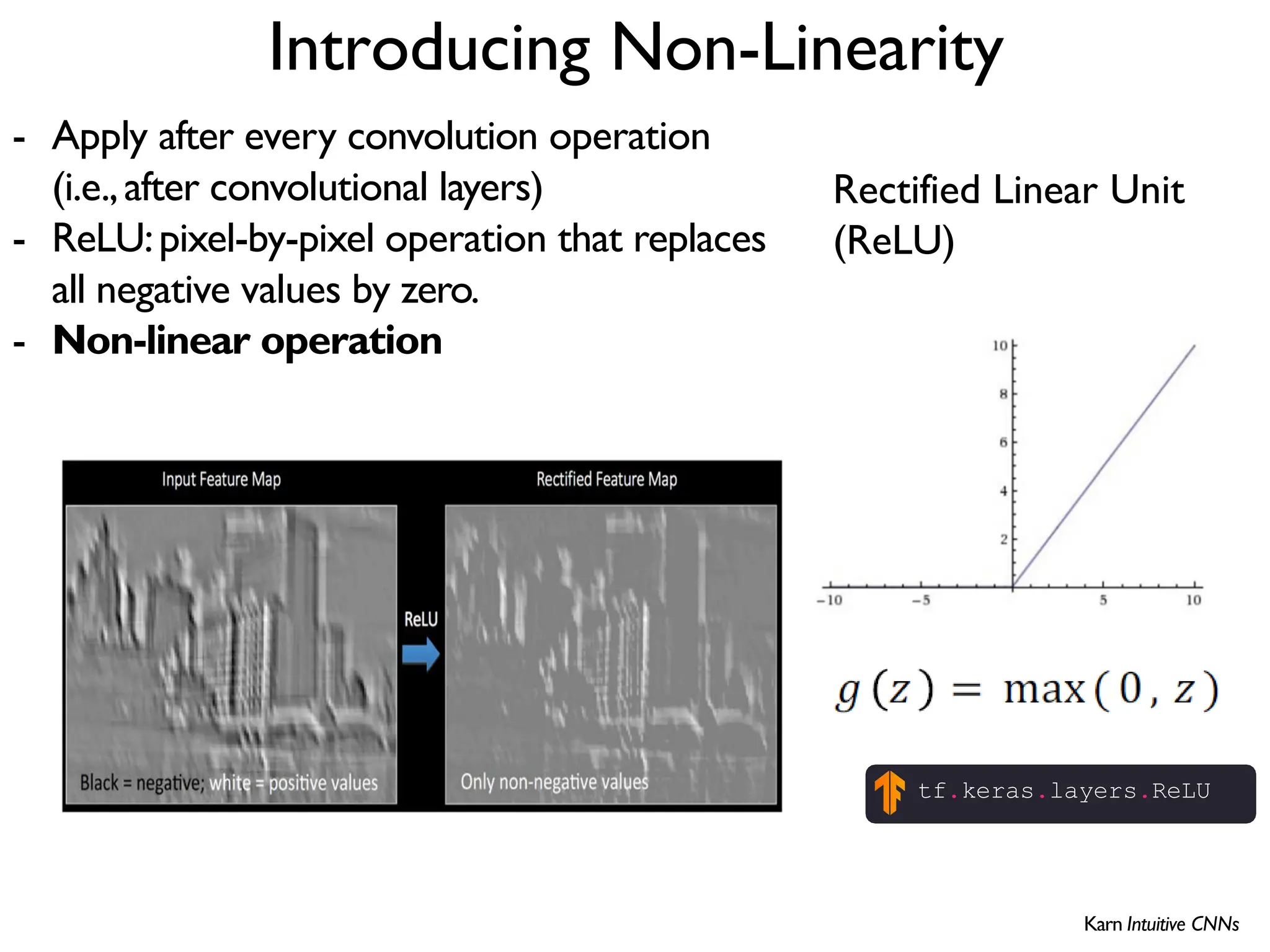
![The REctified Linear Unit (RELU) is a common non-linear detector stage after convolution x = tf.nn.conv2d(x, W, strides=[1, strides, strides, 1], padding='SAME') x = tf.nn.bias_add(x, b) x= tf.nn.relu(x) f(x) = max(0, x) When will we backpropagate through this? Once it “dies” what happens to it?](https://image.slidesharecdn.com/l03cnnsmk2-231007032320-a43fab35/75/CNN-Algorithm-48-2048.jpg)
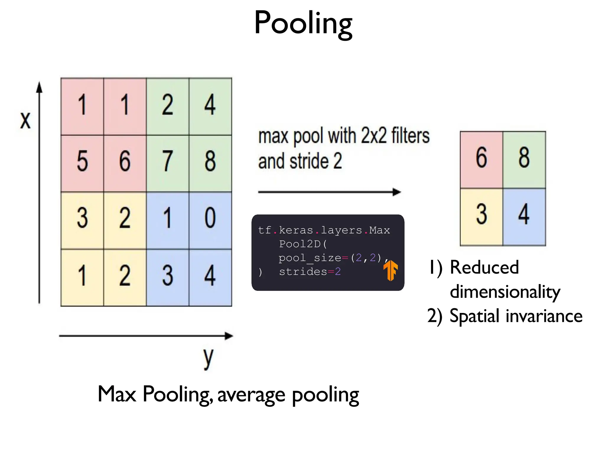
![Pooling reduces dimensionality by giving up spatial location • max pooling reports the maximum output within a defined neighborhood • Padding can be SAME or VALID x = tf.nn.max_pool(x, ksize=[1, k, k, 1], strides=[1, k, k, 1], padding='SAME') Output Input Pooling Batch H W Input channel Neighborhood [batch, height, width, channels]](https://image.slidesharecdn.com/l03cnnsmk2-231007032320-a43fab35/75/CNN-Algorithm-49-2048.jpg)
![Putting it all together import tensorflow as tf def generate_model(): model = tf.keras.Sequential([ # first convolutional layer tf.keras.layers.Conv2D(32, filter_size=3, activation='relu’), tf.keras.layers.MaxPool2D(pool_size=2, strides=2), # second convolutional layer tf.keras.layers.Conv2D(64, filter_size=3, activation='relu’), tf.keras.layers.MaxPool2D(pool_size=2, strides=2), # fully connected classifier tf.keras.layers.Flatten(), tf.keras.layers.Dense(1024, activation='relu’), tf.keras.layers.Dense(10, activation=‘softmax’) # 10 outputs ]) return model](https://image.slidesharecdn.com/l03cnnsmk2-231007032320-a43fab35/75/CNN-Algorithm-53-2048.jpg)
![LeNet-5 • Gradient Based Learning Applied To Document Recognition - Y. Lecun, L. Bottou, Y. Bengio, P. Haffner; 1998 • Helped establish how we use CNNs today • Replaced manual feature extraction [LeCun et al., 1998]](https://image.slidesharecdn.com/l03cnnsmk2-231007032320-a43fab35/75/CNN-Algorithm-60-2048.jpg)
![AlexNet • ImageNet Classification with Deep Convolutional Neural Networks - Alex Krizhevsky, Ilya Sutskever, Geoffrey E. Hinton; 2012 • Facilitated by GPUs, highly optimized convolution implementation and large datasets (ImageNet) • One of the largest CNNs to date • Has 60 Million parameter compared to 60k parameter of LeNet-5 [Krizhevsky et al., 2012]](https://image.slidesharecdn.com/l03cnnsmk2-231007032320-a43fab35/75/CNN-Algorithm-62-2048.jpg)

![AlexNet [Krizhevsky et al., 2012] Architecture CONV1 MAX POOL1 NORM1 CONV2 MAX POOL2 NORM2 CONV3 CONV4 CONV5 Max POOL3 FC6 FC7 FC8 • Input: 227x227x3 images (224x224 before padding) • First layer: 96 11x11 filters applied at stride 4 • Output volume size? (N-F)/s+1 = (227-11)/4+1 = 55 -> [55x55x96] • Number of parameters in this layer? (11*11*3)*96 = 35K Slide taken from Fei-Fei & Justin Johnson & Serena Yeung. Lecture 9.](https://image.slidesharecdn.com/l03cnnsmk2-231007032320-a43fab35/75/CNN-Algorithm-65-2048.jpg)
![AlexNet [Krizhevsky et al., 2012]](https://image.slidesharecdn.com/l03cnnsmk2-231007032320-a43fab35/75/CNN-Algorithm-66-2048.jpg)
![AlexNet [Krizhevsky et al., 2012] • Input: 227x227x3 images (224x224 before padding) • After CONV1: 55x55x96 • Second layer: 3x3 filters applied at stride 2 • Output volume size? (N-F)/s+1 = (55-3)/2+1 = 27 -> [27x27x96] • Number of parameters in this layer? 0! Slide taken from Fei-Fei & Justin Johnson & Serena Yeung. Lecture 9. Architecture CONV1 MAX POOL1 NORM1 CONV2 MAX POOL2 NORM2 CONV3 CONV4 CONV5 Max POOL3 FC6 FC7 FC8](https://image.slidesharecdn.com/l03cnnsmk2-231007032320-a43fab35/75/CNN-Algorithm-67-2048.jpg)
![AlexNet . . . 227×227 ×3 55×55 × 96 27×27 ×96 27×27 ×256 13×13 ×256 13×13 ×384 13×13 ×384 13×13 ×256 6×6 ×256 11 × 11 s = 4 P = 0 3 × 3 s = 2 max pool 5 × 5 S = 1 P = 2 3 × 3 s = 2 max pool 3 × 3 S = 1 P = 1 3 × 3 s = 1 P = 1 3 × 3 S = 1 P = 1 3 × 3 s = 2 max pool conv conv conv conv conv . . . [Krizhevsky et al., 2012] . . . This slide is taken from Andrew Ng](https://image.slidesharecdn.com/l03cnnsmk2-231007032320-a43fab35/75/CNN-Algorithm-68-2048.jpg)
![AlexNet . . . 4096 4096 Softmax 1000 ⋮ ⋮ [Krizhevsky et al., 2012] FC FC This slide is taken from Andrew Ng](https://image.slidesharecdn.com/l03cnnsmk2-231007032320-a43fab35/75/CNN-Algorithm-69-2048.jpg)
![AlexNet [Krizhevsky et al., 2012] Details/Retrospectives: • first use of ReLU • used Norm layers (not common anymore) • heavy data augmentation • dropout 0.5 • batch size 128 • 7 CNN ensemble Slide taken from Fei-Fei & Justin Johnson & Serena Yeung. Lecture 9.](https://image.slidesharecdn.com/l03cnnsmk2-231007032320-a43fab35/75/CNN-Algorithm-70-2048.jpg)
![AlexNet [Krizhevsky et al., 2012] • Trained on GTX 580 GPU with only 3 GB of memory. • Network spread across 2 GPUs, half the neurons (feature maps) on each GPU. • CONV1, CONV2, CONV4, CONV5: Connections only with feature maps on same GPU. • CONV3, FC6, FC7, FC8: Connections with all feature maps in preceding layer, communication across GPUs. Slide taken from Fei-Fei & Justin Johnson & Serena Yeung. Lecture 9.](https://image.slidesharecdn.com/l03cnnsmk2-231007032320-a43fab35/75/CNN-Algorithm-71-2048.jpg)
![AlexNet AlexNet was the coming out party for CNNs in the computer vision community. This was the first time a model performed so well on a historically difficult ImageNet dataset. This paper illustrated the benefits of CNNs and backed them up with record breaking performance in the competition. [Krizhevsky et al., 2012]](https://image.slidesharecdn.com/l03cnnsmk2-231007032320-a43fab35/75/CNN-Algorithm-72-2048.jpg)
![VGGNet • Very Deep Convolutional Networks For Large Scale Image Recognition - Karen Simonyan and Andrew Zisserman; 2015 • The runner-up at the ILSVRC 2014 competition • Significantly deeper than AlexNet • 140 million parameters [Simonyan and Zisserman, 2014]](https://image.slidesharecdn.com/l03cnnsmk2-231007032320-a43fab35/75/CNN-Algorithm-75-2048.jpg)
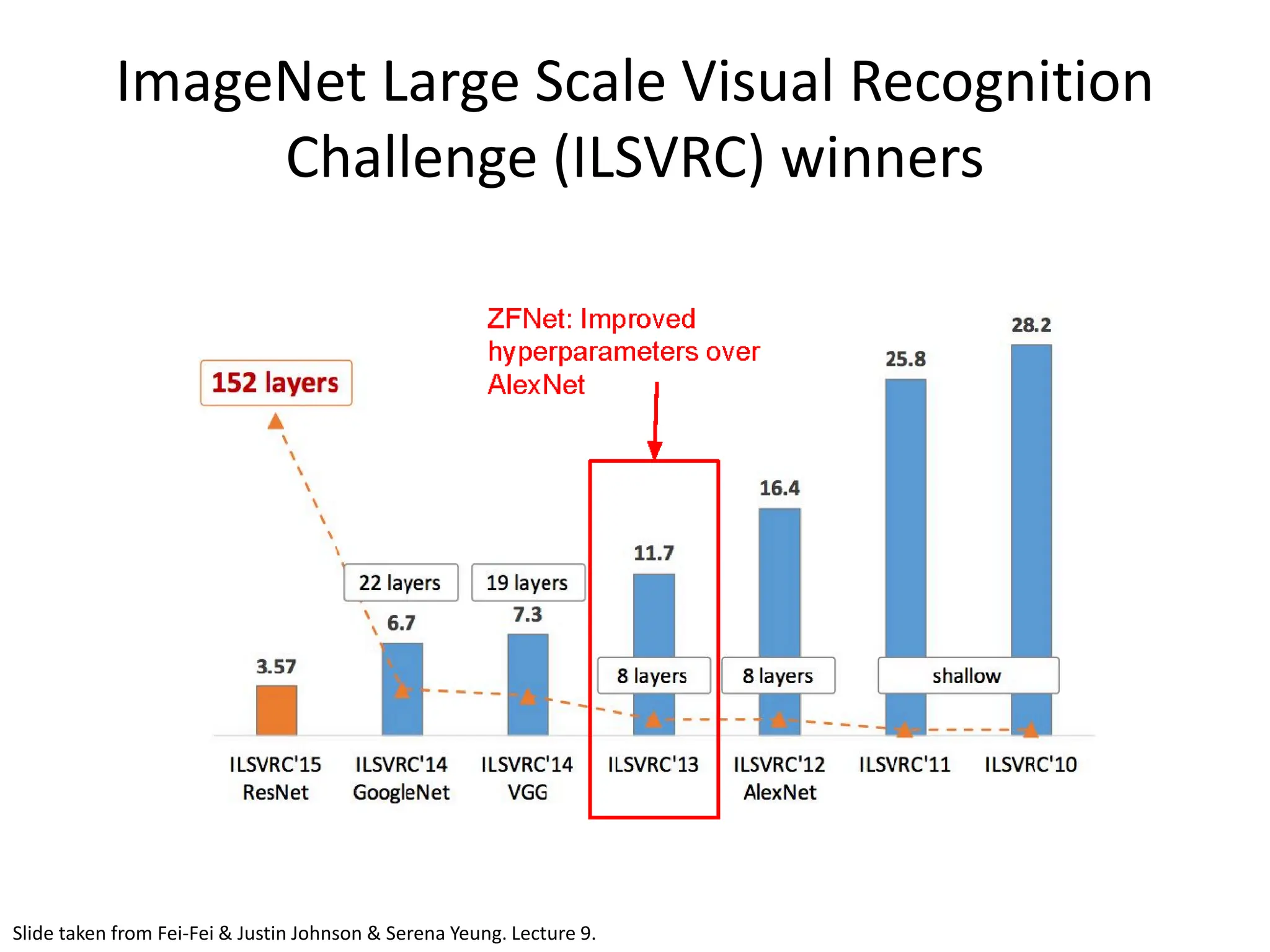
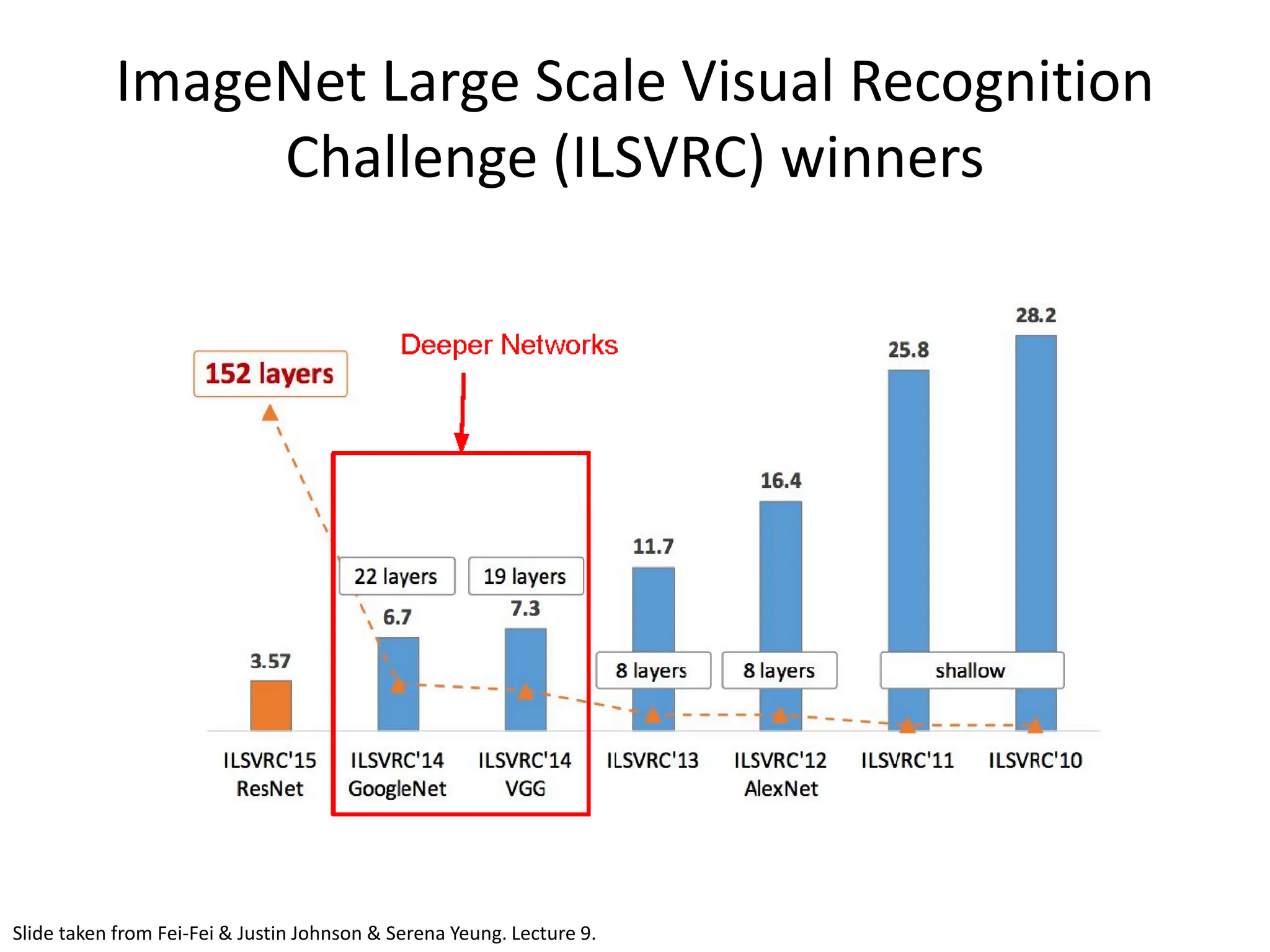
![VGGNet • Smaller filters Only 3x3 CONV filters, stride 1, pad 1 and 2x2 MAX POOL , stride 2 • Deeper network AlexNet: 8 layers VGGNet: 16 - 19 layers • ZFNet: 11.7% top 5 error in ILSVRC’13 • VGGNet: 7.3% top 5 error in ILSVRC’14 Slide taken from Fei-Fei & Justin Johnson & Serena Yeung. Lecture 9. [Simonyan and Zisserman, 2014] Input 3x3 conv, 64 3x3 conv, 64 Pool 1/2 3x3 conv, 128 3x3 conv, 128 Pool 1/2 3x3 conv, 256 3x3 conv, 256 Pool 1/2 3x3 conv, 512 3x3 conv, 512 3x3 conv, 512 Pool 1/2 3x3 conv, 512 3x3 conv, 512 3x3 conv, 512 Pool 1/2 FC 4096 FC 4096 FC 1000 Softmax](https://image.slidesharecdn.com/l03cnnsmk2-231007032320-a43fab35/75/CNN-Algorithm-76-2048.jpg)
![VGGNet [Simonyan and Zisserman, 2014] • Why use smaller filters? (3x3 conv) Stack of three 3x3 conv (stride 1) layers has the same effective receptive field as one 7x7 conv layer. • What is the effective receptive field of three 3x3 conv (stride 1) layers? 7x7 But deeper, more non-linearities And fewer parameters: 3 * (32C2) vs. 72C2 for C channels per layer Slide taken from Fei-Fei & Justin Johnson & Serena Yeung. Lecture 9.](https://image.slidesharecdn.com/l03cnnsmk2-231007032320-a43fab35/75/CNN-Algorithm-77-2048.jpg)
![VGGNet [Simonyan and Zisserman, 2014] VGG16: TOTAL memory: 24M * 4 bytes ~= 96MB / image TOTAL params: 138M parameters Slide taken from Fei-Fei & Justin Johnson & Serena Yeung. Lecture 9. Input 3x3 conv, 64 3x3 conv, 64 Pool 3x3 conv, 128 3x3 conv, 128 Pool 3x3 conv, 256 3x3 conv, 256 3x3 conv, 256 Pool 3x3 conv, 512 3x3 conv, 512 3x3 conv, 512 Pool 3x3 conv, 512 3x3 conv, 512 3x3 conv, 512 Pool FC 4096 FC 4096 FC 1000 Softmax](https://image.slidesharecdn.com/l03cnnsmk2-231007032320-a43fab35/75/CNN-Algorithm-78-2048.jpg)
![[Simonyan and Zisserman, 2014] Slide taken from Fei-Fei & Justin Johnson & Serena Yeung. Lecture 9. Input memory: 224*224*3=150K params: 0 3x3 conv, 64 memory: 224*224*64=3.2M params: (3*3*3)*64 = 1,728 3x3 conv, 64 memory: 224*224*64=3.2M params: (3*3*64)*64 = 36,864 Pool memory: 112*112*64=800K params: 0 3x3 conv, 128 memory: 112*112*128=1.6M params: (3*3*64)*128 = 73,728 3x3 conv, 128 memory: 112*112*128=1.6M params: (3*3*128)*128 = 147,456 Pool memory: 56*56*128=400K params: 0 3x3 conv, 256 memory: 56*56*256=800K params: (3*3*128)*256 = 294,912 3x3 conv, 256 memory: 56*56*256=800K params: (3*3*256)*256 = 589,824 3x3 conv, 256 memory: 56*56*256=800K params: (3*3*256)*256 = 589,824 Pool memory: 28*28*256=200K params: 0 3x3 conv, 512 memory: 28*28*512=400K params: (3*3*256)*512 = 1,179,648 3x3 conv, 512 memory: 28*28*512=400K params: (3*3*512)*512 = 2,359,296 3x3 conv, 512 memory: 28*28*512=400K params: (3*3*512)*512 = 2,359,296 Pool memory: 14*14*512=100K params: 0 3x3 conv, 512 memory: 14*14*512=100K params: (3*3*512)*512 = 2,359,296 3x3 conv, 512 memory: 14*14*512=100K params: (3*3*512)*512 = 2,359,296 3x3 conv, 512 memory: 14*14*512=100K params: (3*3*512)*512 = 2,359,296 Pool memory: 7*7*512=25K params: 0 FC 4096 memory: 4096 params: 7*7*512*4096 = 102,760,448 FC 4096 memory: 4096 params: 4096*4096 = 16,777,216 FC 1000 memory: 1000 params: 4096*1000 = 4,096,000](https://image.slidesharecdn.com/l03cnnsmk2-231007032320-a43fab35/75/CNN-Algorithm-79-2048.jpg)
![VGGNet [Simonyan and Zisserman, 2014] Details/Retrospectives : • ILSVRC’14 2nd in classification, 1st in localization • Similar training procedure as AlexNet • No Local Response Normalisation (LRN) • Use VGG16 or VGG19 (VGG19 only slightly better, more memory) • Use ensembles for best results • FC7 features generalize well to other tasks • Trained on 4 Nvidia Titan Black GPUs for two to three weeks. Slide taken from Fei-Fei & Justin Johnson & Serena Yeung. Lecture 9.](https://image.slidesharecdn.com/l03cnnsmk2-231007032320-a43fab35/75/CNN-Algorithm-80-2048.jpg)
![VGGNet VGG Net reinforced the notion that convolutional neural networks have to have a deep network of layers in order for this hierarchical representation of visual data to work. Keep it deep. Keep it simple. [Simonyan and Zisserman, 2014]](https://image.slidesharecdn.com/l03cnnsmk2-231007032320-a43fab35/75/CNN-Algorithm-81-2048.jpg)

![GoogleNet • Going Deeper with Convolutions - Christian Szegedy et al.; 2015 • ILSVRC 2014 competition winner • Also significantly deeper than AlexNet • x12 less parameters than AlexNet • Focused on computational efficiency [Szegedy et al., 2014]](https://image.slidesharecdn.com/l03cnnsmk2-231007032320-a43fab35/75/CNN-Algorithm-83-2048.jpg)
![GoogleNet • 22 layers • Efficient “Inception” module - strayed from the general approach of simply stacking conv and pooling layers on top of each other in a sequential structure • No FC layers • Only 5 million parameters! • ILSVRC’14 classification winner (6.7% top 5 error) [Szegedy et al., 2014]](https://image.slidesharecdn.com/l03cnnsmk2-231007032320-a43fab35/75/CNN-Algorithm-84-2048.jpg)
![GoogleNet “Inception module”: design a good local network topology (network within a network) and then stack these modules on top of each other Slide taken from Fei-Fei & Justin Johnson & Serena Yeung. Lecture 9. [Szegedy et al., 2014] Filter concatenation Previous layer 1x1 convolution 3x3 convolution 5x5 convolution 1x1 convolution 1x1 convolution 1x1 convolution 3x3 max pooling](https://image.slidesharecdn.com/l03cnnsmk2-231007032320-a43fab35/75/CNN-Algorithm-85-2048.jpg)
![GoogleNet Details/Retrospectives : • Deeper networks, with computational efficiency • 22 layers • Efficient “Inception” module • No FC layers • 12x less params than AlexNet • ILSVRC’14 classification winner (6.7% top 5 error) Slide taken from Fei-Fei & Justin Johnson & Serena Yeung. Lecture 9. [Szegedy et al., 2014]](https://image.slidesharecdn.com/l03cnnsmk2-231007032320-a43fab35/75/CNN-Algorithm-86-2048.jpg)
![GoogleNet Introduced the idea that CNN layers didn’t always have to be stacked up sequentially. Coming up with the Inception module, the authors showed that a creative structuring of layers can lead to improved performance and computationally efficiency. [Szegedy et al., 2014]](https://image.slidesharecdn.com/l03cnnsmk2-231007032320-a43fab35/75/CNN-Algorithm-87-2048.jpg)
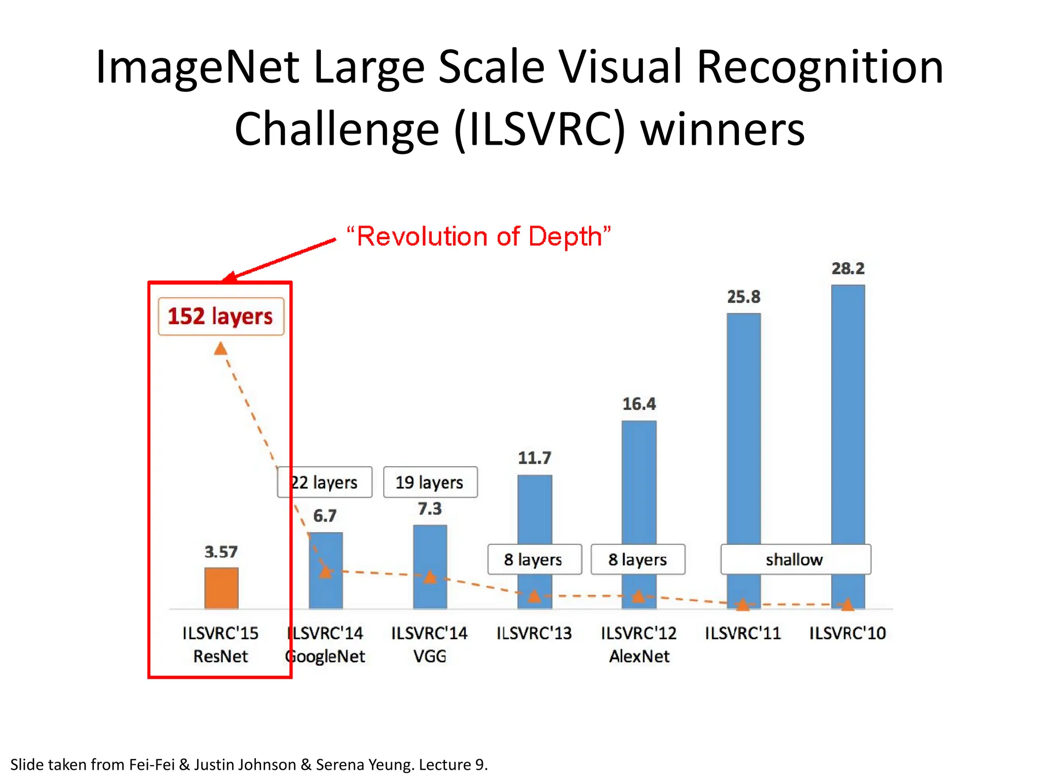
![ResNet • Deep Residual Learning for Image Recognition - Kaiming He, Xiangyu Zhang, Shaoqing Ren, Jian Sun; 2015 • Extremely deep network – 152 layers • Deeper neural networks are more difficult to train. • Deep networks suffer from vanishing and exploding gradients. • Present a residual learning framework to ease the training of networks that are substantially deeper than those used previously. [He et al., 2015]](https://image.slidesharecdn.com/l03cnnsmk2-231007032320-a43fab35/75/CNN-Algorithm-89-2048.jpg)
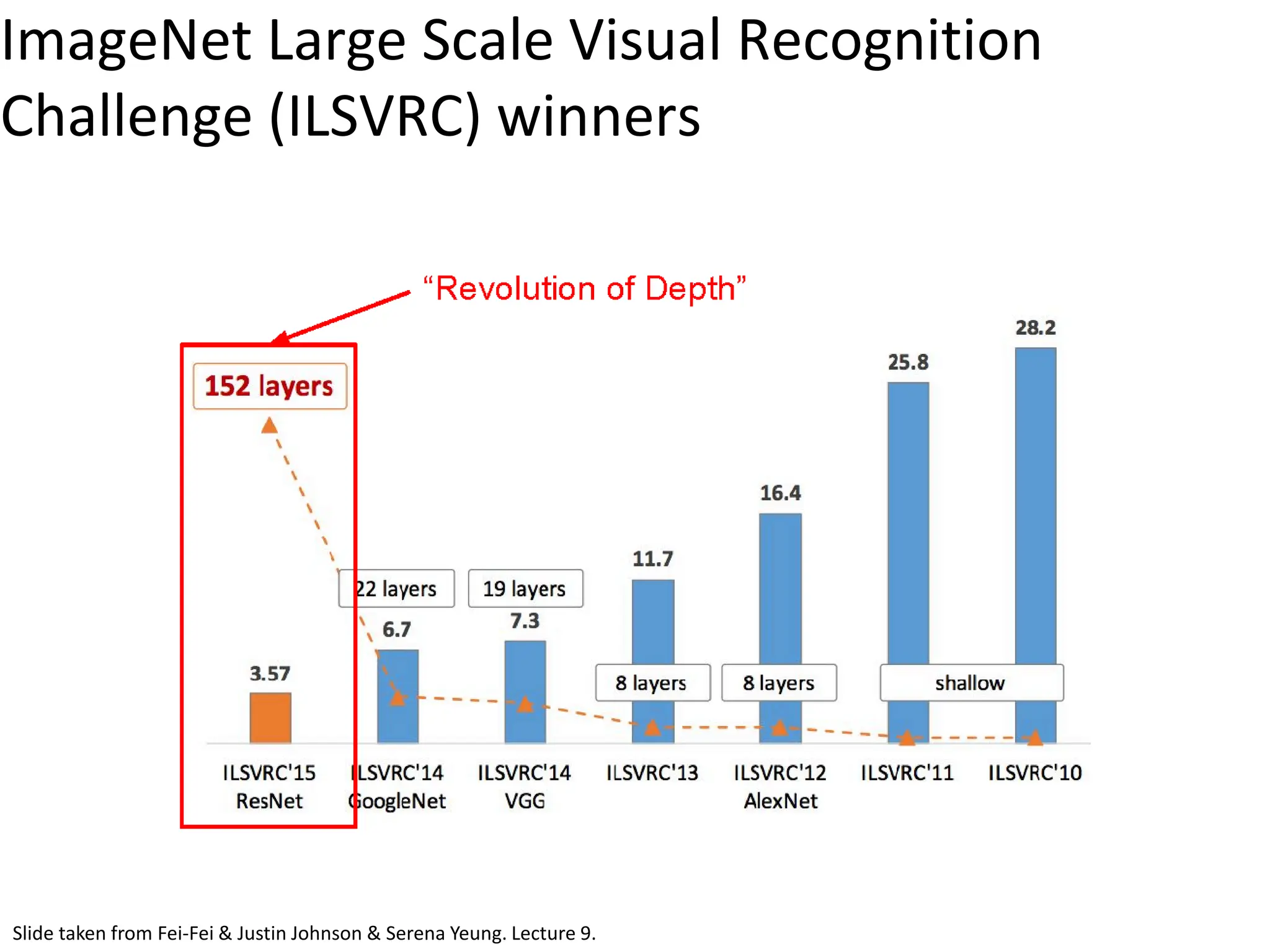
![ResNet • ILSVRC’15 classification winner (3.57% top 5 error, humans generally hover around a 5- 10% error rate) Swept all classification and detection competitions in ILSVRC’15 and COCO’15! Slide taken from Fei-Fei & Justin Johnson & Serena Yeung. Lecture 9. [He et al., 2015]](https://image.slidesharecdn.com/l03cnnsmk2-231007032320-a43fab35/75/CNN-Algorithm-90-2048.jpg)
![ResNet • What happens when we continue stacking deeper layers on a convolutional neural network? • 56-layer model performs worse on both training and test error -> The deeper model performs worse (not caused by overfitting)! Slide taken from Fei-Fei & Justin Johnson & Serena Yeung. Lecture 9. [He et al., 2015]](https://image.slidesharecdn.com/l03cnnsmk2-231007032320-a43fab35/75/CNN-Algorithm-91-2048.jpg)
![ResNet • Hypothesis: The problem is an optimization problem. Very deep networks are harder to optimize. • Solution: Use network layers to fit residual mapping instead of directly trying to fit a desired underlying mapping. • We will use skip connections allowing us to take the activation from one layer and feed it into another layer, much deeper into the network. • Use layers to fit residual F(x) = H(x) – x instead of H(x) directly Slide taken from Fei-Fei & Justin Johnson & Serena Yeung. Lecture 9. [He et al., 2015]](https://image.slidesharecdn.com/l03cnnsmk2-231007032320-a43fab35/75/CNN-Algorithm-92-2048.jpg)
![ResNet Residual Block Input x goes through conv-relu-conv series and gives us F(x). That result is then added to the original input x. Let’s call that H(x) = F(x) + x. In traditional CNNs, H(x) would just be equal to F(x). So, instead of just computing that transformation (straight from x to F(x)), we’re computing the term that we have to add, F(x), to the input, x. [He et al., 2015]](https://image.slidesharecdn.com/l03cnnsmk2-231007032320-a43fab35/75/CNN-Algorithm-93-2048.jpg)
![ResNet Short cut/ skip connection 𝑎𝑎[𝑙𝑙] 𝑎𝑎[𝑙𝑙+2] 𝐳𝐳[𝐥𝐥+𝟏𝟏] = 𝐖𝐖[𝐥𝐥+𝟏𝟏] 𝐚𝐚[𝐥𝐥] + 𝐛𝐛[𝐥𝐥+𝟏𝟏] 𝐚𝐚[𝐥𝐥+𝟏𝟏] = 𝐠𝐠(𝐳𝐳[𝐥𝐥+𝟏𝟏]) 𝐳𝐳[𝐥𝐥+𝟐𝟐] = 𝐖𝐖[𝐥𝐥+𝟐𝟐]𝐚𝐚[𝐥𝐥+𝟏𝟏] + 𝐛𝐛[𝐥𝐥+𝟐𝟐] 𝐚𝐚[𝐥𝐥+𝟐𝟐] = 𝐠𝐠(𝐳𝐳[𝐥𝐥+𝟐𝟐]) 𝑎𝑎[𝑙𝑙+1] a[l] a[l+1] 𝐋𝐋𝐋𝐋𝐋𝐋𝐋𝐋𝐋𝐋𝐋𝐋 𝐑𝐑𝐑𝐑𝐑𝐑𝐑𝐑 𝐋𝐋𝐋𝐋𝐋𝐋𝐋𝐋𝐋𝐋𝐋𝐋 𝐑𝐑𝐑𝐑𝐑𝐑𝐑𝐑 a[l+2] 𝐚𝐚[𝐥𝐥+𝟐𝟐] = 𝐠𝐠 𝐳𝐳 𝐥𝐥+𝟐𝟐 + 𝐚𝐚 𝐥𝐥 = 𝐠𝐠(𝐖𝐖[𝐥𝐥+𝟐𝟐] 𝐚𝐚[𝐥𝐥+𝟏𝟏] + 𝐛𝐛[𝐥𝐥+𝟐𝟐] + 𝐚𝐚 𝐥𝐥 ) [He et al., 2015]](https://image.slidesharecdn.com/l03cnnsmk2-231007032320-a43fab35/75/CNN-Algorithm-94-2048.jpg)
![ResNet Full ResNet architecture: • Stack residual blocks • Every residual block has two 3x3 conv layers • Periodically, double # of filters and downsample spatially using stride 2 (in each dimension) • Additional conv layer at the beginning • No FC layers at the end (only FC 1000 to output classes) [He et al., 2015] Slide taken from Fei-Fei & Justin Johnson & Serena Yeung. Lecture 9.](https://image.slidesharecdn.com/l03cnnsmk2-231007032320-a43fab35/75/CNN-Algorithm-95-2048.jpg)
![ResNet • Total depths of 34, 50, 101, or 152 layers for ImageNet • For deeper networks (ResNet-50+), use “bottleneck” layer to improve efficiency (similar to GoogLeNet) [He et al., 2015] Slide taken from Fei-Fei & Justin Johnson & Serena Yeung. Lecture 9.](https://image.slidesharecdn.com/l03cnnsmk2-231007032320-a43fab35/75/CNN-Algorithm-96-2048.jpg)
![ResNet Experimental Results: • Able to train very deep networks without degrading • Deeper networks now achieve lower training errors as expected [He et al., 2015] Slide taken from Fei-Fei & Justin Johnson & Serena Yeung. Lecture 9.](https://image.slidesharecdn.com/l03cnnsmk2-231007032320-a43fab35/75/CNN-Algorithm-97-2048.jpg)
![ResNet The best CNN architecture that we currently have and is a great innovation for the idea of residual learning. Even better than human performance! [He et al., 2015]](https://image.slidesharecdn.com/l03cnnsmk2-231007032320-a43fab35/75/CNN-Algorithm-98-2048.jpg)
![DeepBind [Alipanahi et al., 2015]](https://image.slidesharecdn.com/l03cnnsmk2-231007032320-a43fab35/75/CNN-Algorithm-116-2048.jpg)
![Predicting disease mutations [Alipanahi et al., 2015]](https://image.slidesharecdn.com/l03cnnsmk2-231007032320-a43fab35/75/CNN-Algorithm-117-2048.jpg)