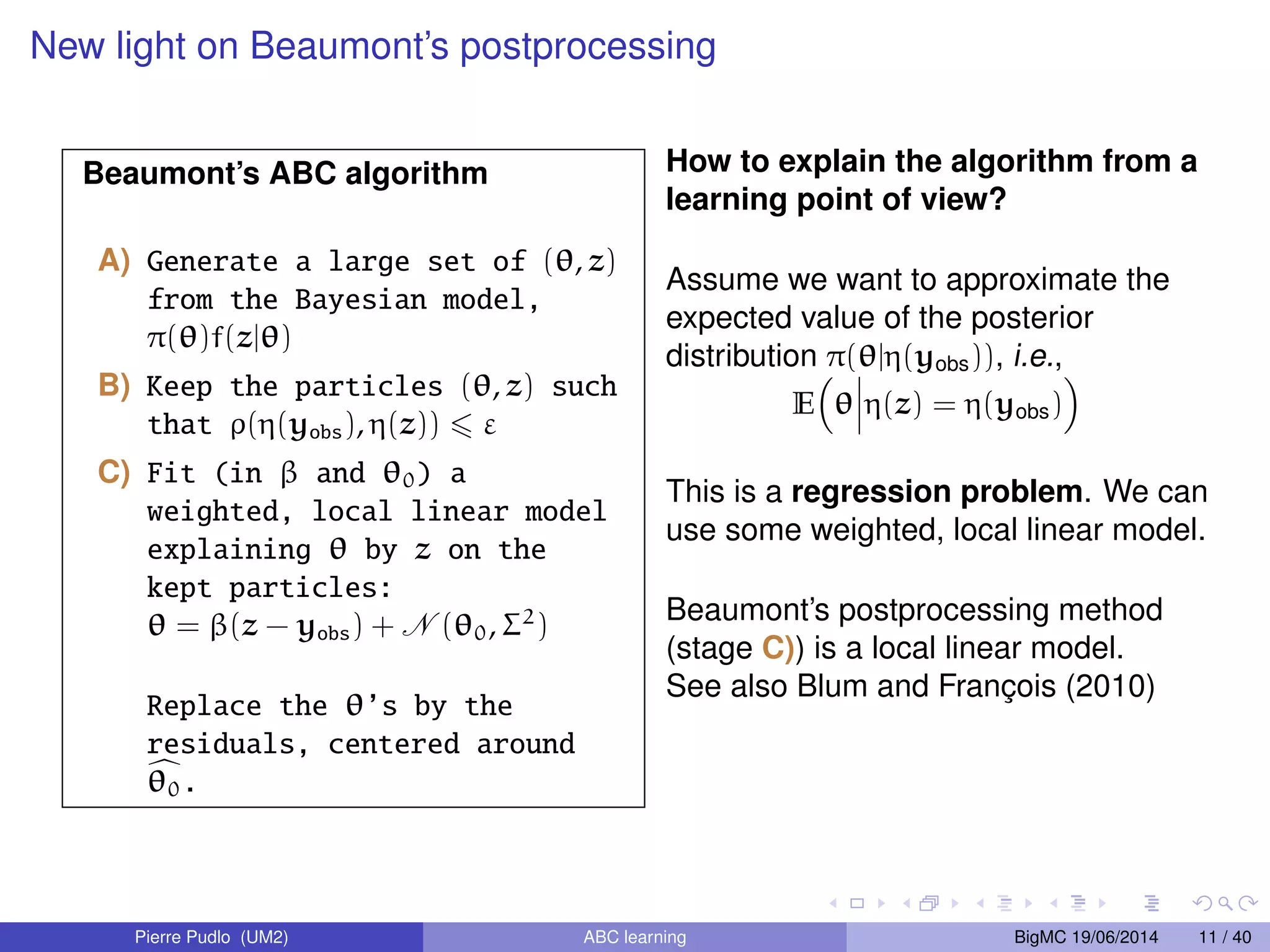
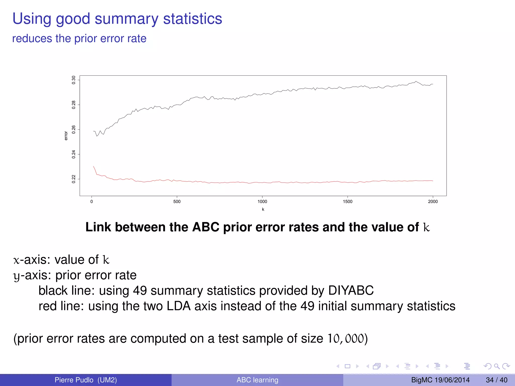
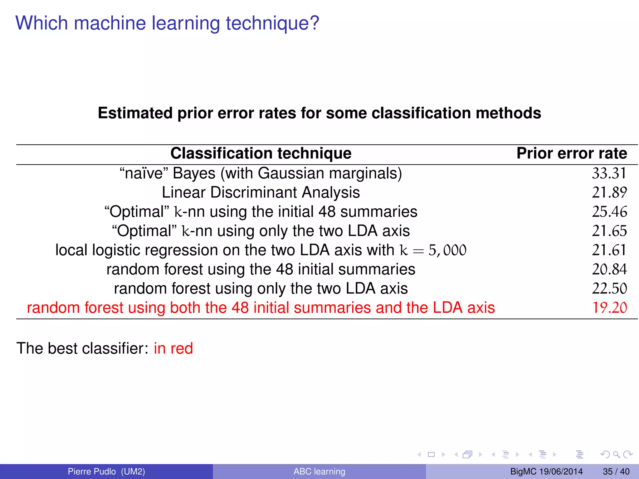
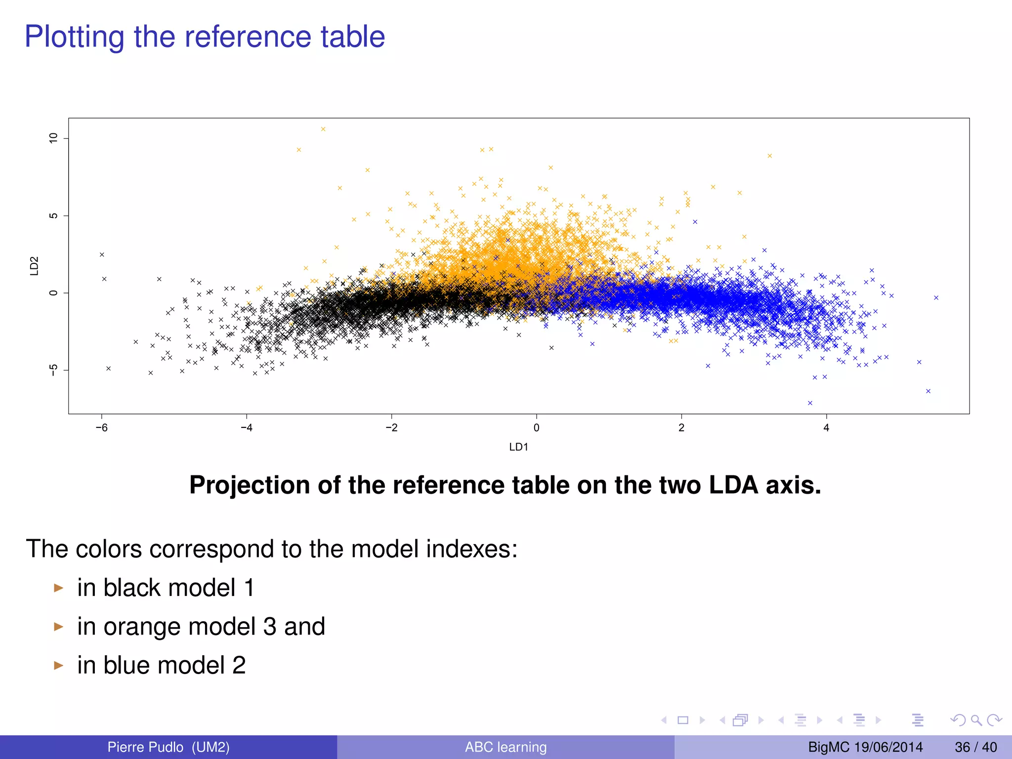
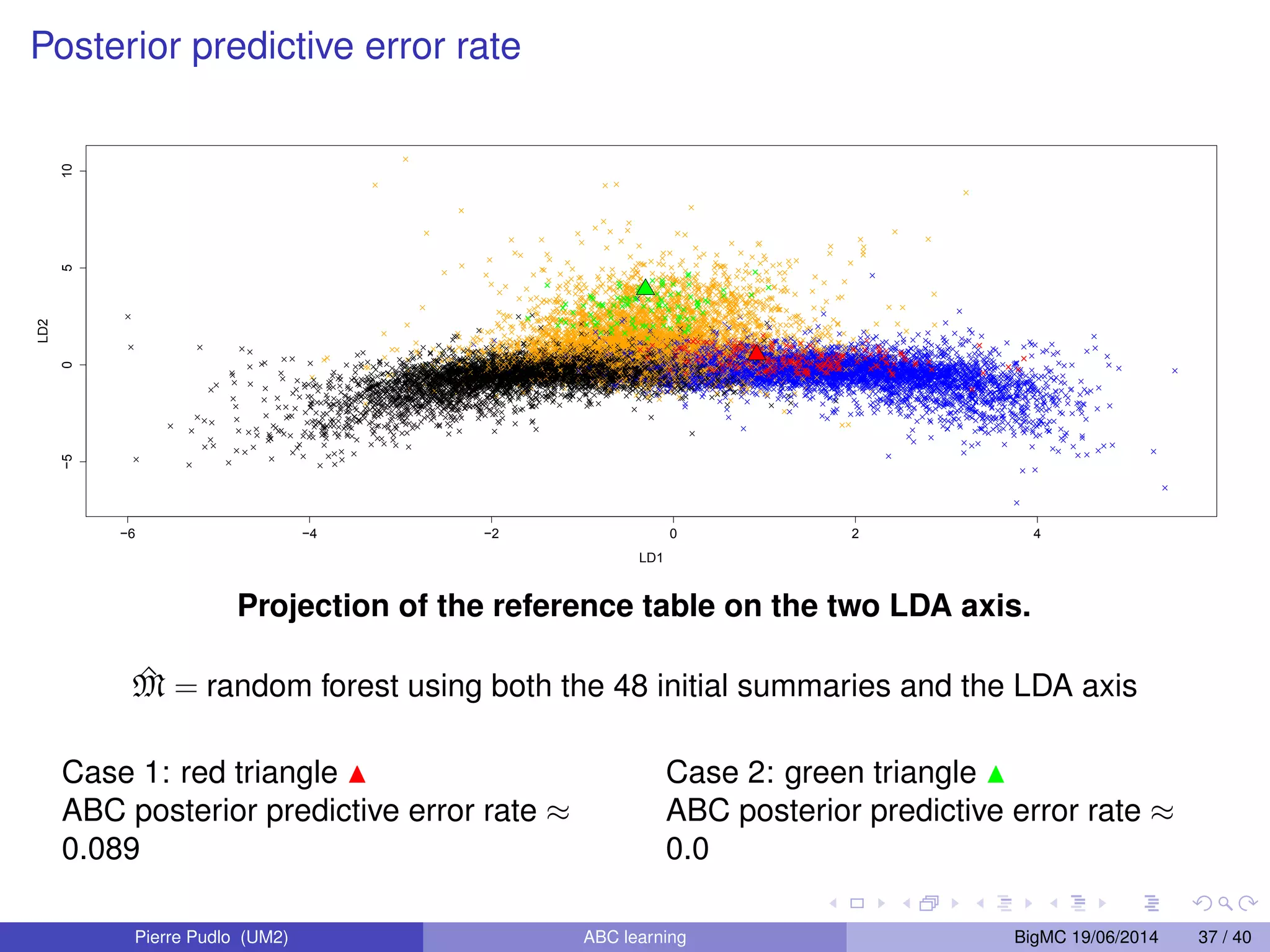
Download as PDF, PPTX
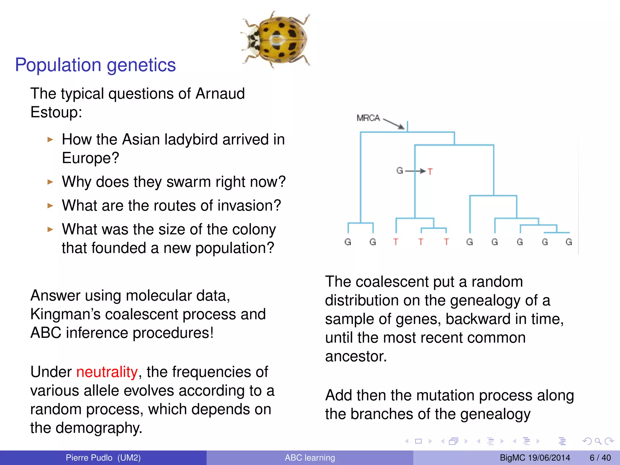
![Population genetics (cont’) Divergence Pop1 Pop1 Pop2 (a) t0 t Admixture r 1 - r 2.5 Conclusion 37 Pop1 Pop3 Pop2 (b) t0 t Migration m21 m12 Pop1 Pop2 (c) t0 t FIGURE 2.3: Représentations graphiques des trois types d’évènements inter-populationnels d’un scénario démographique. Il existe deux familles d’évènements inter-populationnels. La première famille est simple, elle correspond aux évènement inter-populationnels instantanés. C’est le cas d’une divergence ou d’une admixture. (a) Deux populations qui évoluent pour se fusionner dans le cas d’une divergence. (b) Trois po-pulations Between populations: three types of events, backward in time I the divergence is the fusion between two populations, I the admixture is the split of a population into two parts, I the migration allows the move of some lineages of a population to another. The goal is to discriminate between different population scenarios from a dataset of polymorphism (DNA sample) yobs observed at the present time. qui évoluent en parallèle pour une admixture. Pour cette t5 situation, chacun des tubes représente (on peut imaginer qu’il porte à l’intérieur) la généalogie de la population qui évolue indépendamment des autres suivant un coalescent de Kingman. La deuxième correspond à la présence d’une migration.(c) Cette situation est légèrement plus compliquée que la précédente à cause des flux de gènes (plus d’indépendance). Ici, un seul processus évolutif gouverne les deux populations réunies. La présence de migrations entre les populations Pop1 et Pop2 implique des déplacements de lignées d’une population à l’autre et ainsi la concurrence entre les évènements de coales-cence et de migration. A complex scenario: Ne04 Divergence Pop1 Ne1 Pop4 Ne4 Ne6 Pop6 s 1 - s Admixture Ne3 Pop3 Ne2 Pop2 Ne5 Pop5 Migration m0 m t04 t4 t = 0 Ne4 t3 t2 t1 r 1 - r FIGURE 2.1: Exemple d’un scénario évolutif complexe composé d’évènements inter-populationnels. Ce scénario implique quatre populations échantillonnées Pop1, . . . , Pop4 et deux autres populations non-observées Pop5 et Pop6. Les branches de ce schéma sont des tubes et le scénario démographique contraint la généalogie à rester à l’intérieur de ces tubes. La migration entre les populations Pop3 et Pop4 sur la période [0, t3] est paramétrée par les taux de migration m et m0. Les deux évènements d’admixture sont pa-ramétrés Pierre Pudlo (UM2) ABC learning BigMC 19/06/2014 7 / 40 par les dates t1 et t3 ainsi que les taux d’admixture respectifs r et s. Les trois évènements restants sont des divergences, respectivement en t2, t4 et t5. L’événement en t04 correspond à un changement de taille](https://image.slidesharecdn.com/bigmc2014-141021003808-conversion-gate01/75/Approximate-Bayesian-computation-and-machine-learning-BigMC-2014-7-2048.jpg)
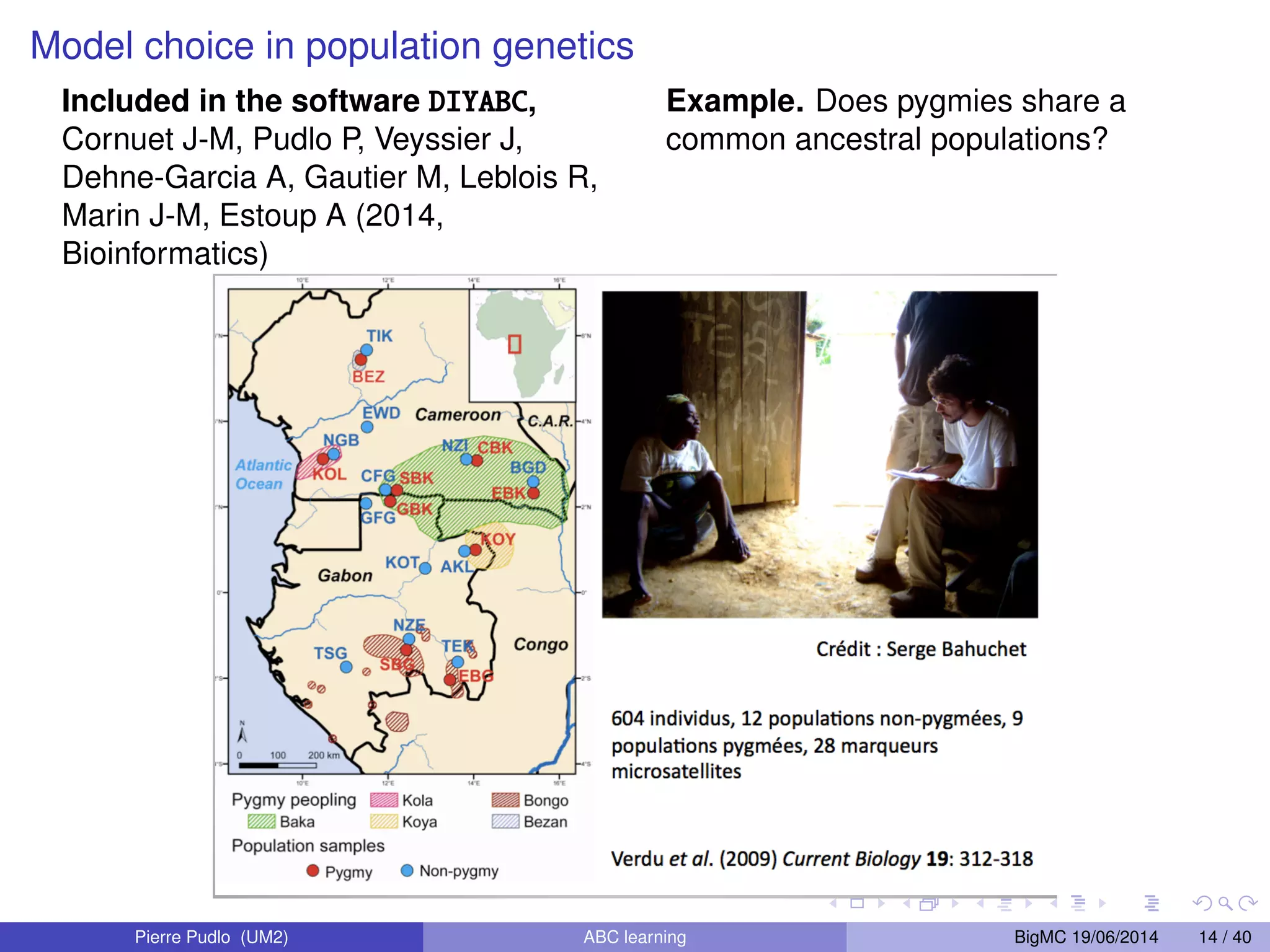
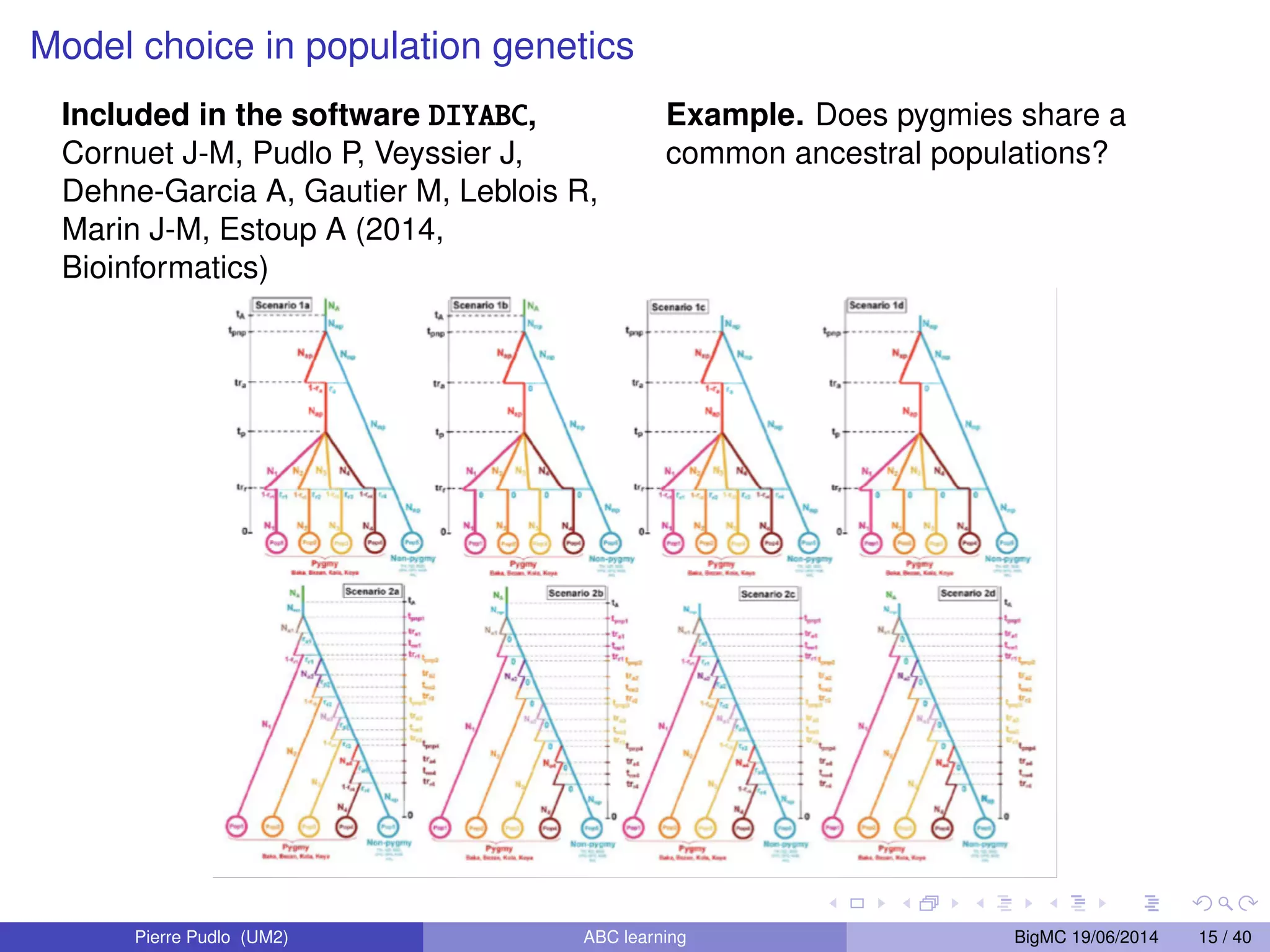
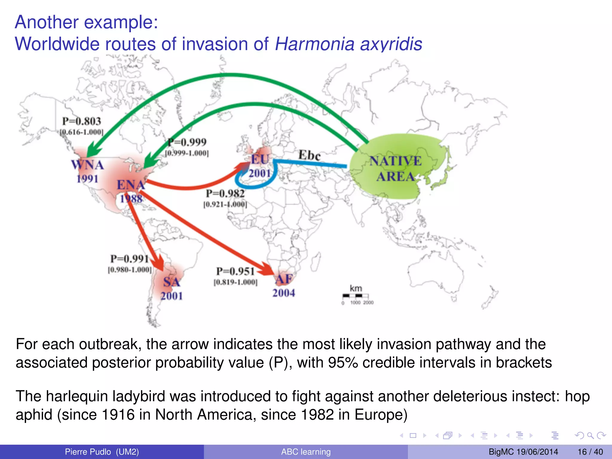
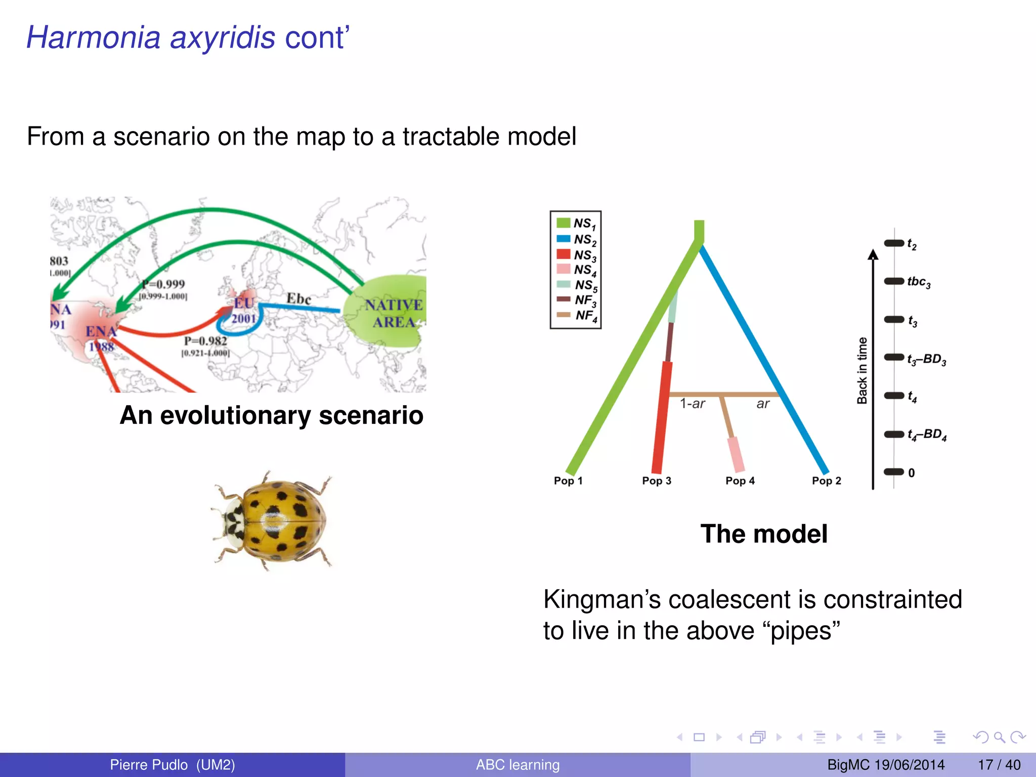
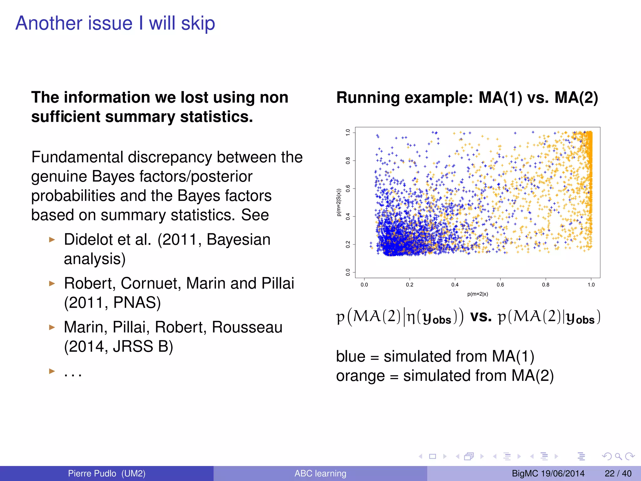

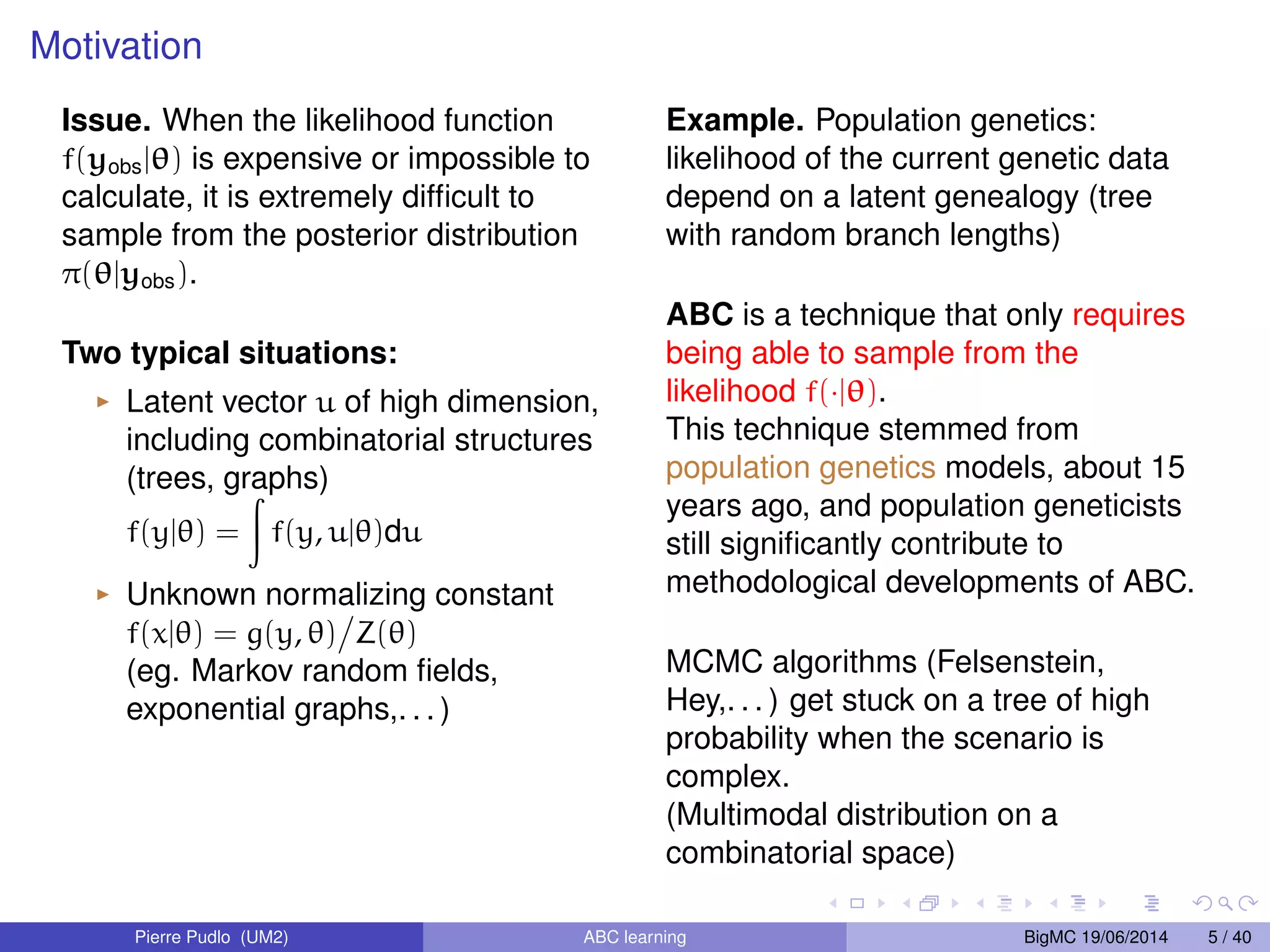
The document discusses Approximate Bayesian Computation (ABC), particularly in the context of population genetics, where it is used to infer demographic models from genetic data without needing to calculate likelihood functions. It details the methodology of ABC, including model choice and the use of genetic data for understanding population scenarios. The document highlights various examples of applications, including the study of the Asian ladybird's invasion routes and methods to analyze demographic models through ABC techniques.