Downloaded 33 times
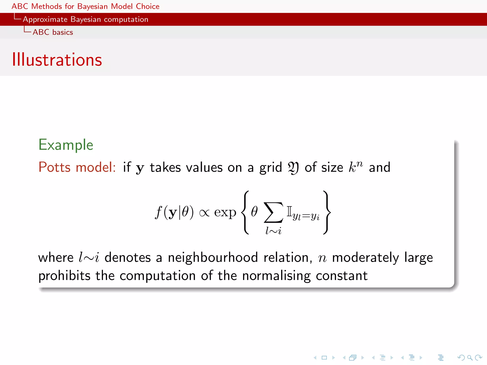
![ABC Methods for Bayesian Model Choice Approximate Bayesian computation ABC basics Illustrations Example Inference on CMB: in cosmology, study of the Cosmic Microwave Background via likelihoods immensely slow to computate (e.g WMAP, Plank), because of numerically costly spectral transforms [Data is a Fortran program] [Kilbinger et al., 2010, MNRAS]](https://image.slidesharecdn.com/zurich-110201155327-phpapp02/75/Workshop-on-Bayesian-Inference-for-Latent-Gaussian-Models-with-Applications-6-2048.jpg)
![ABC Methods for Bayesian Model Choice Approximate Bayesian computation ABC basics Illustrations Example Coalescence tree: in population genetics, reconstitution of a common ancestor from a sample of genes via a phylogenetic tree that is close to impossible to integrate out [100 processor days with 4 parameters] [Cornuet et al., 2009, Bioinformatics]](https://image.slidesharecdn.com/zurich-110201155327-phpapp02/75/Workshop-on-Bayesian-Inference-for-Latent-Gaussian-Models-with-Applications-7-2048.jpg)
![ABC Methods for Bayesian Model Choice Approximate Bayesian computation ABC basics The ABC method Bayesian setting: target is π(θ)f (x|θ) When likelihood f (x|θ) not in closed form, likelihood-free rejection technique: ABC algorithm For an observation y ∼ f (y|θ), under the prior π(θ), keep jointly simulating θ ∼ π(θ) , z ∼ f (z|θ ) , until the auxiliary variable z is equal to the observed value, z = y. [Tavar´ et al., 1997] e](https://image.slidesharecdn.com/zurich-110201155327-phpapp02/75/Workshop-on-Bayesian-Inference-for-Latent-Gaussian-Models-with-Applications-10-2048.jpg)
![ABC Methods for Bayesian Model Choice Approximate Bayesian computation ABC basics Why does it work?! The proof is trivial: f (θi ) ∝ π(θi )f (z|θi )Iy (z) z∈D ∝ π(θi )f (y|θi ) = π(θi |y) . [Accept–Reject 101]](https://image.slidesharecdn.com/zurich-110201155327-phpapp02/75/Workshop-on-Bayesian-Inference-for-Latent-Gaussian-Models-with-Applications-11-2048.jpg)
![ABC Methods for Bayesian Model Choice Approximate Bayesian computation ABC basics Earlier occurrence ‘Bayesian statistics and Monte Carlo methods are ideally suited to the task of passing many models over one dataset’ [Don Rubin, Annals of Statistics, 1984] Note Rubin (1984) does not promote this algorithm for likelihood-free simulation but frequentist intuition on posterior distributions: parameters from posteriors are more likely to be those that could have generated the data.](https://image.slidesharecdn.com/zurich-110201155327-phpapp02/75/Workshop-on-Bayesian-Inference-for-Latent-Gaussian-Models-with-Applications-12-2048.jpg)

![ABC Methods for Bayesian Model Choice Approximate Bayesian computation ABC basics ABC advances Simulating from the prior is often poor in efficiency Either modify the proposal distribution on θ to increase the density of x’s within the vicinity of y... [Marjoram et al, 2003; Bortot et al., 2007, Sisson et al., 2007]](https://image.slidesharecdn.com/zurich-110201155327-phpapp02/75/Workshop-on-Bayesian-Inference-for-Latent-Gaussian-Models-with-Applications-25-2048.jpg)
![ABC Methods for Bayesian Model Choice Approximate Bayesian computation ABC basics ABC advances Simulating from the prior is often poor in efficiency Either modify the proposal distribution on θ to increase the density of x’s within the vicinity of y... [Marjoram et al, 2003; Bortot et al., 2007, Sisson et al., 2007] ...or by viewing the problem as a conditional density estimation and by developing techniques to allow for larger [Beaumont et al., 2002]](https://image.slidesharecdn.com/zurich-110201155327-phpapp02/75/Workshop-on-Bayesian-Inference-for-Latent-Gaussian-Models-with-Applications-26-2048.jpg)
![ABC Methods for Bayesian Model Choice Approximate Bayesian computation ABC basics ABC advances Simulating from the prior is often poor in efficiency Either modify the proposal distribution on θ to increase the density of x’s within the vicinity of y... [Marjoram et al, 2003; Bortot et al., 2007, Sisson et al., 2007] ...or by viewing the problem as a conditional density estimation and by developing techniques to allow for larger [Beaumont et al., 2002] .....or even by including in the inferential framework [ABCµ ] [Ratmann et al., 2009]](https://image.slidesharecdn.com/zurich-110201155327-phpapp02/75/Workshop-on-Bayesian-Inference-for-Latent-Gaussian-Models-with-Applications-27-2048.jpg)
![ABC Methods for Bayesian Model Choice Approximate Bayesian computation Alphabet soup ABC-NP Better usage of [prior] simulations by adjustement: instead of throwing away θ such that ρ(η(z), η(y)) > , replace θs with locally regressed θ∗ = θ − {η(z) − η(y)}T β ˆ [Csill´ry et al., TEE, 2010] e ˆ where β is obtained by [NP] weighted least square regression on (η(z) − η(y)) with weights Kδ {ρ(η(z), η(y))} [Beaumont et al., 2002, Genetics]](https://image.slidesharecdn.com/zurich-110201155327-phpapp02/75/Workshop-on-Bayesian-Inference-for-Latent-Gaussian-Models-with-Applications-28-2048.jpg)
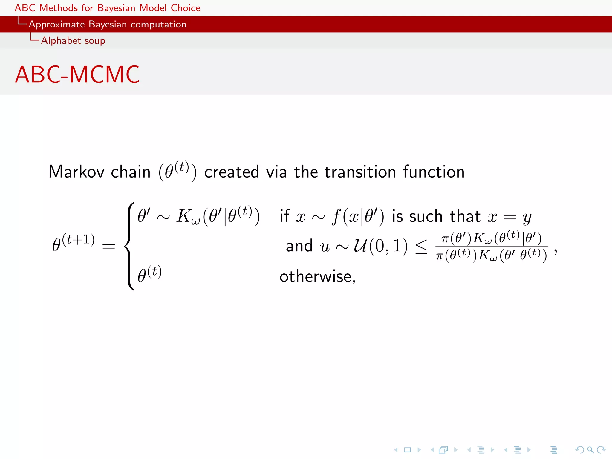
![ABC Methods for Bayesian Model Choice Approximate Bayesian computation Alphabet soup ABC-MCMC Markov chain (θ(t) ) created via the transition function θ ∼ Kω (θ |θ(t) ) if x ∼ f (x|θ ) is such that x = y π(θ )Kω (t) |θ ) θ (t+1) = and u ∼ U(0, 1) ≤ π(θ(t) )K (θ |θ(t) ) , ω (θ (t) θ otherwise, has the posterior π(θ|y) as stationary distribution [Marjoram et al, 2003]](https://image.slidesharecdn.com/zurich-110201155327-phpapp02/75/Workshop-on-Bayesian-Inference-for-Latent-Gaussian-Models-with-Applications-30-2048.jpg)
![ABC Methods for Bayesian Model Choice Approximate Bayesian computation Alphabet soup ABC-MCMC (2) Algorithm 2 Likelihood-free MCMC sampler Use Algorithm 1 to get (θ(0) , z(0) ) for t = 1 to N do Generate θ from Kω ·|θ(t−1) , Generate z from the likelihood f (·|θ ), Generate u from U[0,1] , π(θ )Kω (θ(t−1) |θ ) if u ≤ I π(θ(t−1) Kω (θ |θ(t−1) ) A ,y (z ) then set (θ(t) , z(t) ) = (θ , z ) else (θ(t) , z(t) )) = (θ(t−1) , z(t−1) ), end if end for](https://image.slidesharecdn.com/zurich-110201155327-phpapp02/75/Workshop-on-Bayesian-Inference-for-Latent-Gaussian-Models-with-Applications-31-2048.jpg)
![ABC Methods for Bayesian Model Choice Approximate Bayesian computation Alphabet soup ABCµ [Ratmann, Andrieu, Wiuf and Richardson, 2009, PNAS] Use of a joint density f (θ, |y) ∝ ξ( |y, θ) × πθ (θ) × π ( ) where y is the data, and ξ( |y, θ) is the prior predictive density of ρ(η(z), η(y)) given θ and x when z ∼ f (z|θ)](https://image.slidesharecdn.com/zurich-110201155327-phpapp02/75/Workshop-on-Bayesian-Inference-for-Latent-Gaussian-Models-with-Applications-33-2048.jpg)
![ABC Methods for Bayesian Model Choice Approximate Bayesian computation Alphabet soup ABCµ [Ratmann, Andrieu, Wiuf and Richardson, 2009, PNAS] Use of a joint density f (θ, |y) ∝ ξ( |y, θ) × πθ (θ) × π ( ) where y is the data, and ξ( |y, θ) is the prior predictive density of ρ(η(z), η(y)) given θ and x when z ∼ f (z|θ) Warning! Replacement of ξ( |y, θ) with a non-parametric kernel approximation.](https://image.slidesharecdn.com/zurich-110201155327-phpapp02/75/Workshop-on-Bayesian-Inference-for-Latent-Gaussian-Models-with-Applications-34-2048.jpg)
![ABC Methods for Bayesian Model Choice Approximate Bayesian computation Alphabet soup ABCµ details Multidimensional distances ρk (k = 1, . . . , K) and errors k = ρk (ηk (z), ηk (y)), with ˆ 1 k ∼ ξk ( |y, θ) ≈ ξk ( |y, θ) = K[{ k −ρk (ηk (zb ), ηk (y))}/hk ] Bhk b ˆ then used in replacing ξ( |y, θ) with mink ξk ( |y, θ)](https://image.slidesharecdn.com/zurich-110201155327-phpapp02/75/Workshop-on-Bayesian-Inference-for-Latent-Gaussian-Models-with-Applications-35-2048.jpg)
![ABC Methods for Bayesian Model Choice Approximate Bayesian computation Alphabet soup ABCµ details Multidimensional distances ρk (k = 1, . . . , K) and errors k = ρk (ηk (z), ηk (y)), with ˆ 1 k ∼ ξk ( |y, θ) ≈ ξk ( |y, θ) = K[{ k −ρk (ηk (zb ), ηk (y))}/hk ] Bhk b ˆ then used in replacing ξ( |y, θ) with mink ξk ( |y, θ) ABCµ involves acceptance probability ˆ π(θ , ) q(θ , θ)q( , ) mink ξk ( |y, θ ) ˆ π(θ, ) q(θ, θ )q( , ) mink ξk ( |y, θ)](https://image.slidesharecdn.com/zurich-110201155327-phpapp02/75/Workshop-on-Bayesian-Inference-for-Latent-Gaussian-Models-with-Applications-36-2048.jpg)
![ABC Methods for Bayesian Model Choice Approximate Bayesian computation Alphabet soup ABCµ multiple errors [ c Ratmann et al., PNAS, 2009]](https://image.slidesharecdn.com/zurich-110201155327-phpapp02/75/Workshop-on-Bayesian-Inference-for-Latent-Gaussian-Models-with-Applications-37-2048.jpg)
![ABC Methods for Bayesian Model Choice Approximate Bayesian computation Alphabet soup ABCµ for model choice [ c Ratmann et al., PNAS, 2009]](https://image.slidesharecdn.com/zurich-110201155327-phpapp02/75/Workshop-on-Bayesian-Inference-for-Latent-Gaussian-Models-with-Applications-38-2048.jpg)
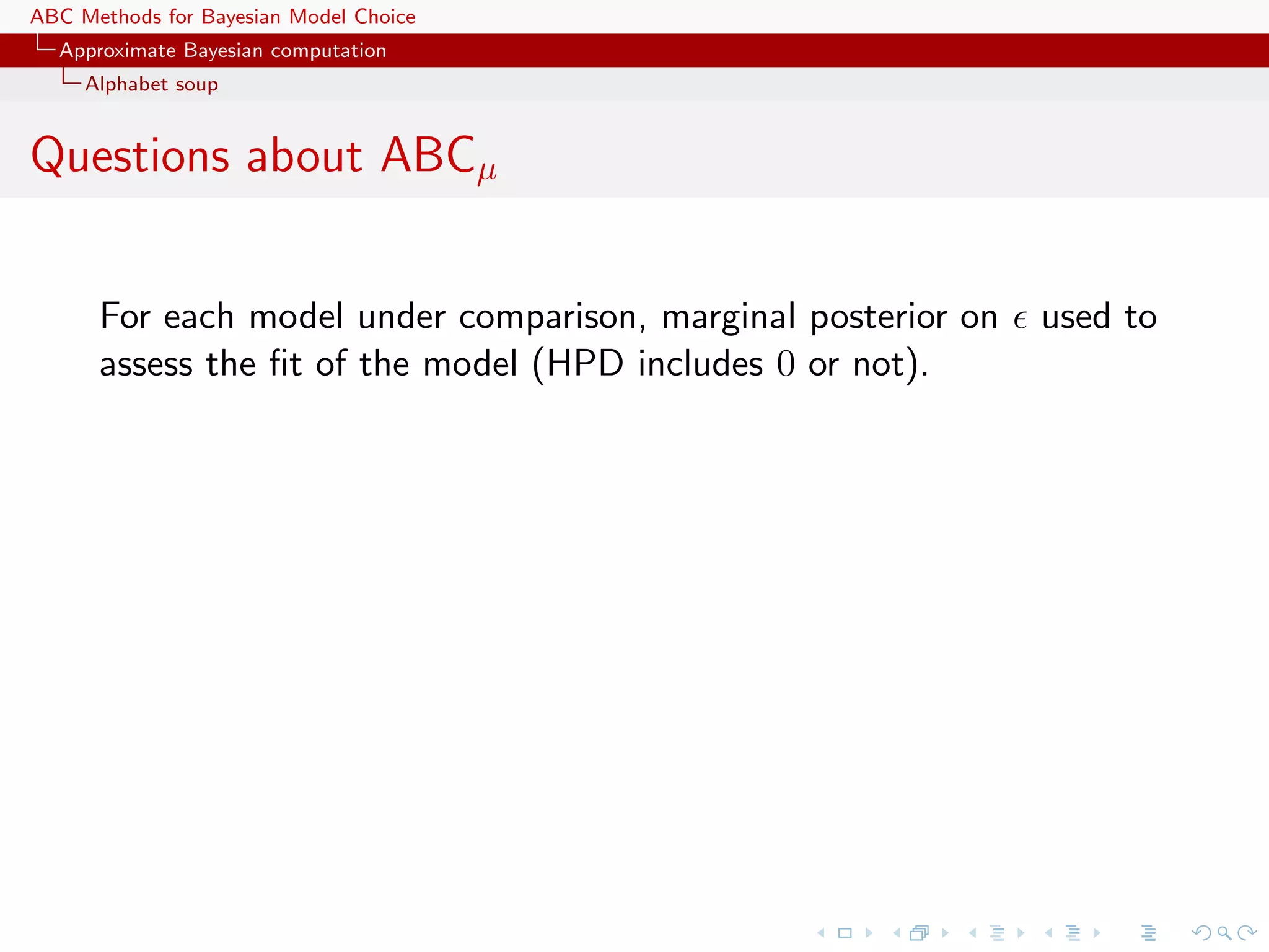
![ABC Methods for Bayesian Model Choice Approximate Bayesian computation Alphabet soup Questions about ABCµ For each model under comparison, marginal posterior on used to assess the fit of the model (HPD includes 0 or not). Is the data informative about ? [Identifiability] How is the prior π( ) impacting the comparison? How is using both ξ( |x0 , θ) and π ( ) compatible with a standard probability model? [remindful of Wilkinson] Where is the penalisation for complexity in the model comparison? [X, Mengersen & Chen, 2010, PNAS]](https://image.slidesharecdn.com/zurich-110201155327-phpapp02/75/Workshop-on-Bayesian-Inference-for-Latent-Gaussian-Models-with-Applications-40-2048.jpg)
![ABC Methods for Bayesian Model Choice Approximate Bayesian computation Alphabet soup A PMC version Use of the same kernel idea as ABC-PRC but with IS correction Generate a sample at iteration t by N (t) (t−1) (t−1) πt (θ ) ∝ ˆ ωj Kt (θ(t) |θj ) j=1 modulo acceptance of the associated xt , and use an importance (t) weight associated with an accepted simulation θi (t) (t) (t) ωi ∝ π(θi ) πt (θi ) . ˆ c Still likelihood free [Beaumont et al., Biometrika, 2009]](https://image.slidesharecdn.com/zurich-110201155327-phpapp02/75/Workshop-on-Bayesian-Inference-for-Latent-Gaussian-Models-with-Applications-41-2048.jpg)
![ABC Methods for Bayesian Model Choice Approximate Bayesian computation Alphabet soup Sequential Monte Carlo SMC is a simulation technique to approximate a sequence of related probability distributions πn with π0 “easy” and πT target. Iterated IS as PMC: particles moved from time n to time n via kernel Kn and use of a sequence of extended targets πn˜ n πn (z0:n ) = πn (zn ) ˜ Lj (zj+1 , zj ) j=0 where the Lj ’s are backward Markov kernels [check that πn (zn ) is a marginal] [Del Moral, Doucet & Jasra, Series B, 2006]](https://image.slidesharecdn.com/zurich-110201155327-phpapp02/75/Workshop-on-Bayesian-Inference-for-Latent-Gaussian-Models-with-Applications-42-2048.jpg)
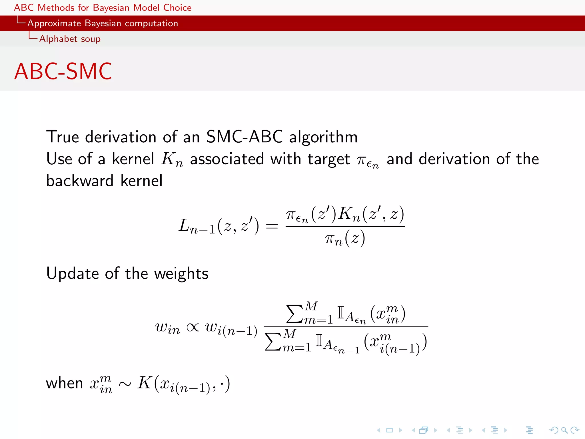
![ABC Methods for Bayesian Model Choice Approximate Bayesian computation Alphabet soup Properties of ABC-SMC The ABC-SMC method properly uses a backward kernel L(z, z ) to simplify the importance weight and to remove the dependence on the unknown likelihood from this weight. Update of importance weights is reduced to the ratio of the proportions of surviving particles Major assumption: the forward kernel K is supposed to be invariant against the true target [tempered version of the true posterior]](https://image.slidesharecdn.com/zurich-110201155327-phpapp02/75/Workshop-on-Bayesian-Inference-for-Latent-Gaussian-Models-with-Applications-44-2048.jpg)
![ABC Methods for Bayesian Model Choice Approximate Bayesian computation Alphabet soup Properties of ABC-SMC The ABC-SMC method properly uses a backward kernel L(z, z ) to simplify the importance weight and to remove the dependence on the unknown likelihood from this weight. Update of importance weights is reduced to the ratio of the proportions of surviving particles Major assumption: the forward kernel K is supposed to be invariant against the true target [tempered version of the true posterior] Adaptivity in ABC-SMC algorithm only found in on-line construction of the thresholds t , slowly enough to keep a large number of accepted transitions [Del Moral, Doucet & Jasra, 2009]](https://image.slidesharecdn.com/zurich-110201155327-phpapp02/75/Workshop-on-Bayesian-Inference-for-Latent-Gaussian-Models-with-Applications-45-2048.jpg)
![ABC Methods for Bayesian Model Choice Approximate Bayesian computation Calibration of ABC Which summary statistics? Fundamental difficulty of the choice of the summary statistic when there is no non-trivial sufficient statistic [except when done by the experimenters in the field]](https://image.slidesharecdn.com/zurich-110201155327-phpapp02/75/Workshop-on-Bayesian-Inference-for-Latent-Gaussian-Models-with-Applications-46-2048.jpg)
![ABC Methods for Bayesian Model Choice Approximate Bayesian computation Calibration of ABC Which summary statistics? Fundamental difficulty of the choice of the summary statistic when there is no non-trivial sufficient statistic [except when done by the experimenters in the field] Starting from a large collection of summary statistics is available, Joyce and Marjoram (2008) consider the sequential inclusion into the ABC target, with a stopping rule based on a likelihood ratio test.](https://image.slidesharecdn.com/zurich-110201155327-phpapp02/75/Workshop-on-Bayesian-Inference-for-Latent-Gaussian-Models-with-Applications-47-2048.jpg)
![ABC Methods for Bayesian Model Choice Approximate Bayesian computation Calibration of ABC Which summary statistics? Fundamental difficulty of the choice of the summary statistic when there is no non-trivial sufficient statistic [except when done by the experimenters in the field] Starting from a large collection of summary statistics is available, Joyce and Marjoram (2008) consider the sequential inclusion into the ABC target, with a stopping rule based on a likelihood ratio test. Does not taking into account the sequential nature of the tests Depends on parameterisation Order of inclusion matters.](https://image.slidesharecdn.com/zurich-110201155327-phpapp02/75/Workshop-on-Bayesian-Inference-for-Latent-Gaussian-Models-with-Applications-48-2048.jpg)
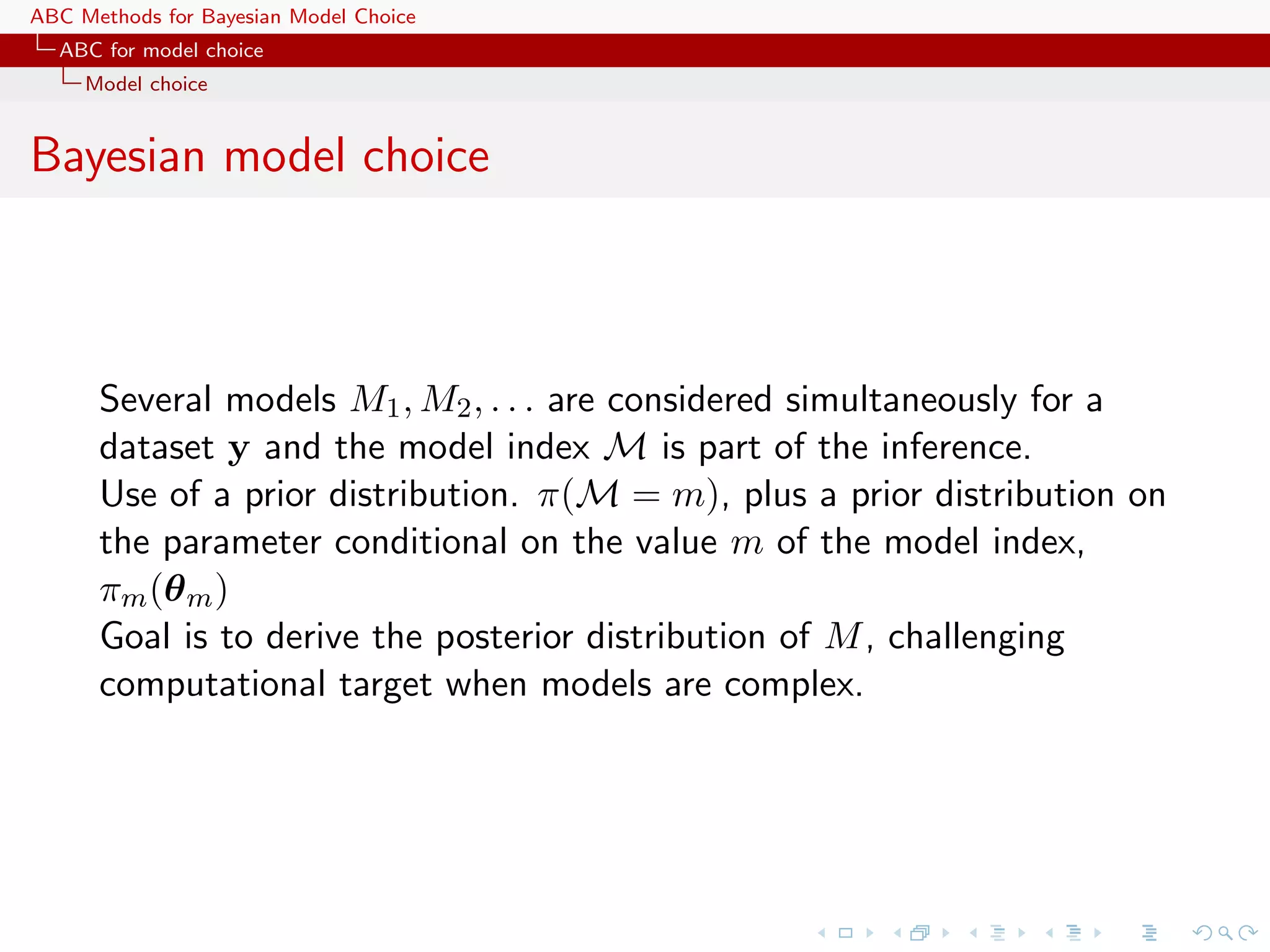
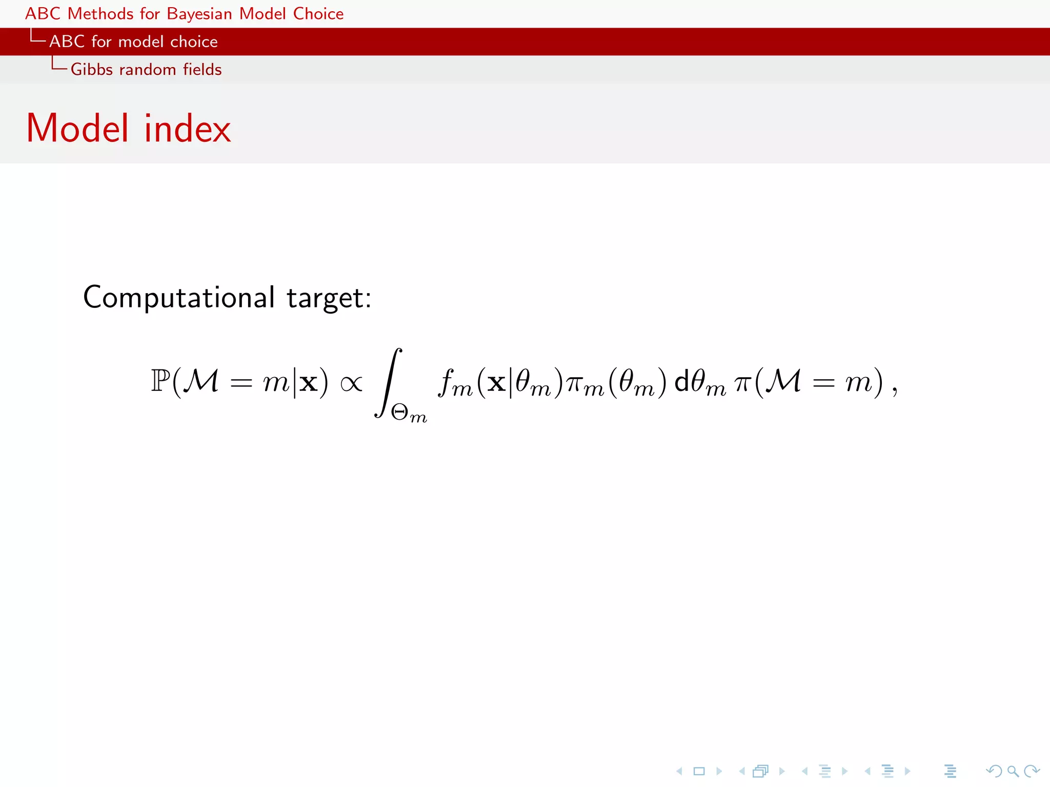
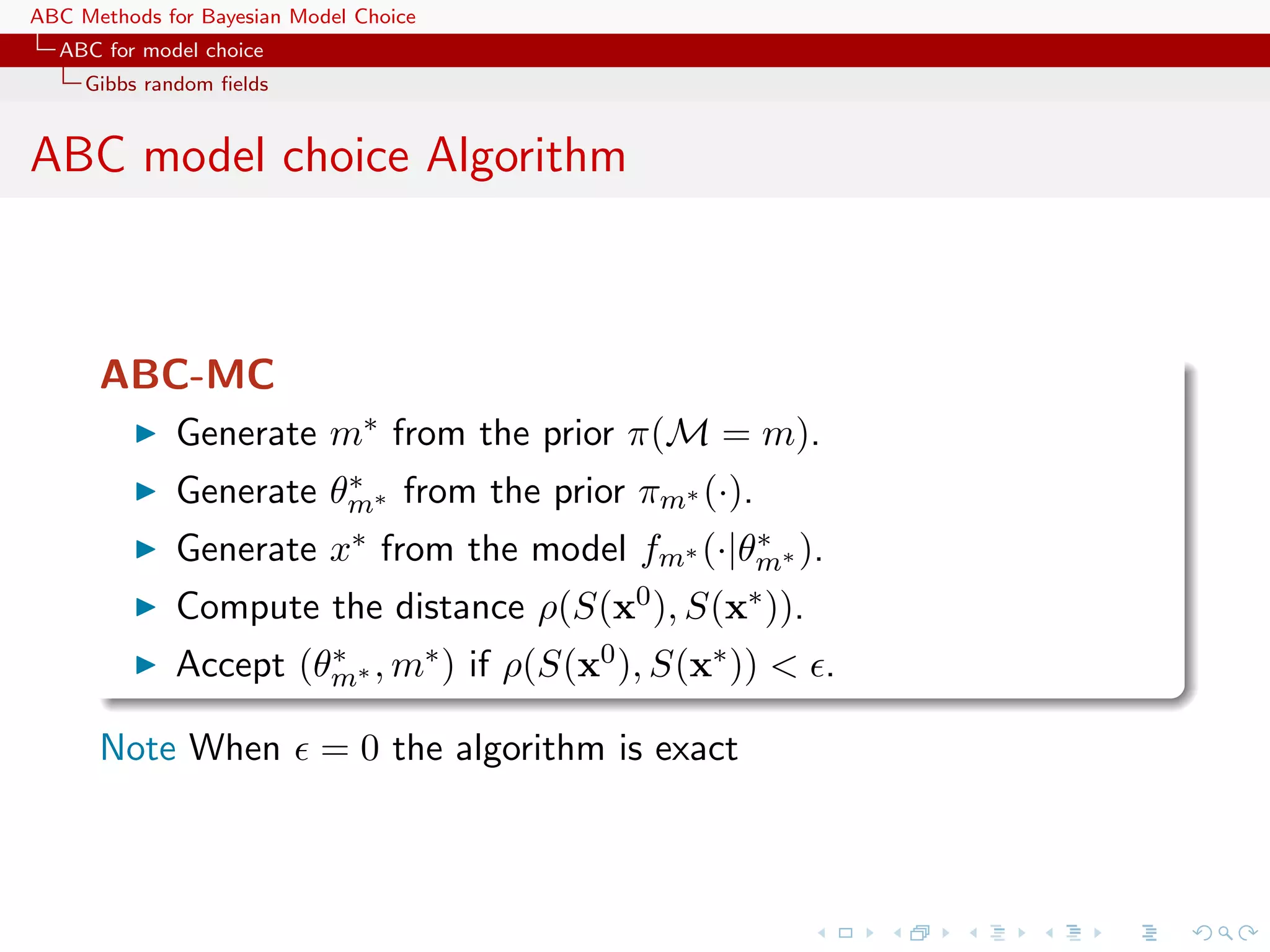
![ABC Methods for Bayesian Model Choice ABC for model choice Model choice Generic ABC for model choice Algorithm 3 Likelihood-free model choice sampler (ABC-MC) for t = 1 to T do repeat Generate m from the prior π(M = m) Generate θ m from the prior πm (θ m ) Generate z from the model fm (z|θ m ) until ρ{η(z), η(y)} < Set m(t) = m and θ (t) = θ m end for [Toni, Welch, Strelkowa, Ipsen & Stumpf, 2009]](https://image.slidesharecdn.com/zurich-110201155327-phpapp02/75/Workshop-on-Bayesian-Inference-for-Latent-Gaussian-Models-with-Applications-51-2048.jpg)
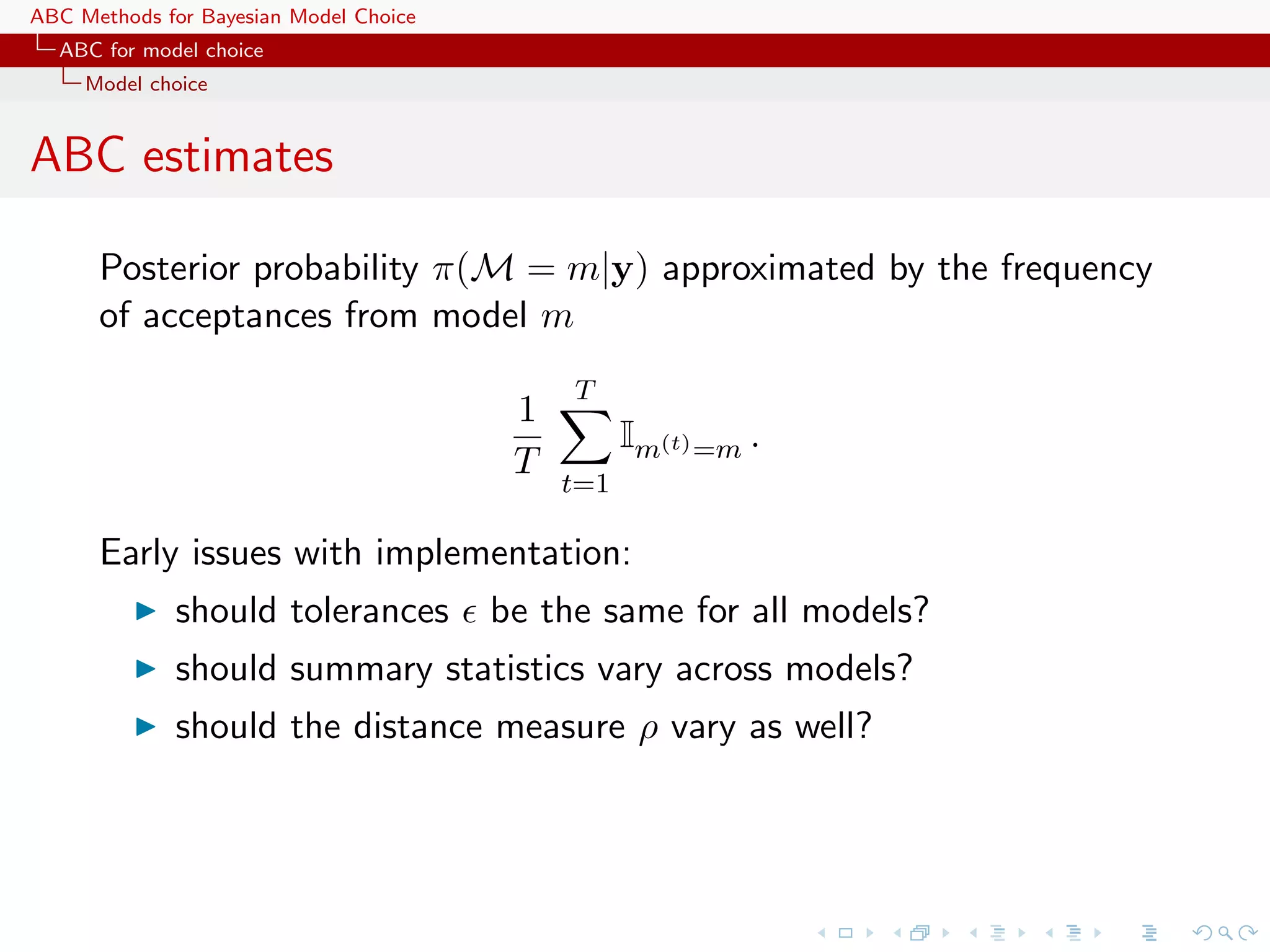
![ABC Methods for Bayesian Model Choice ABC for model choice Model choice ABC estimates Posterior probability π(M = m|y) approximated by the frequency of acceptances from model m T 1 Im(t) =m . T t=1 Early issues with implementation: should tolerances be the same for all models? should summary statistics vary across models? should the distance measure ρ vary as well? Extension to a weighted polychotomous logistic regression estimate of π(M = m|y), with non-parametric kernel weights [Cornuet et al., DIYABC, 2009]](https://image.slidesharecdn.com/zurich-110201155327-phpapp02/75/Workshop-on-Bayesian-Inference-for-Latent-Gaussian-Models-with-Applications-53-2048.jpg)
![ABC Methods for Bayesian Model Choice ABC for model choice Model choice The Great ABC controversy [# 1?] On-going controvery in phylogeographic genetics about the validity of using ABC for testing Against: Templeton, 2008, 2009, 2010a, 2010b, 2010c argues that nested hypotheses cannot have higher probabilities than nesting hypotheses (!)](https://image.slidesharecdn.com/zurich-110201155327-phpapp02/75/Workshop-on-Bayesian-Inference-for-Latent-Gaussian-Models-with-Applications-54-2048.jpg)
![ABC Methods for Bayesian Model Choice ABC for model choice Model choice The Great ABC controversy [# 1?] On-going controvery in phylogeographic genetics about the validity of using ABC for testing Replies: Fagundes et al., 2008, Against: Templeton, 2008, Beaumont et al., 2010, Berger et 2009, 2010a, 2010b, 2010c al., 2010, Csill`ry et al., 2010 e argues that nested hypotheses point out that the criticisms are cannot have higher probabilities addressed at [Bayesian] than nesting hypotheses (!) model-based inference and have nothing to do with ABC...](https://image.slidesharecdn.com/zurich-110201155327-phpapp02/75/Workshop-on-Bayesian-Inference-for-Latent-Gaussian-Models-with-Applications-55-2048.jpg)
![ABC Methods for Bayesian Model Choice ABC for model choice Generic ABC model choice Back to sufficiency ‘Sufficient statistics for individual models are unlikely to be very informative for the model probability. This is already well known and understood by the ABC-user community.’ [Scott Sisson, Jan. 31, 2011, ’Og]](https://image.slidesharecdn.com/zurich-110201155327-phpapp02/75/Workshop-on-Bayesian-Inference-for-Latent-Gaussian-Models-with-Applications-70-2048.jpg)
![ABC Methods for Bayesian Model Choice ABC for model choice Generic ABC model choice Back to sufficiency ‘Sufficient statistics for individual models are unlikely to be very informative for the model probability. This is already well known and understood by the ABC-user community.’ [Scott Sisson, Jan. 31, 2011, ’Og] If η1 (x) sufficient statistic for model m = 1 and parameter θ1 and η2 (x) sufficient statistic for model m = 2 and parameter θ2 , (η1 (x), η2 (x)) is not always sufficient for (m, θm )](https://image.slidesharecdn.com/zurich-110201155327-phpapp02/75/Workshop-on-Bayesian-Inference-for-Latent-Gaussian-Models-with-Applications-71-2048.jpg)
![ABC Methods for Bayesian Model Choice ABC for model choice Generic ABC model choice Back to sufficiency ‘Sufficient statistics for individual models are unlikely to be very informative for the model probability. This is already well known and understood by the ABC-user community.’ [Scott Sisson, Jan. 31, 2011, ’Og] If η1 (x) sufficient statistic for model m = 1 and parameter θ1 and η2 (x) sufficient statistic for model m = 2 and parameter θ2 , (η1 (x), η2 (x)) is not always sufficient for (m, θm ) c Potential loss of information at the testing level](https://image.slidesharecdn.com/zurich-110201155327-phpapp02/75/Workshop-on-Bayesian-Inference-for-Latent-Gaussian-Models-with-Applications-72-2048.jpg)
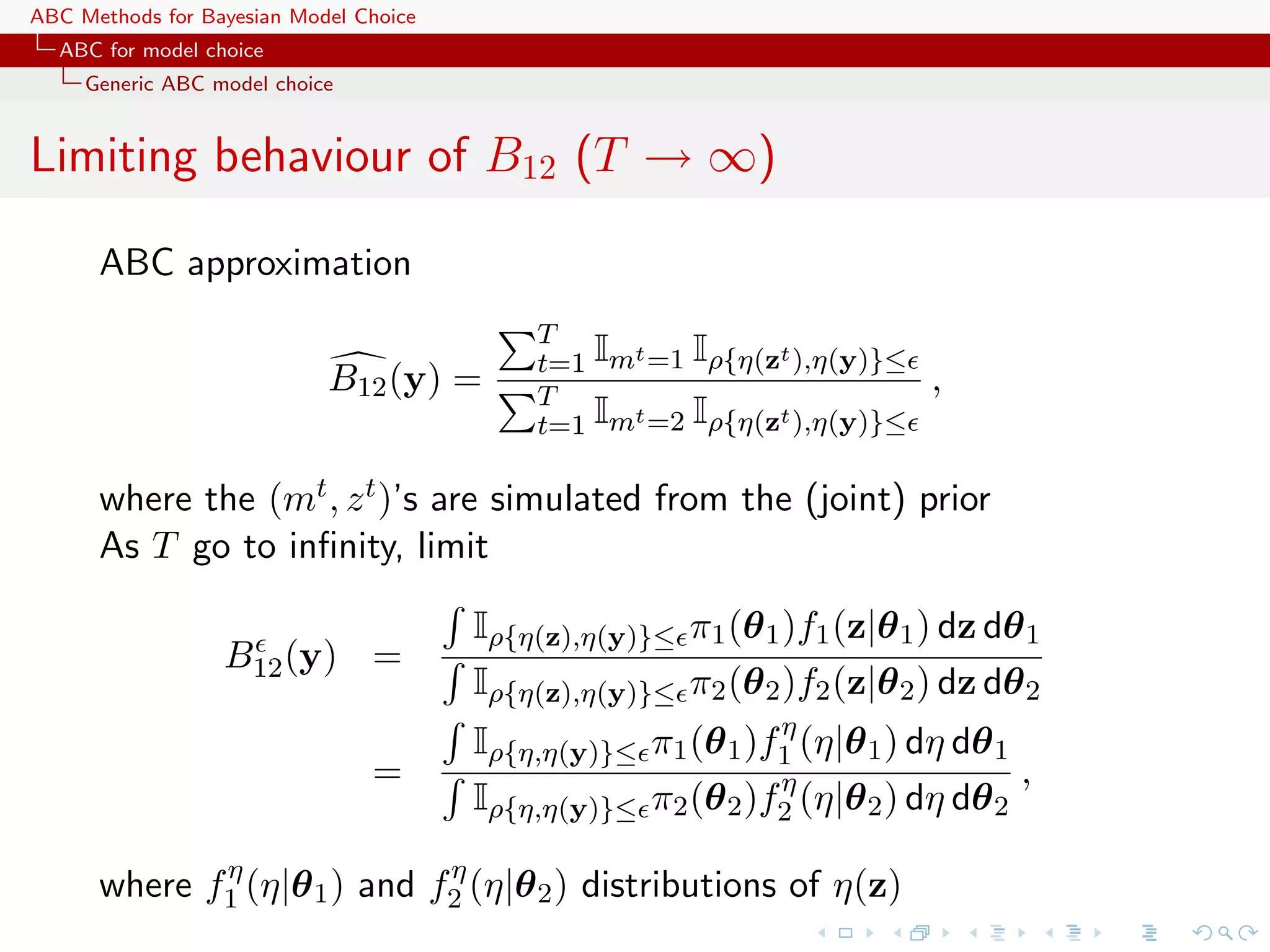
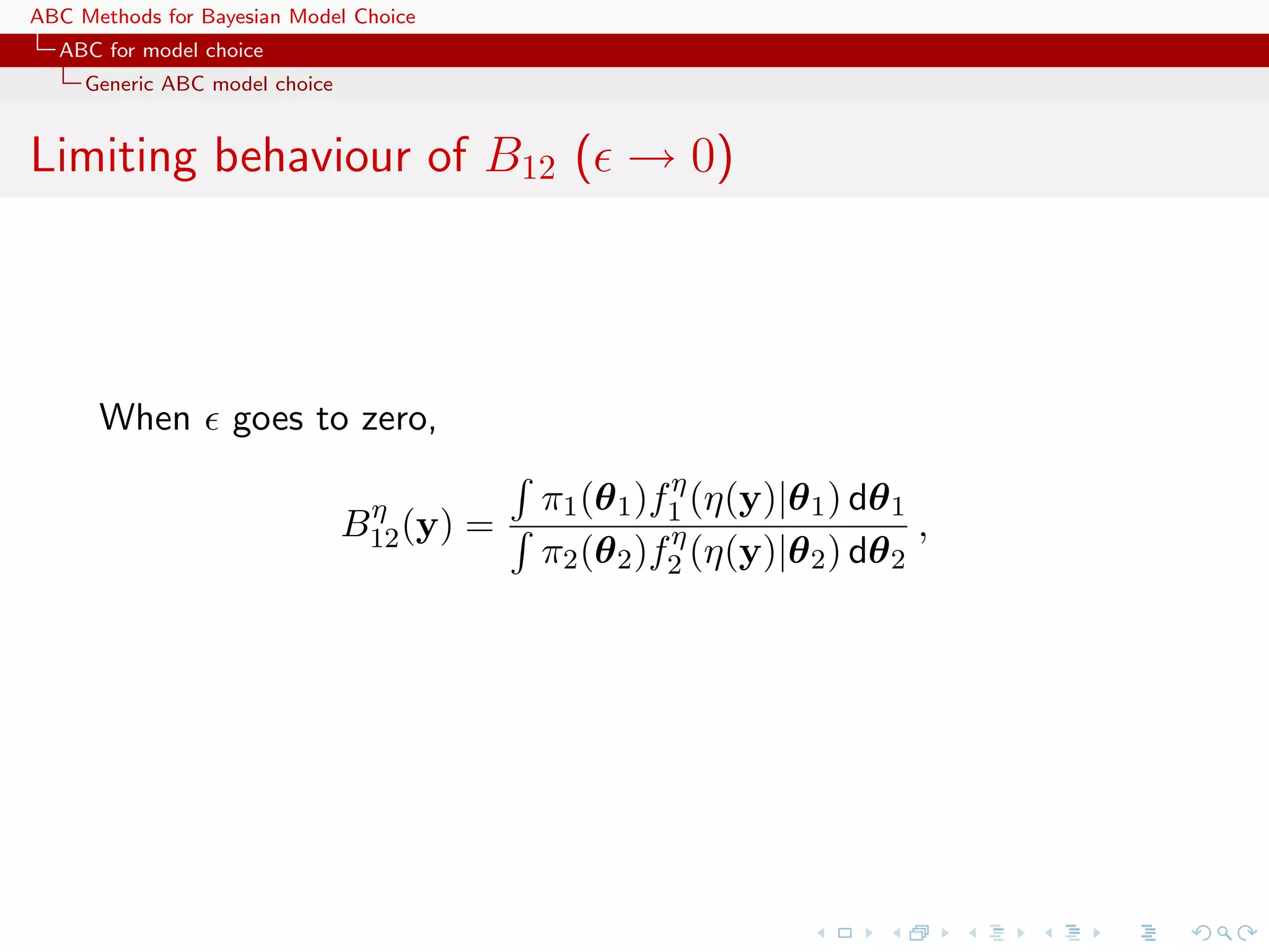
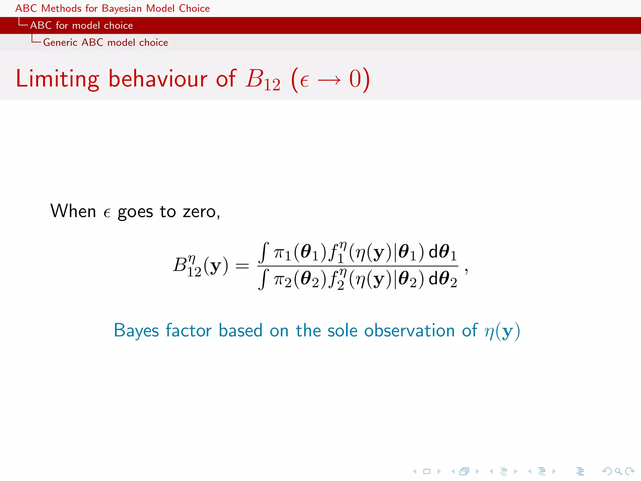
![ABC Methods for Bayesian Model Choice ABC for model choice Generic ABC model choice Limiting behaviour of B12 (under sufficiency) If η(y) sufficient statistic for both models, fi (y|θ i ) = gi (y)fiη (η(y)|θ i ) Thus η Θ1 π(θ 1 )g1 (y)f1 (η(y)|θ 1 ) dθ 1 B12 (y) = η Θ2 π(θ 2 )g2 (y)f2 (η(y)|θ 2 ) dθ 2 η g1 (y) π1 (θ 1 )f1 (η(y)|θ 1 ) dθ 1 = η g2 (y) π2 (θ 2 )f2 (η(y)|θ 2 ) dθ 2 g1 (y) η = B (y) . g2 (y) 12 [Didelot, Everitt, Johansen & Lawson, 2011]](https://image.slidesharecdn.com/zurich-110201155327-phpapp02/75/Workshop-on-Bayesian-Inference-for-Latent-Gaussian-Models-with-Applications-77-2048.jpg)
![ABC Methods for Bayesian Model Choice ABC for model choice Generic ABC model choice Limiting behaviour of B12 (under sufficiency) If η(y) sufficient statistic for both models, fi (y|θ i ) = gi (y)fiη (η(y)|θ i ) Thus η Θ1 π(θ 1 )g1 (y)f1 (η(y)|θ 1 ) dθ 1 B12 (y) = η Θ2 π(θ 2 )g2 (y)f2 (η(y)|θ 2 ) dθ 2 η g1 (y) π1 (θ 1 )f1 (η(y)|θ 1 ) dθ 1 = η g2 (y) π2 (θ 2 )f2 (η(y)|θ 2 ) dθ 2 g1 (y) η = B (y) . g2 (y) 12 [Didelot, Everitt, Johansen & Lawson, 2011] No discrepancy only when cross-model sufficiency](https://image.slidesharecdn.com/zurich-110201155327-phpapp02/75/Workshop-on-Bayesian-Inference-for-Latent-Gaussian-Models-with-Applications-78-2048.jpg)
![ABC Methods for Bayesian Model Choice ABC for model choice Generic ABC model choice Formal recovery Creating an encompassing exponential family T T f (x|θ1 , θ2 , α1 , α2 ) ∝ exp{θ1 η1 (x) + θ1 η1 (x) + α1 t1 (x) + α2 t2 (x)} leads to a sufficient statistic (η1 (x), η2 (x), t1 (x), t2 (x)) [Didelot, Everitt, Johansen & Lawson, 2011]](https://image.slidesharecdn.com/zurich-110201155327-phpapp02/75/Workshop-on-Bayesian-Inference-for-Latent-Gaussian-Models-with-Applications-81-2048.jpg)
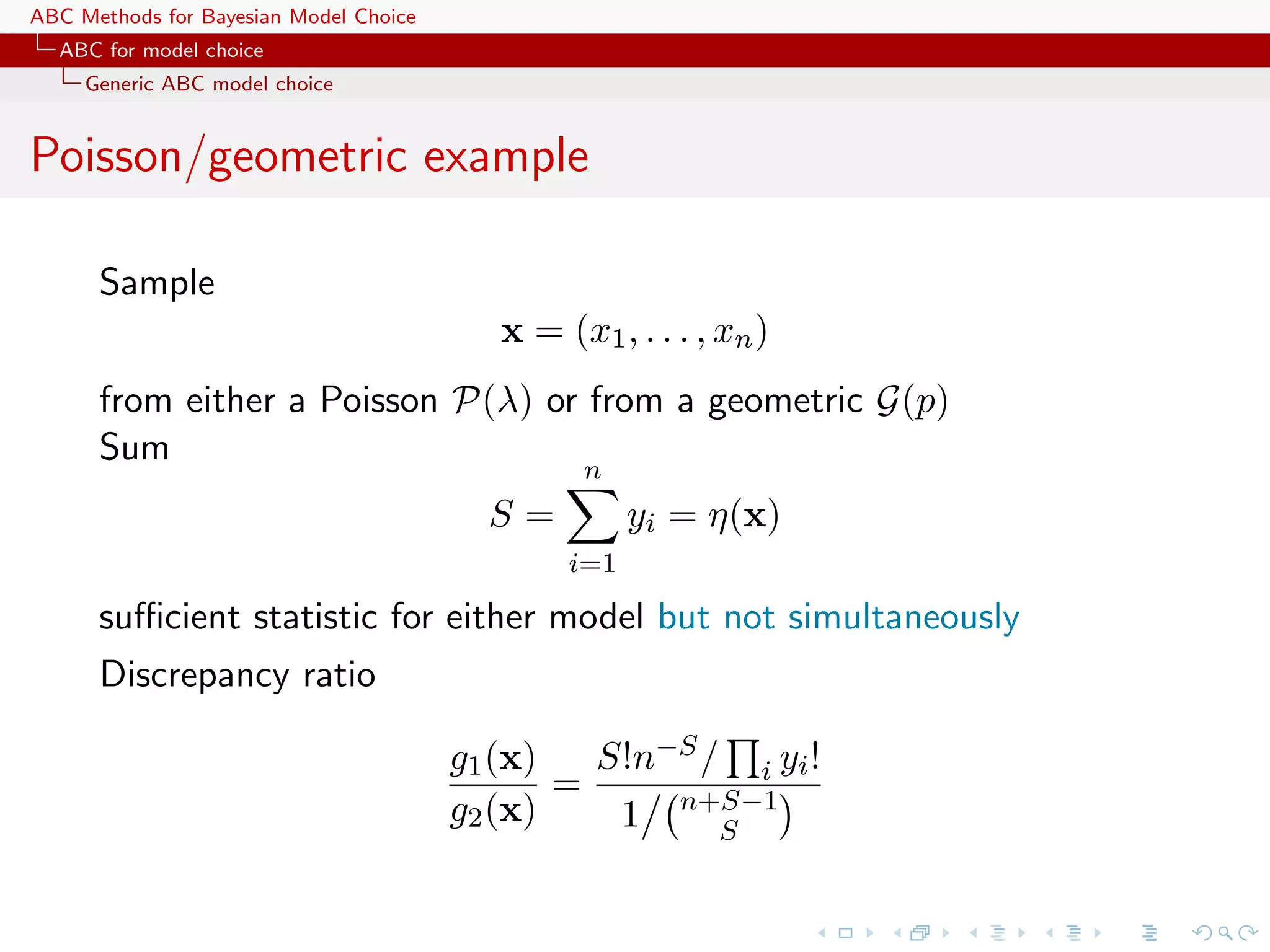
![ABC Methods for Bayesian Model Choice ABC for model choice Generic ABC model choice Formal recovery Creating an encompassing exponential family T T f (x|θ1 , θ2 , α1 , α2 ) ∝ exp{θ1 η1 (x) + θ1 η1 (x) + α1 t1 (x) + α2 t2 (x)} leads to a sufficient statistic (η1 (x), η2 (x), t1 (x), t2 (x)) [Didelot, Everitt, Johansen & Lawson, 2011] In the Poisson/geometric case, if i xi ! is added to S, no discrepancy](https://image.slidesharecdn.com/zurich-110201155327-phpapp02/75/Workshop-on-Bayesian-Inference-for-Latent-Gaussian-Models-with-Applications-82-2048.jpg)
![ABC Methods for Bayesian Model Choice ABC for model choice Generic ABC model choice Formal recovery Creating an encompassing exponential family T T f (x|θ1 , θ2 , α1 , α2 ) ∝ exp{θ1 η1 (x) + θ1 η1 (x) + α1 t1 (x) + α2 t2 (x)} leads to a sufficient statistic (η1 (x), η2 (x), t1 (x), t2 (x)) [Didelot, Everitt, Johansen & Lawson, 2011] Only applies in genuine sufficiency settings... c Inability to evaluate loss brought by summary statistics](https://image.slidesharecdn.com/zurich-110201155327-phpapp02/75/Workshop-on-Bayesian-Inference-for-Latent-Gaussian-Models-with-Applications-83-2048.jpg)
![ABC Methods for Bayesian Model Choice ABC for model choice Generic ABC model choice Meaning of the ABC-Bayes factor ‘This is also why focus on model discrimination typically (...) proceeds by (...) accepting that the Bayes Factor that one obtains is only derived from the summary statistics and may in no way correspond to that of the full model.’ [Scott Sisson, Jan. 31, 2011, ’Og]](https://image.slidesharecdn.com/zurich-110201155327-phpapp02/75/Workshop-on-Bayesian-Inference-for-Latent-Gaussian-Models-with-Applications-84-2048.jpg)
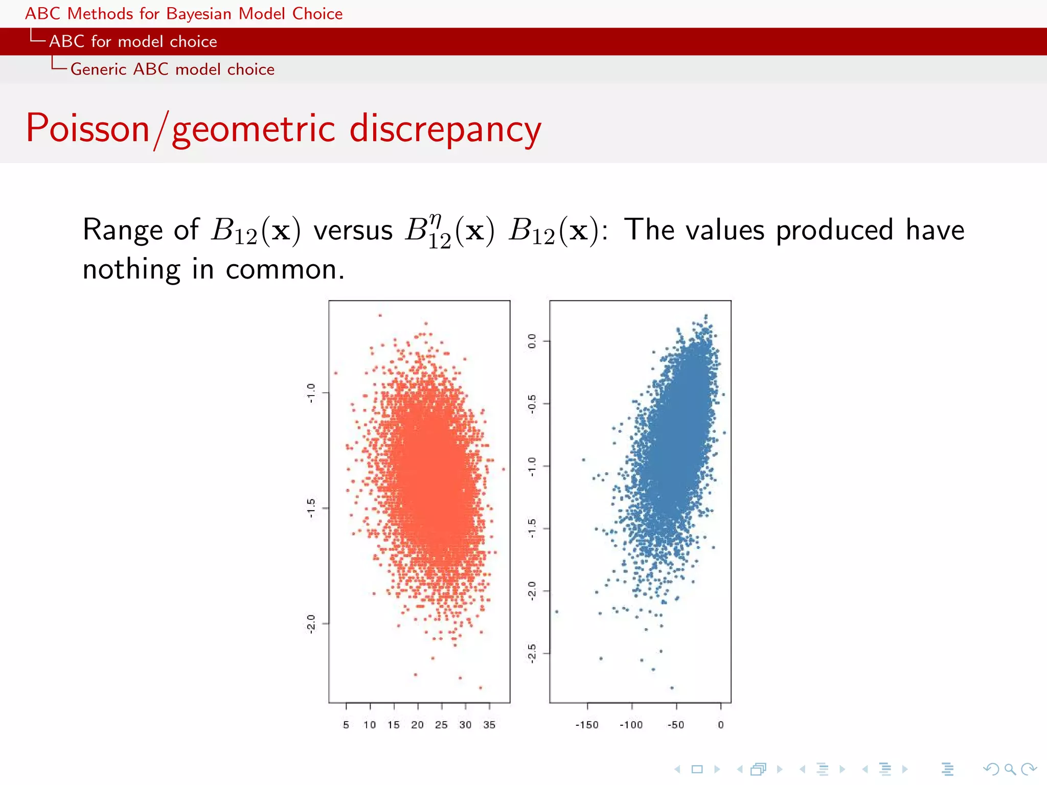
![ABC Methods for Bayesian Model Choice ABC for model choice Generic ABC model choice Meaning of the ABC-Bayes factor ‘This is also why focus on model discrimination typically (...) proceeds by (...) accepting that the Bayes Factor that one obtains is only derived from the summary statistics and may in no way correspond to that of the full model.’ [Scott Sisson, Jan. 31, 2011, ’Og] In the Poisson/geometric case, if E[yi ] = θ0 > 0, η (θ0 + 1)2 −θ0 lim B12 (y) = e n→∞ θ0](https://image.slidesharecdn.com/zurich-110201155327-phpapp02/75/Workshop-on-Bayesian-Inference-for-Latent-Gaussian-Models-with-Applications-85-2048.jpg)
![ABC Methods for Bayesian Model Choice ABC for model choice Generic ABC model choice MA(q) divergence 1.0 1.0 1.0 1.0 0.8 0.8 0.8 0.8 0.6 0.6 0.6 0.6 0.4 0.4 0.4 0.4 0.2 0.2 0.2 0.2 0.0 0.0 0.0 0.0 1 2 1 2 1 2 1 2 Evolution [against ] of ABC Bayes factor, in terms of frequencies of visits to models MA(1) (left) and MA(2) (right) when equal to 10, 1, .1, .01% quantiles on insufficient autocovariance distances. Sample of 50 points from a MA(2) with θ1 = 0.6, θ2 = 0.2. True Bayes factor equal to 17.71.](https://image.slidesharecdn.com/zurich-110201155327-phpapp02/75/Workshop-on-Bayesian-Inference-for-Latent-Gaussian-Models-with-Applications-86-2048.jpg)
![ABC Methods for Bayesian Model Choice ABC for model choice Generic ABC model choice MA(q) divergence 1.0 1.0 1.0 1.0 0.8 0.8 0.8 0.8 0.6 0.6 0.6 0.6 0.4 0.4 0.4 0.4 0.2 0.2 0.2 0.2 0.0 0.0 0.0 0.0 1 2 1 2 1 2 1 2 Evolution [against ] of ABC Bayes factor, in terms of frequencies of visits to models MA(1) (left) and MA(2) (right) when equal to 10, 1, .1, .01% quantiles on insufficient autocovariance distances. Sample of 50 points from a MA(1) model with θ1 = 0.6. True Bayes factor B21 equal to .004.](https://image.slidesharecdn.com/zurich-110201155327-phpapp02/75/Workshop-on-Bayesian-Inference-for-Latent-Gaussian-Models-with-Applications-87-2048.jpg)
![ABC Methods for Bayesian Model Choice ABC for model choice Generic ABC model choice Further comments ‘There should be the possibility that for the same model, but different (non-minimal) [summary] statistics (so ∗ different η’s: η1 and η1 ) the ratio of evidences may no longer be equal to one.’ [Michael Stumpf, Jan. 28, 2011, ’Og] Using different summary statistics [on different models] may indicate the loss of information brought by each set but agreement does not lead to trustworthy approximations.](https://image.slidesharecdn.com/zurich-110201155327-phpapp02/75/Workshop-on-Bayesian-Inference-for-Latent-Gaussian-Models-with-Applications-88-2048.jpg)
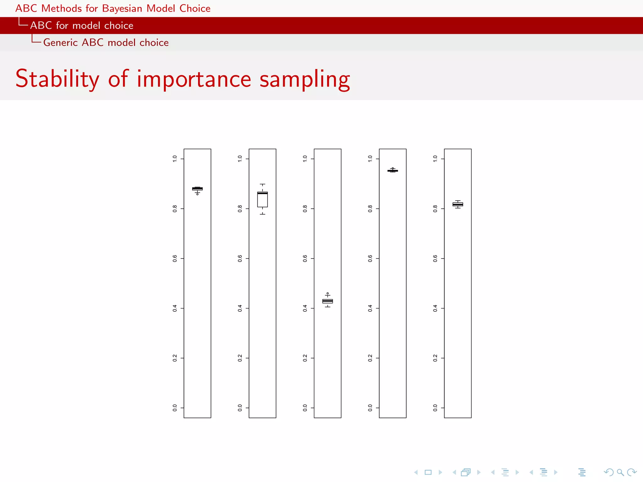
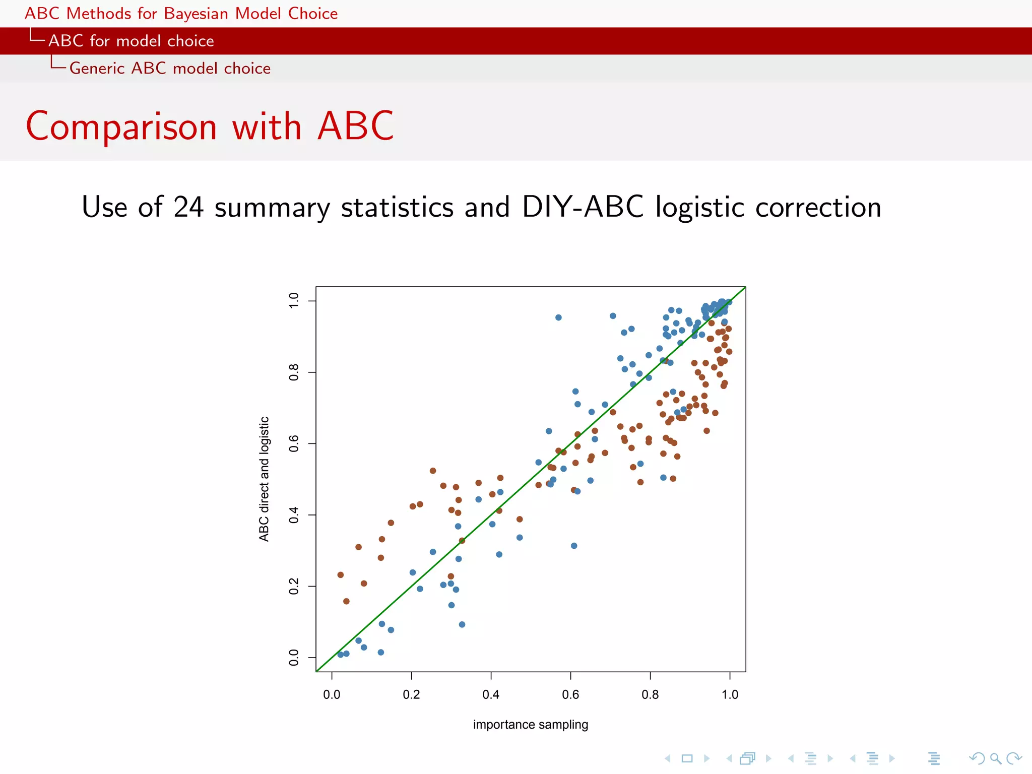
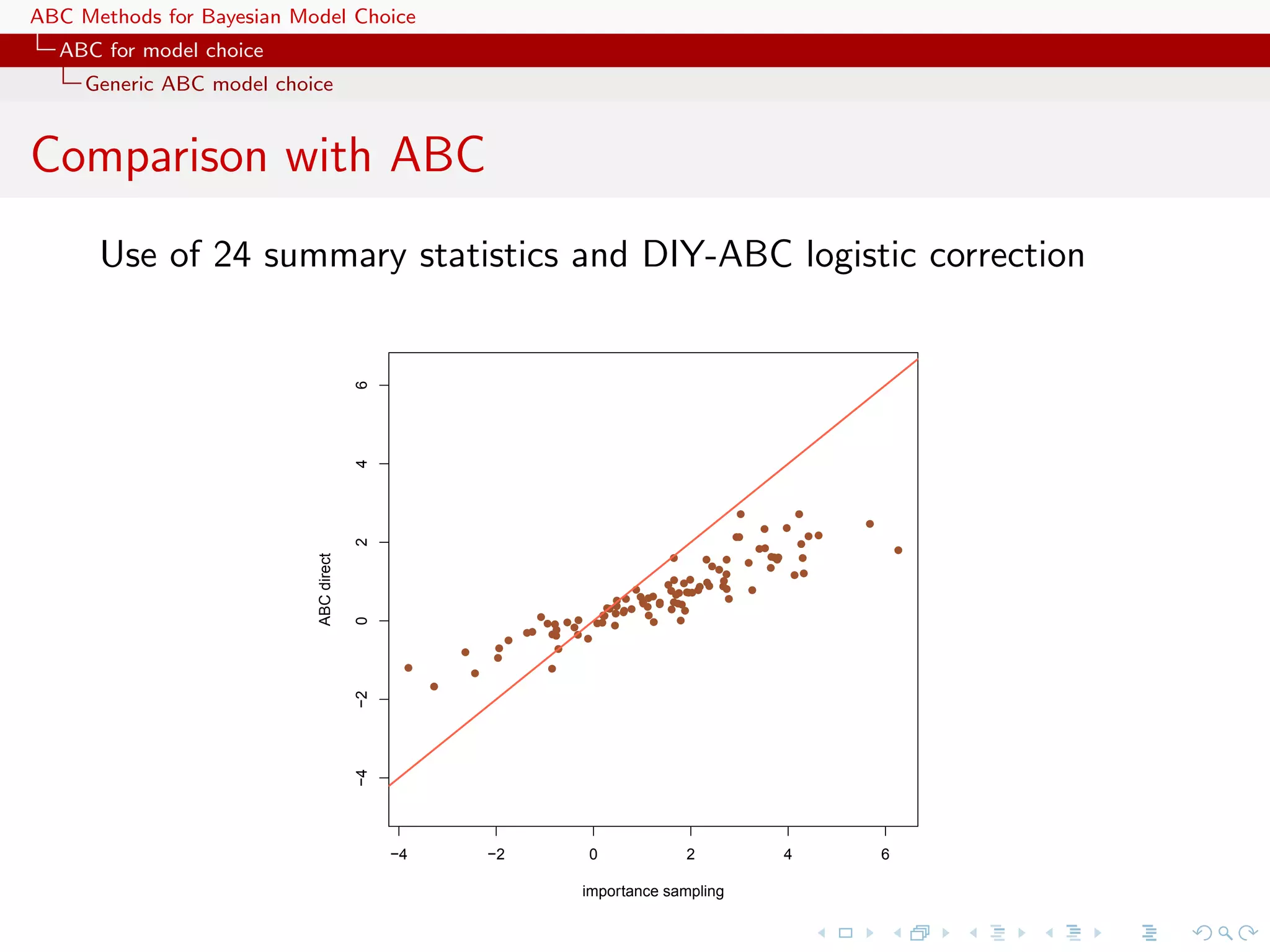
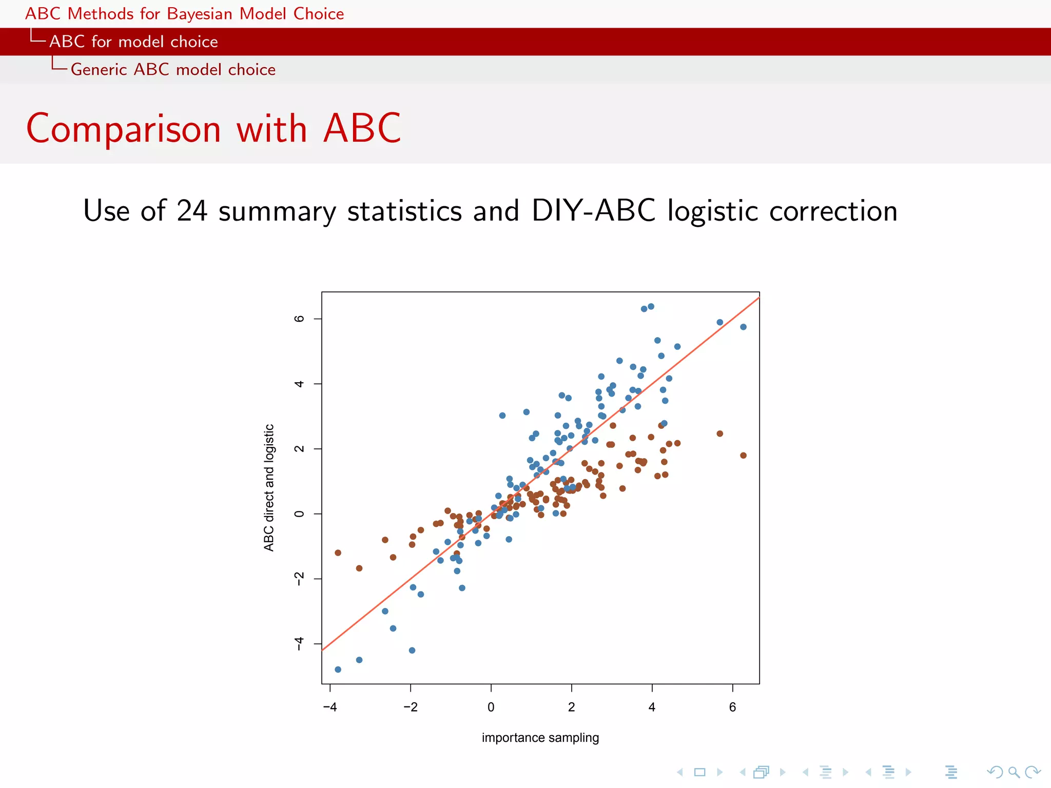
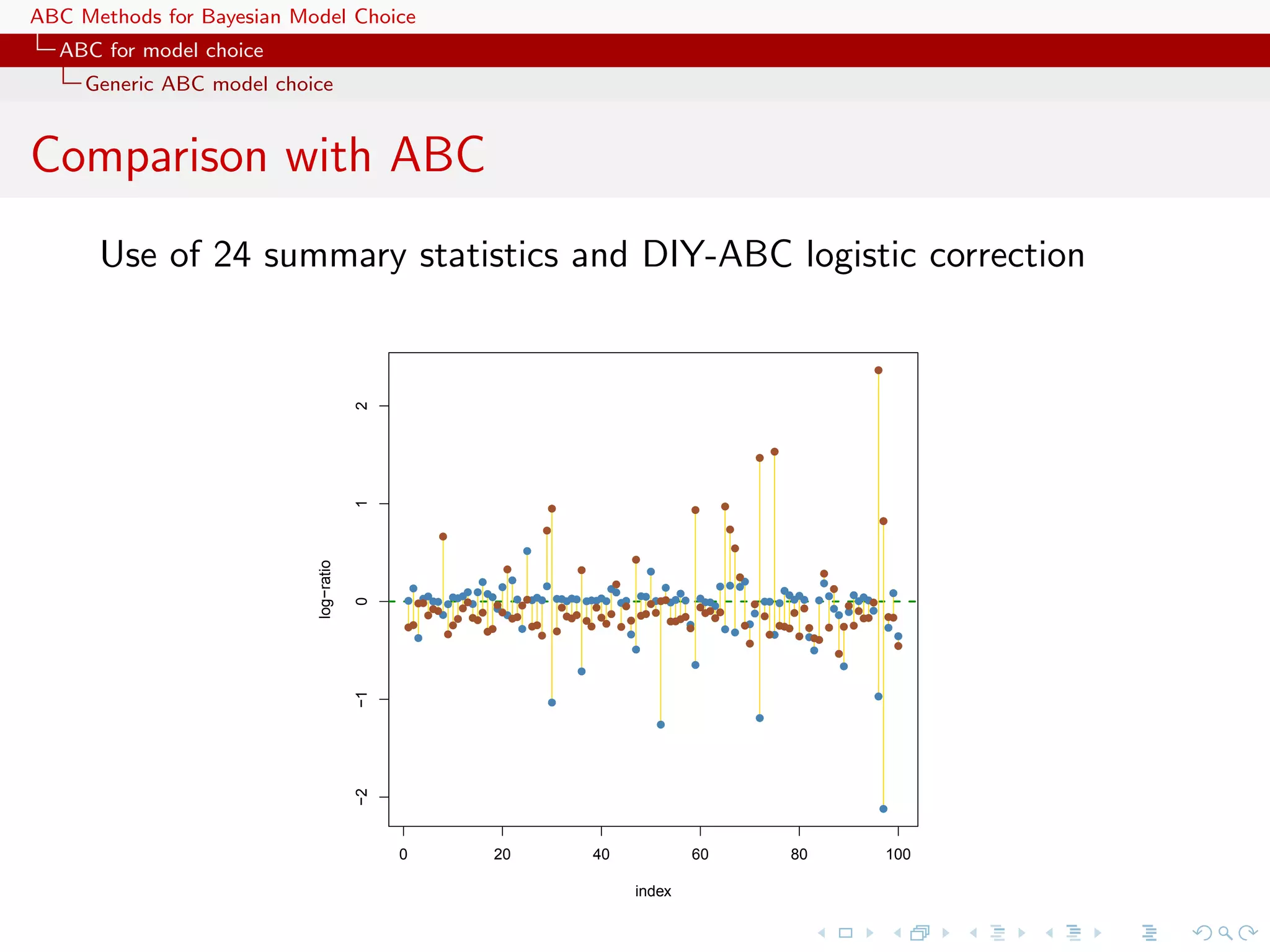
![ABC Methods for Bayesian Model Choice ABC for model choice Generic ABC model choice A population genetics evaluation Population genetics example with 3 populations 2 scenari 15 individuals 5 loci single mutation parameter 24 summary statistics 2 million ABC proposal importance [tree] sampling alternative](https://image.slidesharecdn.com/zurich-110201155327-phpapp02/75/Workshop-on-Bayesian-Inference-for-Latent-Gaussian-Models-with-Applications-90-2048.jpg)
![ABC Methods for Bayesian Model Choice ABC for model choice Generic ABC model choice A population genetics evaluation Population genetics example with 3 populations 2 scenari 15 individuals 5 loci single mutation parameter 24 summary statistics 2 million ABC proposal importance [tree] sampling alternative](https://image.slidesharecdn.com/zurich-110201155327-phpapp02/75/Workshop-on-Bayesian-Inference-for-Latent-Gaussian-Models-with-Applications-91-2048.jpg)
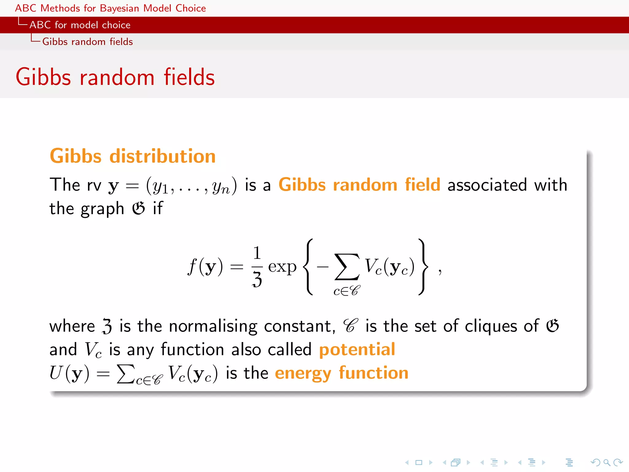
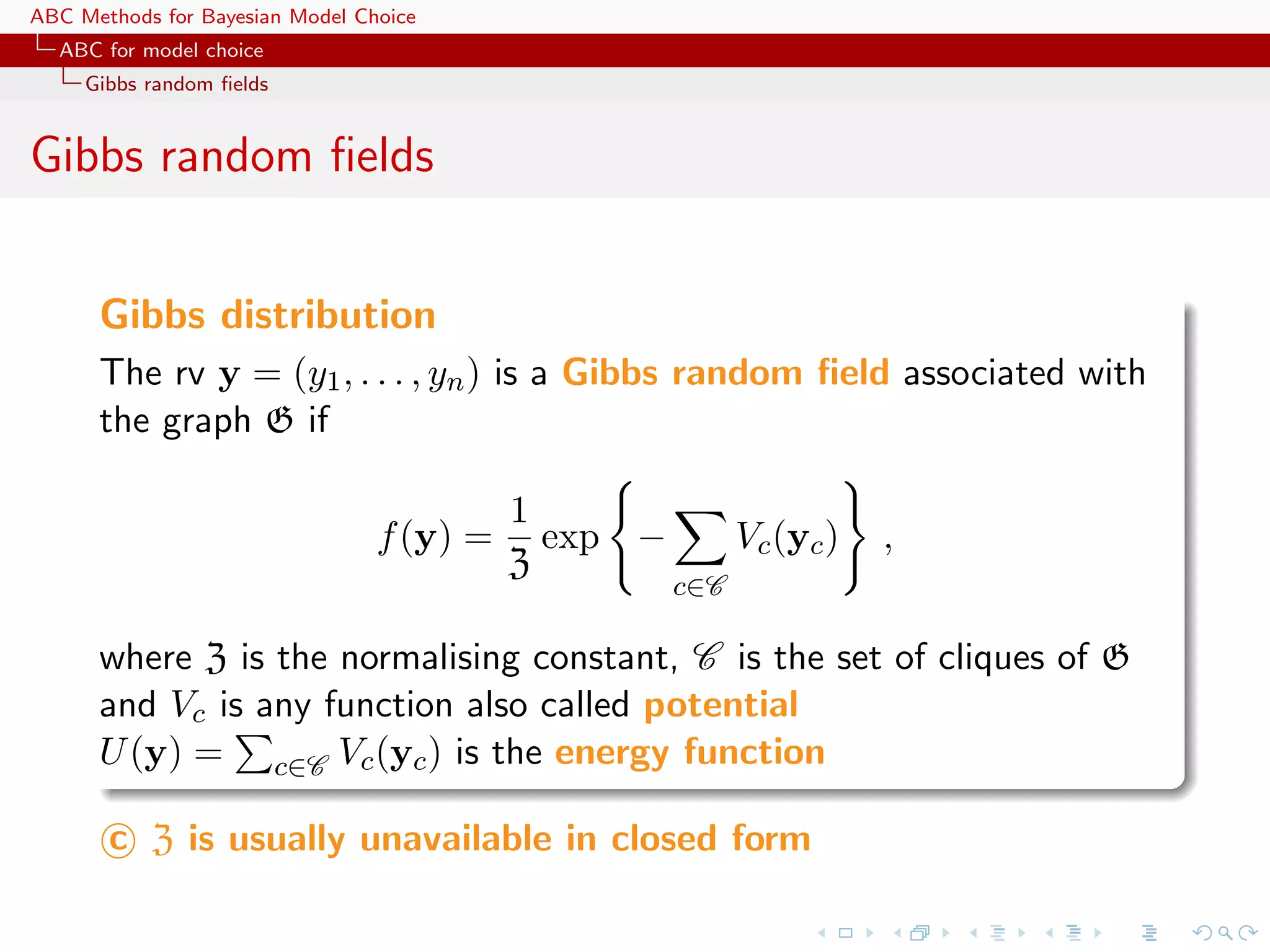
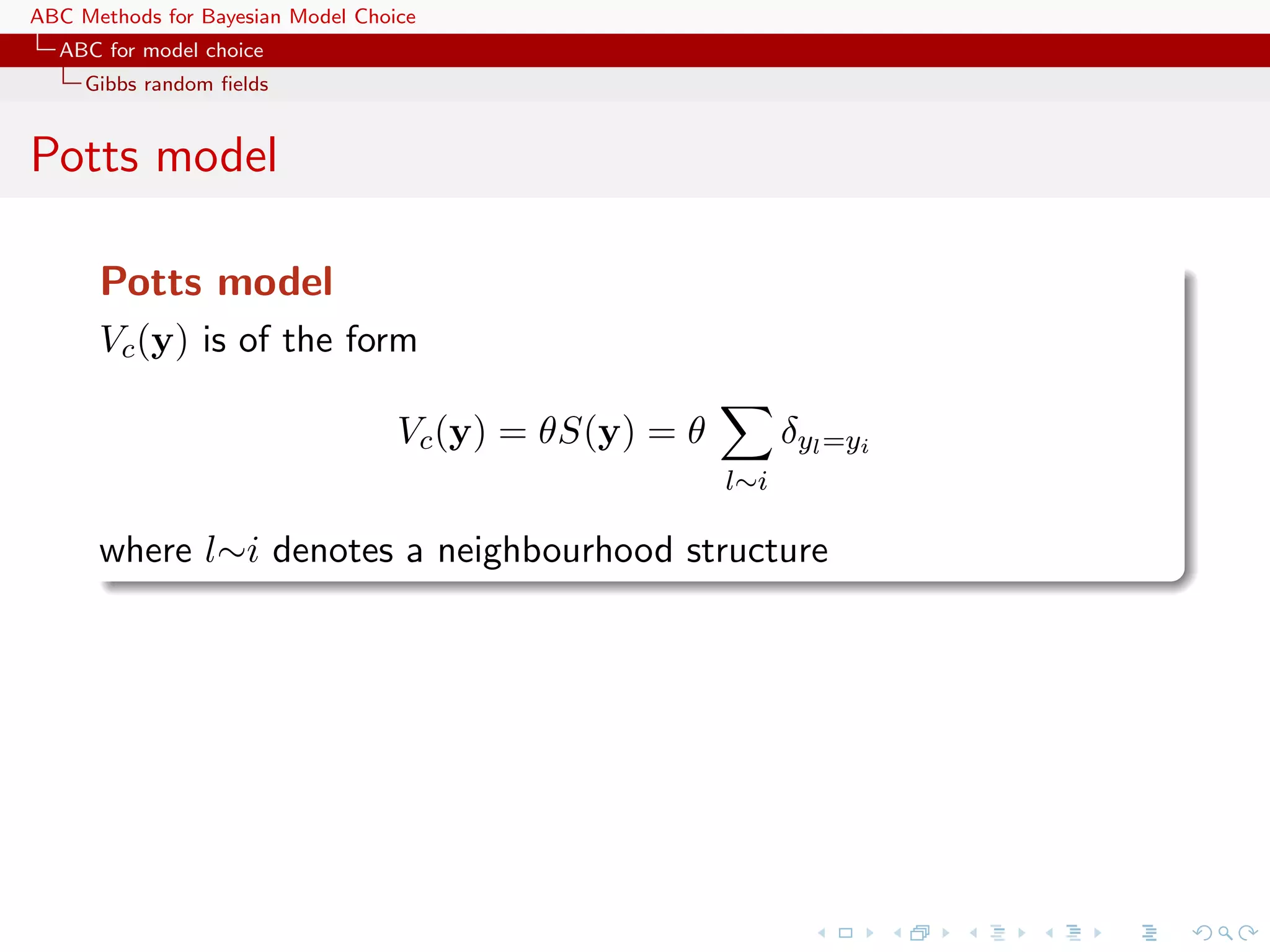
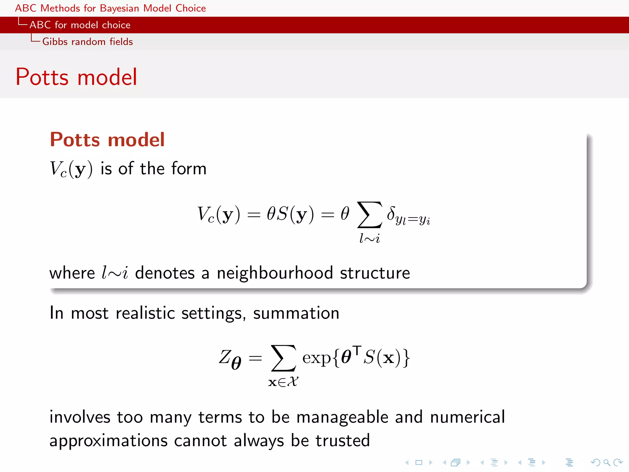
![ABC Methods for Bayesian Model Choice ABC for model choice Generic ABC model choice The only safe cases Besides specific models like Gibbs random fields, using distances over the data itself escapes the discrepancy... [Toni & Stumpf, 2010;Sousa et al., 2009]](https://image.slidesharecdn.com/zurich-110201155327-phpapp02/75/Workshop-on-Bayesian-Inference-for-Latent-Gaussian-Models-with-Applications-97-2048.jpg)
![ABC Methods for Bayesian Model Choice ABC for model choice Generic ABC model choice The only safe cases Besides specific models like Gibbs random fields, using distances over the data itself escapes the discrepancy... [Toni & Stumpf, 2010;Sousa et al., 2009] ...and so does the use of more informal model fitting measures [Ratmann, Andrieu, Richardson and Wiujf, 2009]](https://image.slidesharecdn.com/zurich-110201155327-phpapp02/75/Workshop-on-Bayesian-Inference-for-Latent-Gaussian-Models-with-Applications-98-2048.jpg)

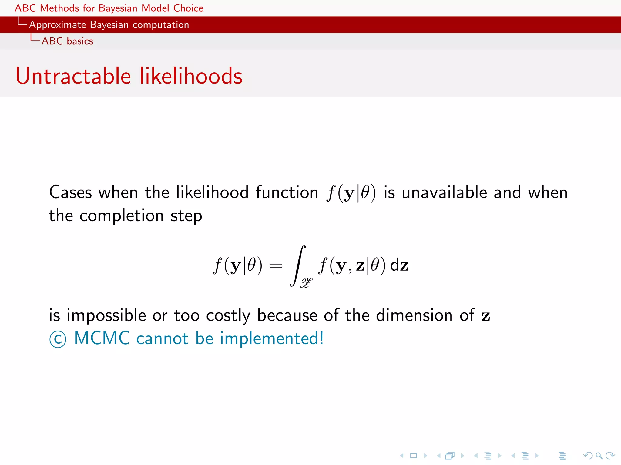
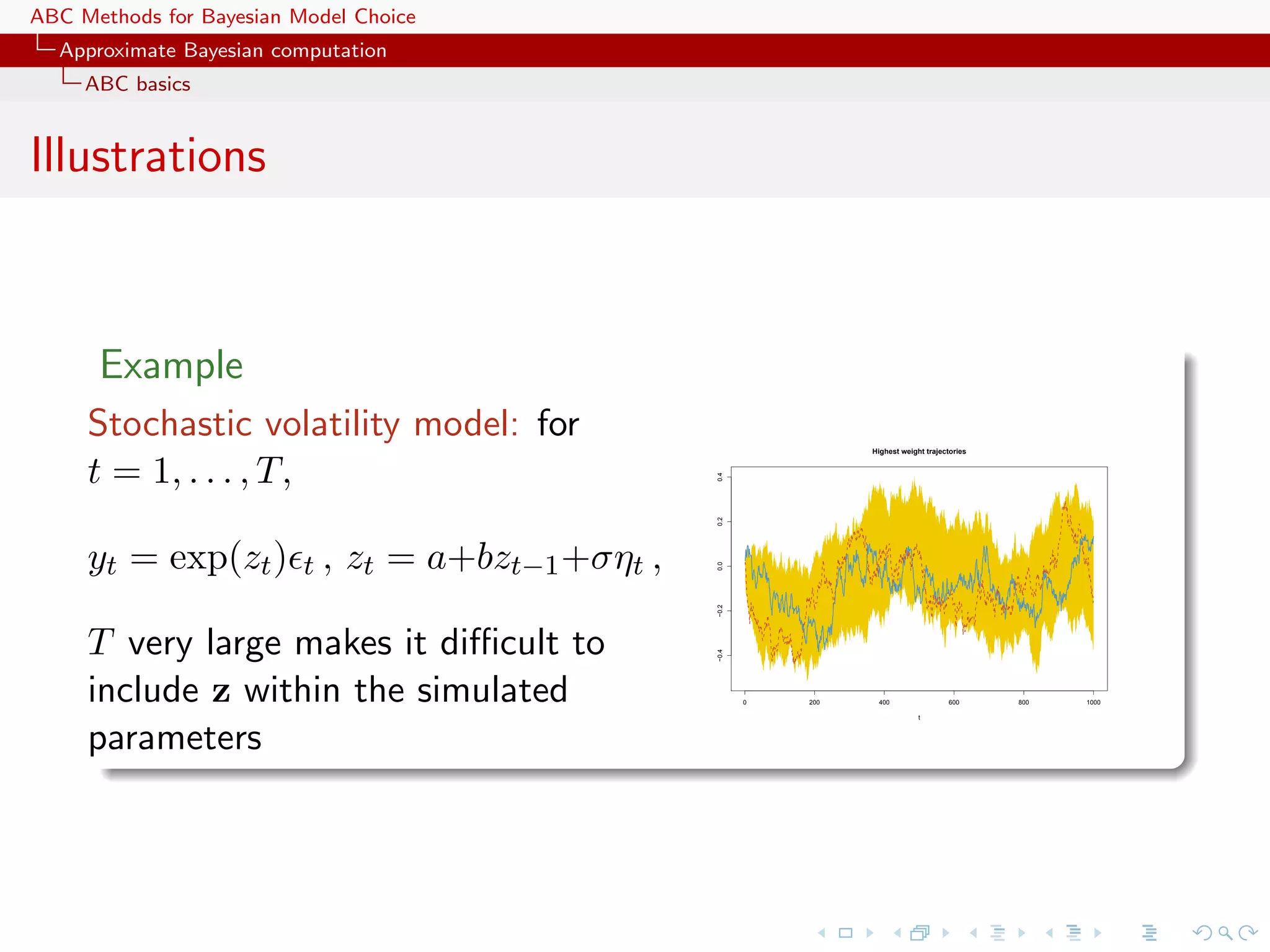
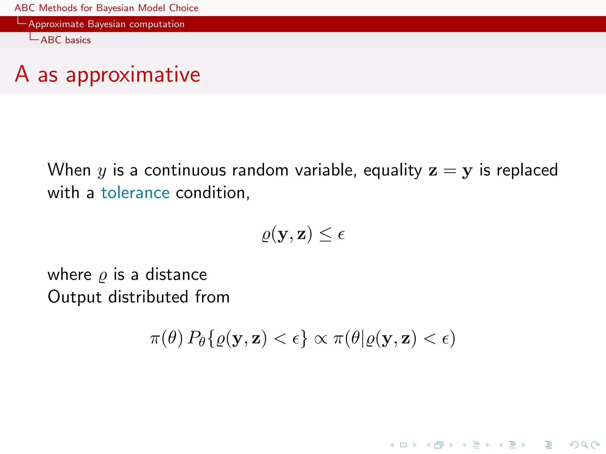
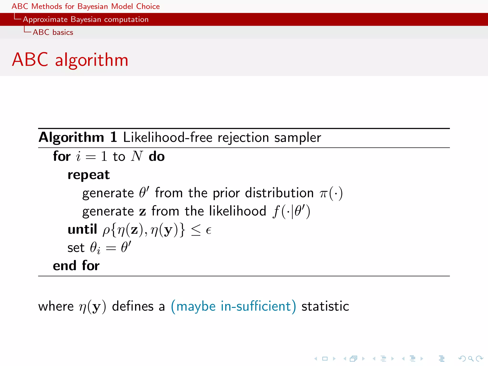
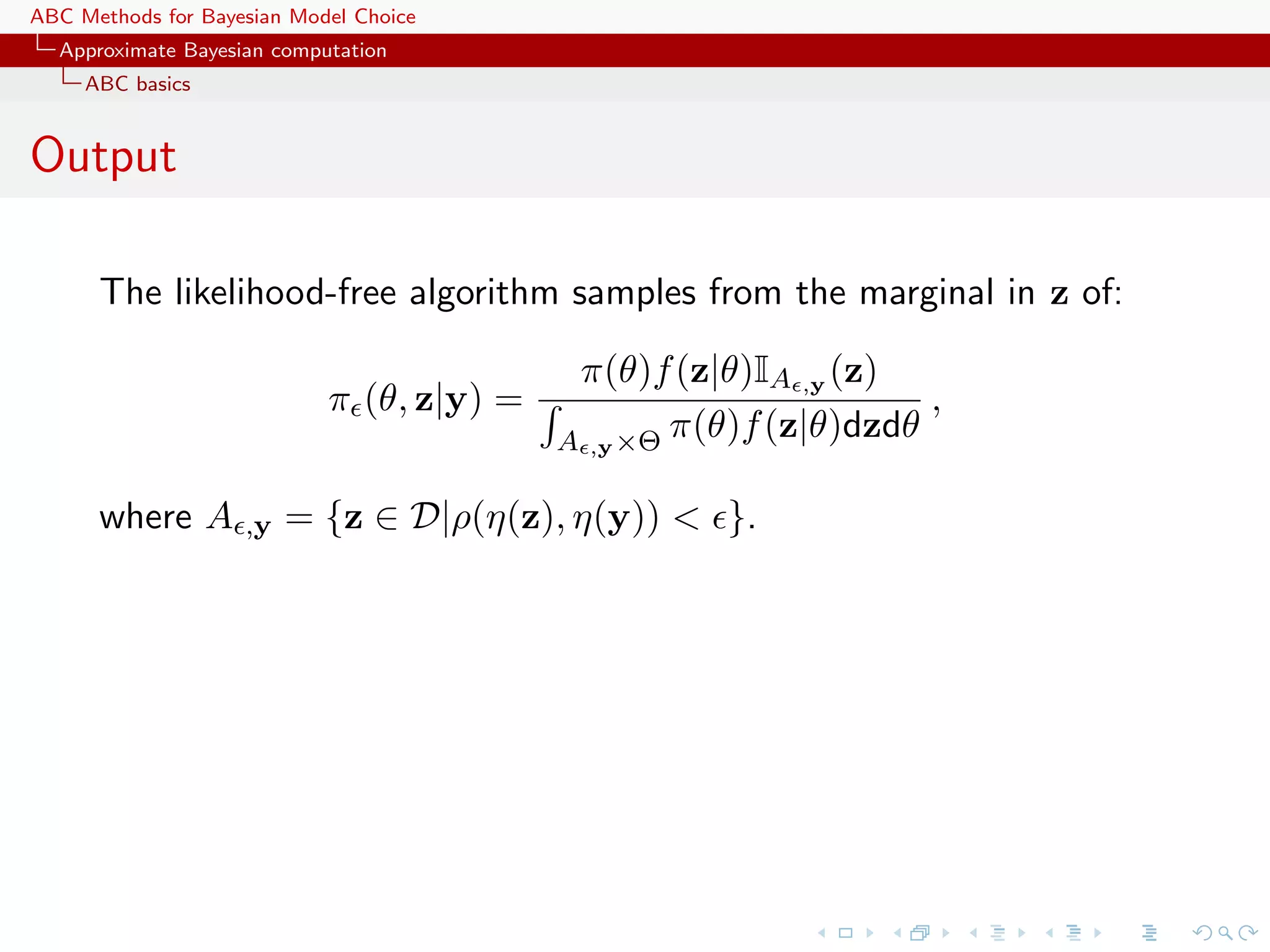
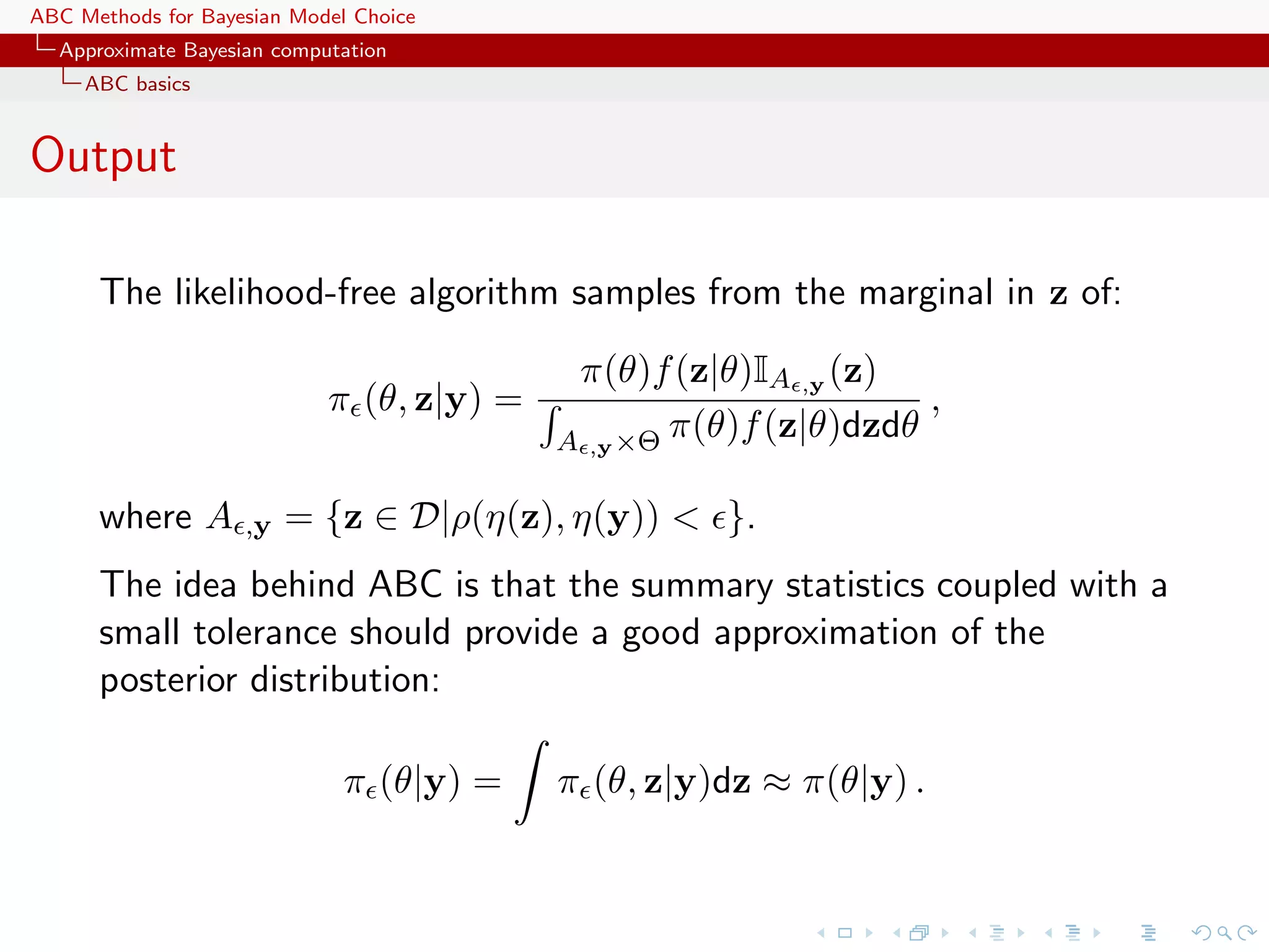
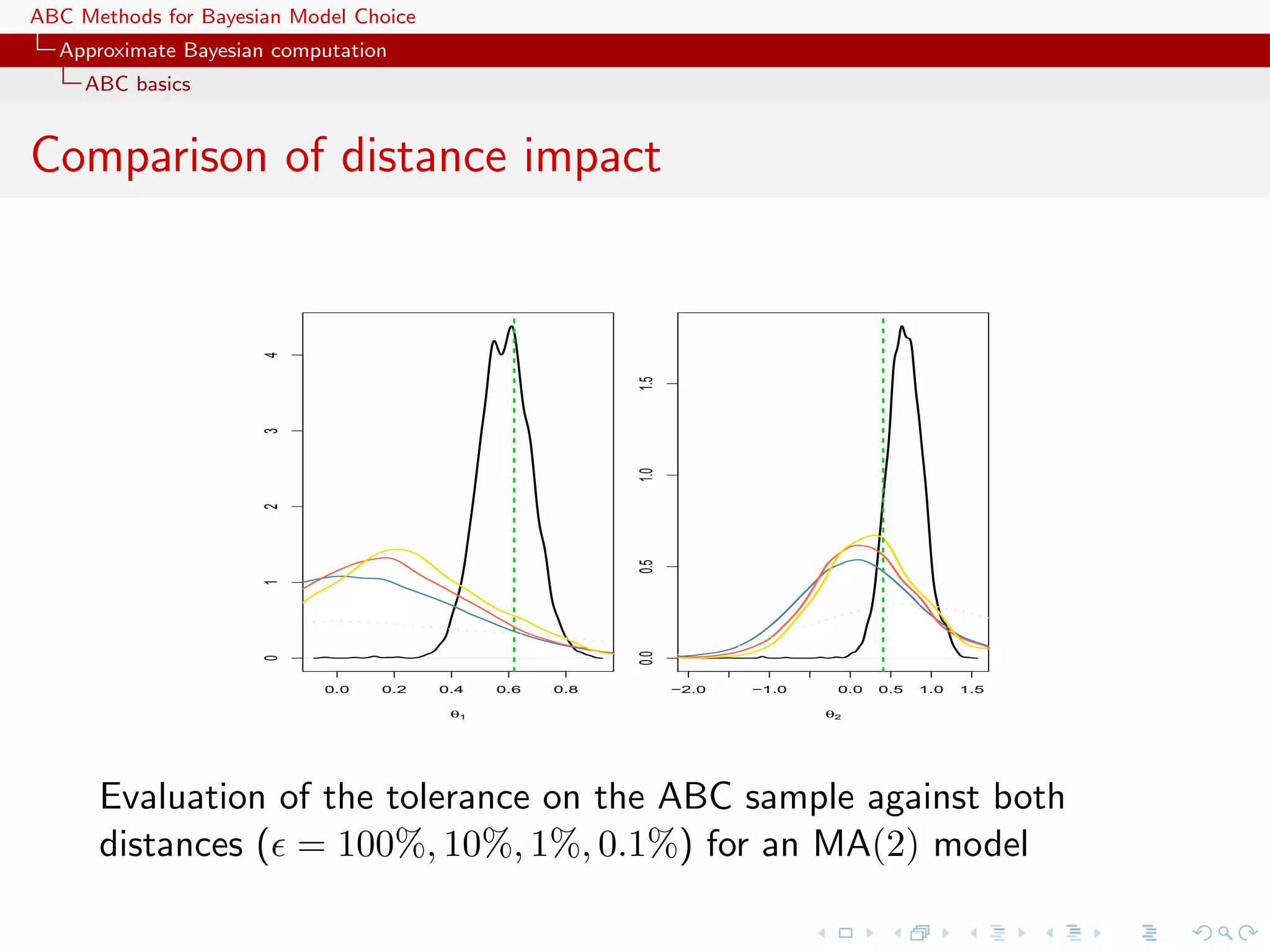
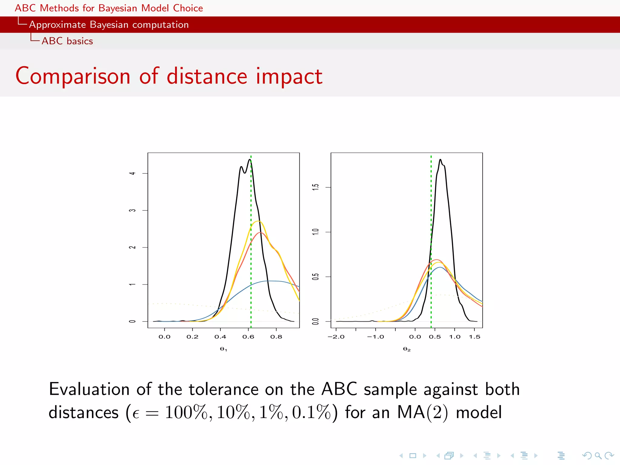
ABC methods provide a way to perform Bayesian inference when the likelihood function is intractable or impossible to compute directly. The basic ABC algorithm works by simulating parameters from the prior and simulating data from those parameters, accepting the parameters if the simulated data is "close" to the actual observed data according to some distance measure and tolerance level. Later advances include ABC-MCMC which uses an MCMC approach to sample from the posterior, and ABC-NP which adjusts the parameters to better match the observed data rather than rejecting simulations. Other variants such as ABC-SMC and ABC-μ extend the framework to include sequential Monte Carlo methods or jointly model the intractable parameters. Overall, ABC methods provide a