Downloaded 53 times

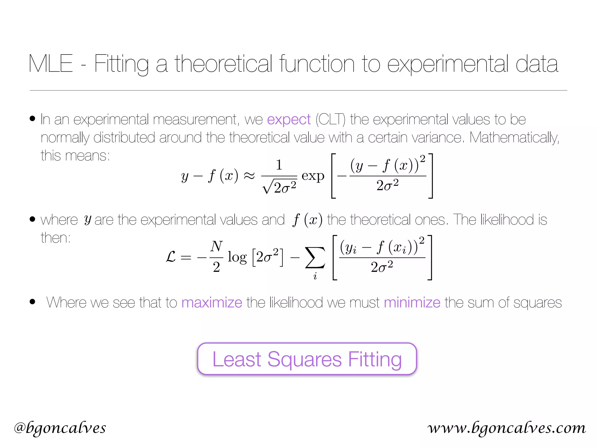
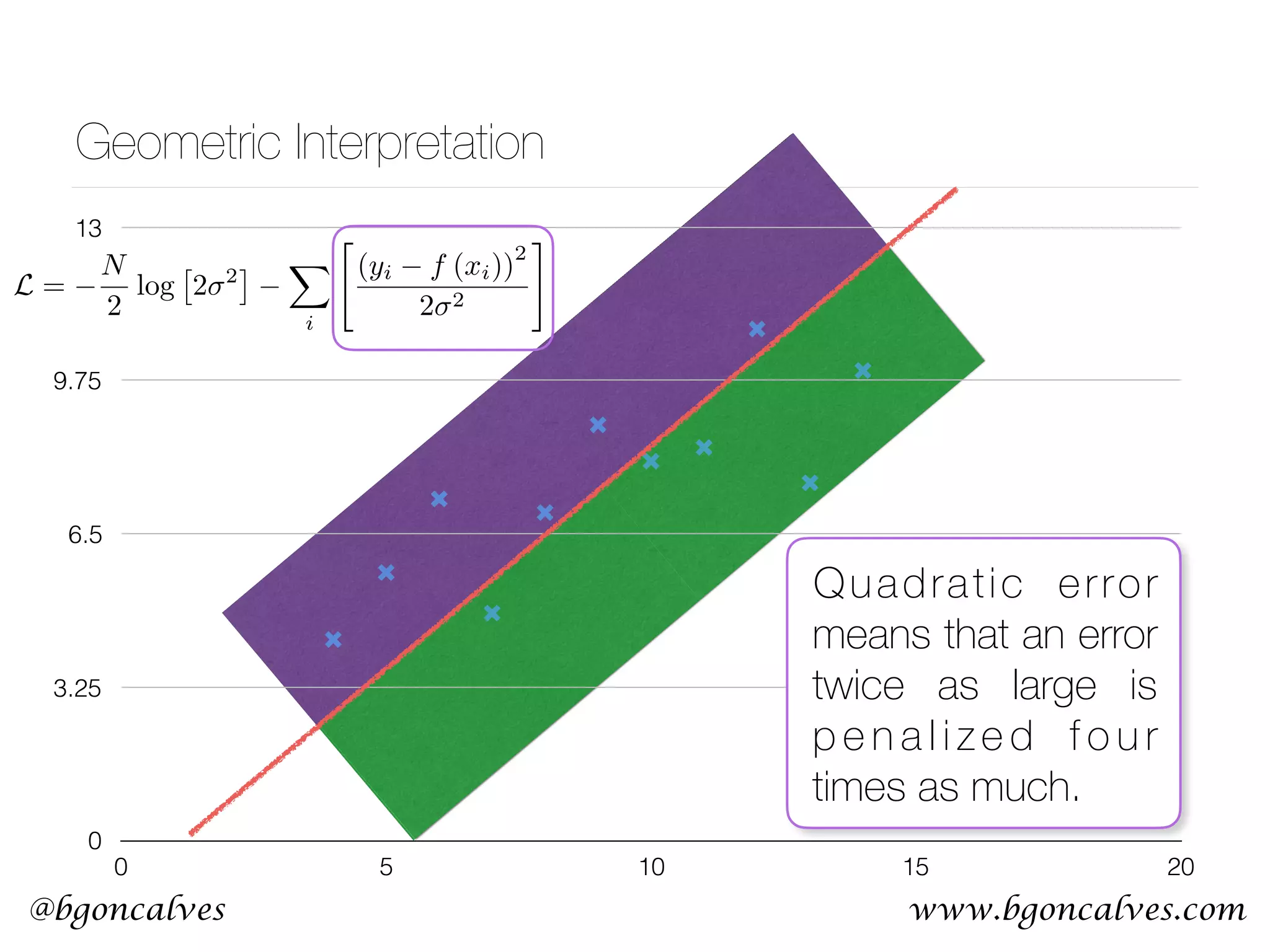
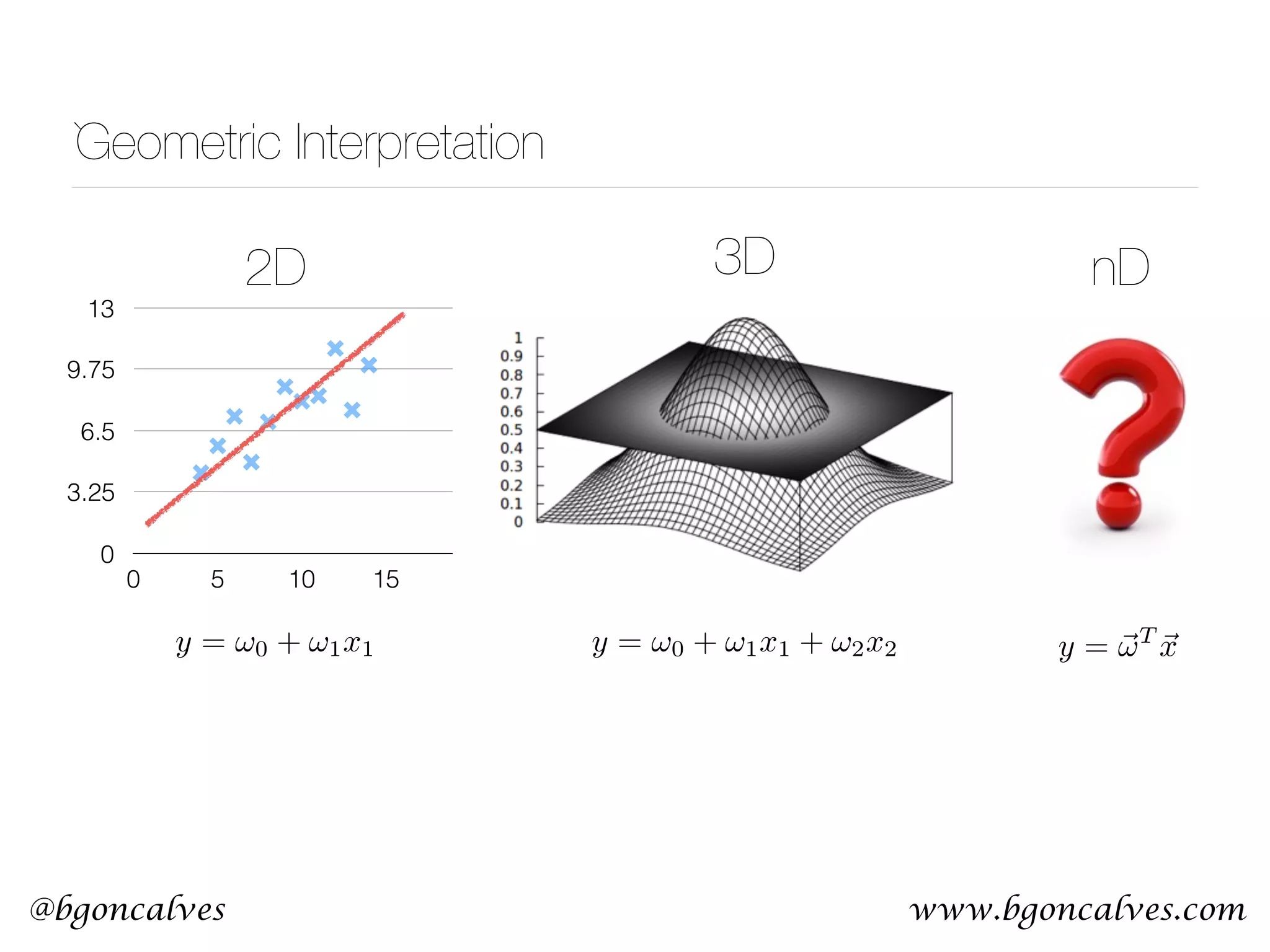
![www.bgoncalves.com@bgoncalves MLE - Linear Regression • Let’s say we want to fit a straight line to a set of points: • The Likelihood function then becomes:
• With partial derivatives:
• Setting to zero and solving for and : y = w · x + b L = N 2 log ⇥ 2 2 ⇤ X i " (yi w · xi b) 2 2 2 # @L @w = X i [2xi (yi w · xi b)] @L @b = X i [(yi w · xi b)] ˆw = P i (xi hxi) (yi hyi) P i (xi hxi) 2 ˆb = hyi ˆwhxi ˆw ˆb](https://image.slidesharecdn.com/machinelearningcopy-161201153202/75/A-practical-Introduction-to-Machine-s-Learning-15-2048.jpg)
![@bgoncalves MLE for Linear Regression from __future__ import print_function import sys import numpy as np from scipy import optimize data = np.loadtxt(sys.argv[1]) x = data.T[0] y = data.T[1] meanx = np.mean(x) meany = np.mean(y) w = np.sum((x-meanx)*(y-meany))/np.sum((x-meanx)**2) b = meany-w*meanx print(w, b) #We can also optimize the Likelihood expression directly def likelihood(w): global x, y sigma = 1.0 w, b = w return np.sum((y-w*x-b)**2)/(2*sigma) w, b = optimize.fmin_bfgs(likelihood, [1.0, 1.0]) print(w, b) MLElinear.py](https://image.slidesharecdn.com/machinelearningcopy-161201153202/75/A-practical-Introduction-to-Machine-s-Learning-16-2048.jpg)

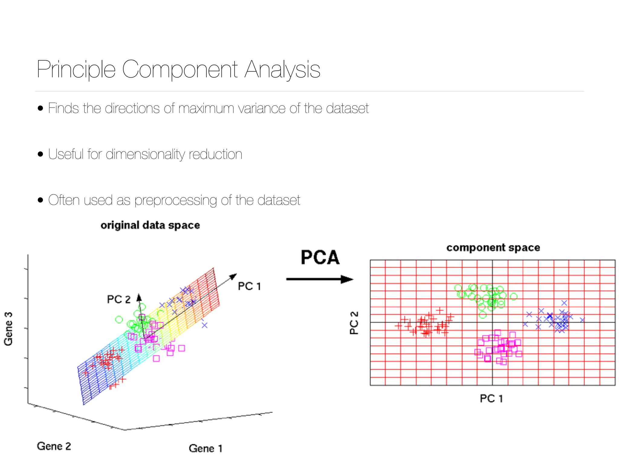
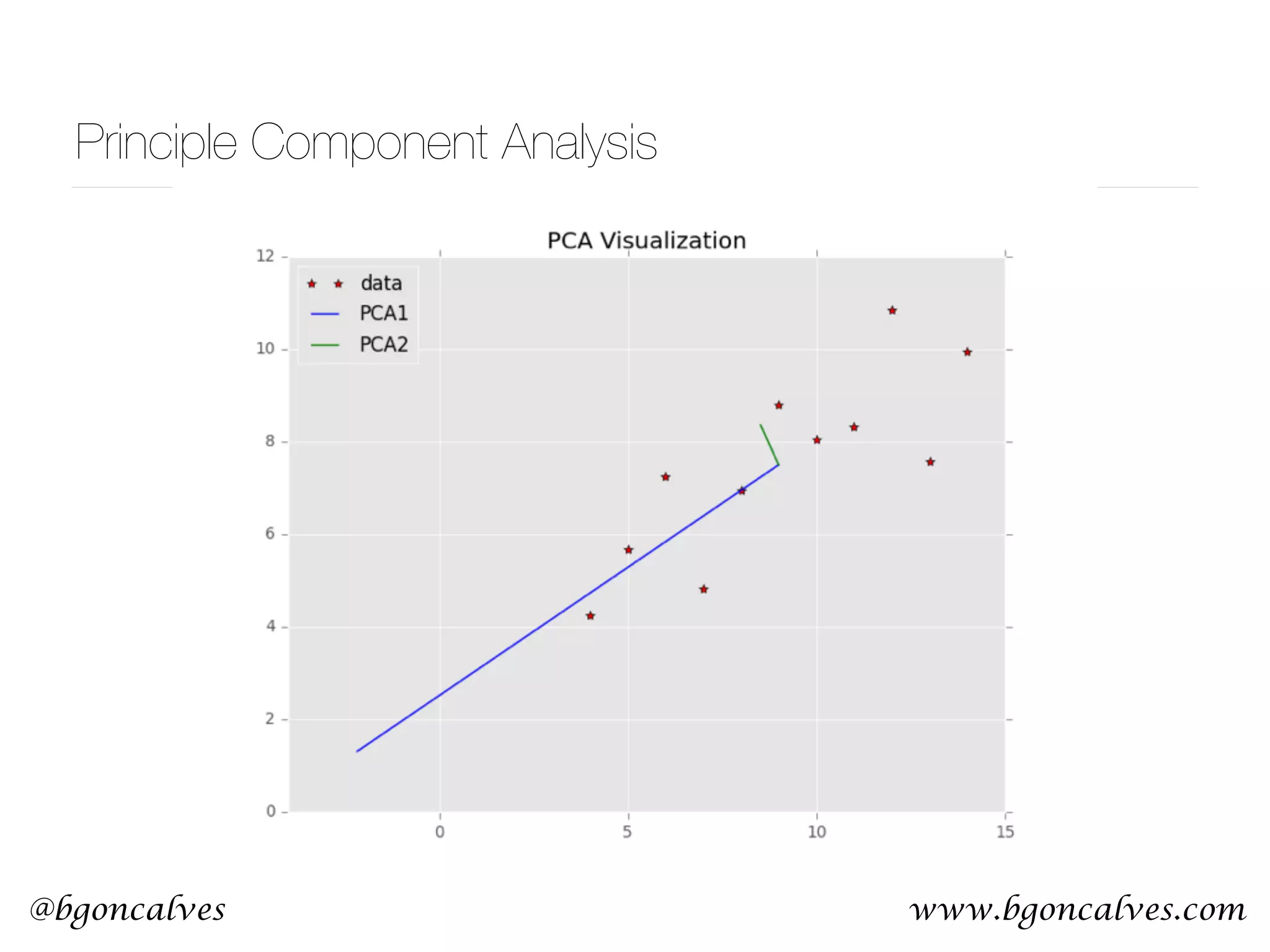
![@bgoncalves Principle Component Analysis from __future__ import print_function import sys from sklearn.decomposition import PCA import numpy as np import matplotlib.pyplot as plt data = np.loadtxt(sys.argv[1]) x = data.T[0] y = data.T[1] pca = PCA() pca.fit(data) meanX = np.mean(x) meanY = np.mean(y) plt.style.use('ggplot') plt.plot(x, y, 'r*') plt.plot([meanX, meanX+pca.components_[0][0]*pca.explained_variance_[0]], [meanY, meanY+pca.components_[0][1]*pca.explained_variance_[0]], 'b-') plt.plot([meanX, meanX+pca.components_[1][0]*pca.explained_variance_[1]], [meanY, meanY+pca.components_[1][1]*pca.explained_variance_[1]], 'g-') plt.title('PCA Visualization') plt.legend(['data', 'PCA1', 'PCA2'], loc=2) plt.savefig('PCA.png') PCA.py](https://image.slidesharecdn.com/machinelearningcopy-161201153202/75/A-practical-Introduction-to-Machine-s-Learning-37-2048.jpg)
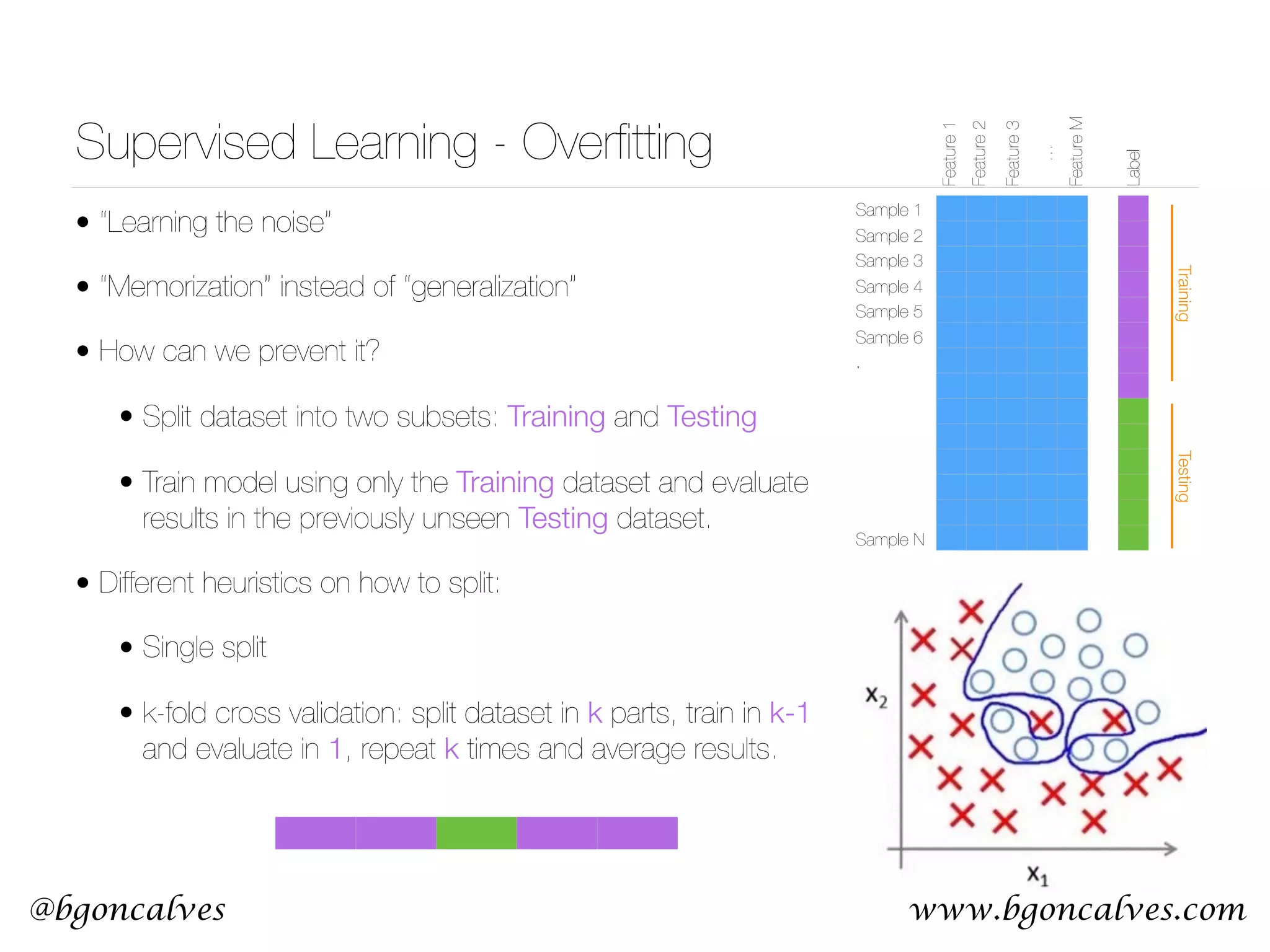
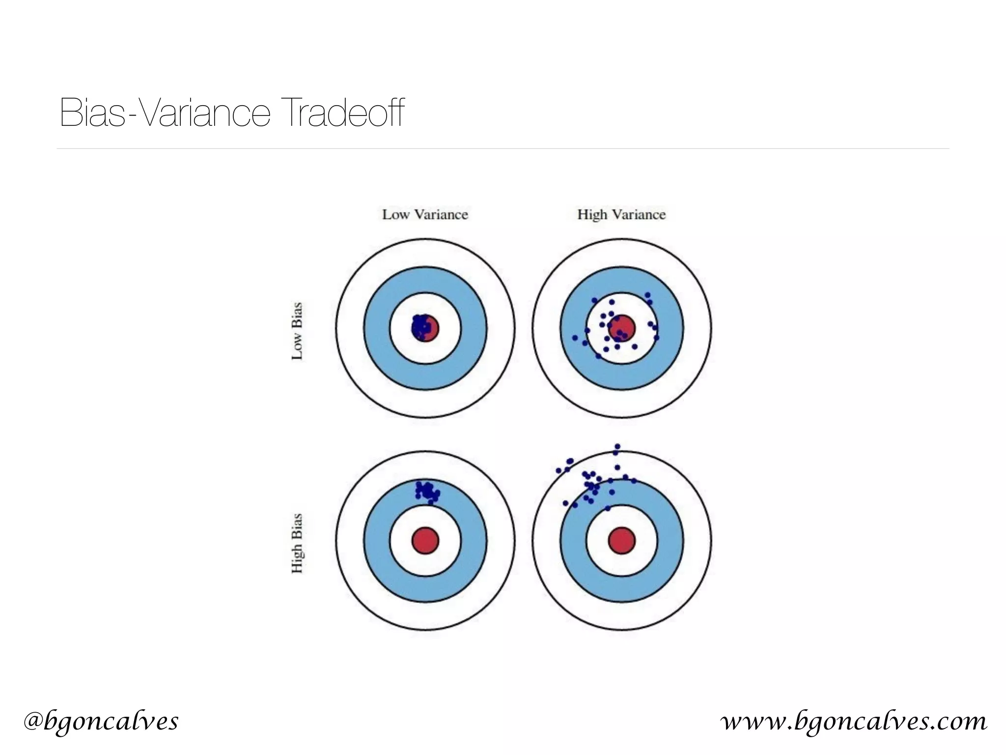
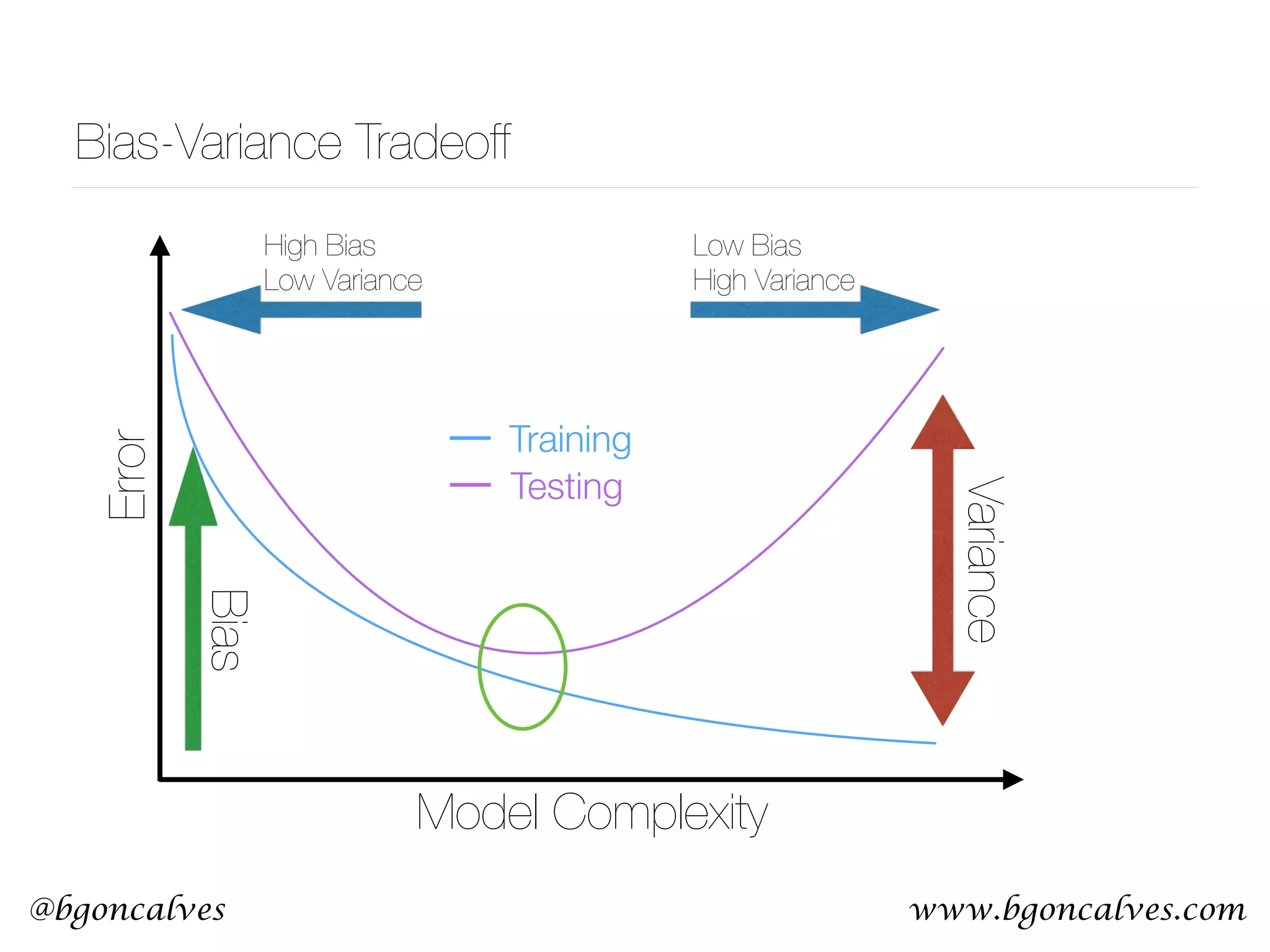
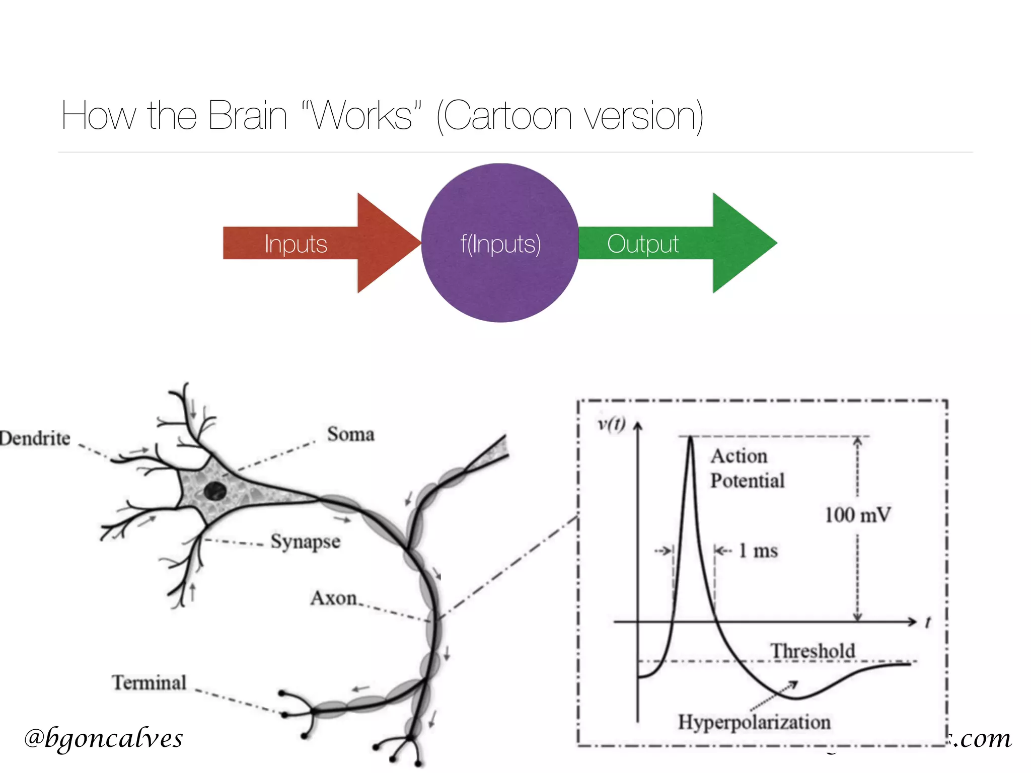
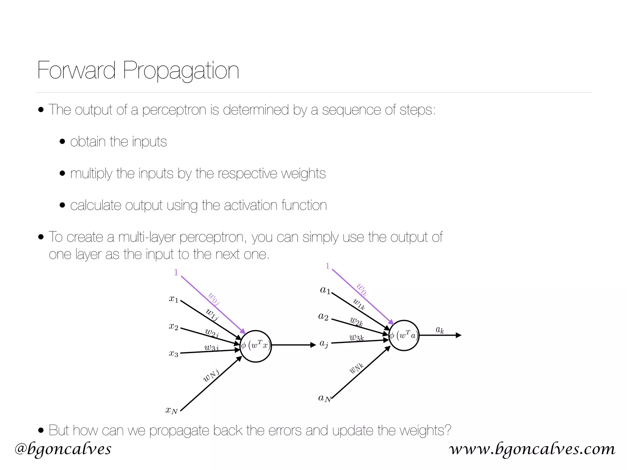
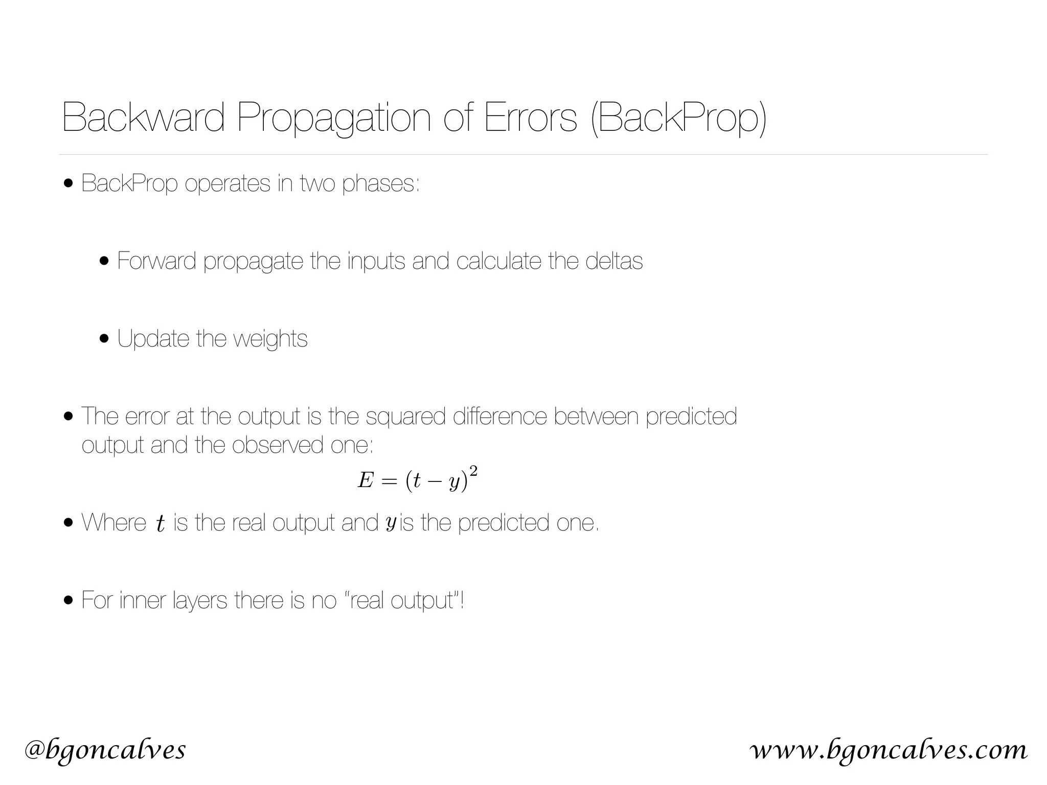

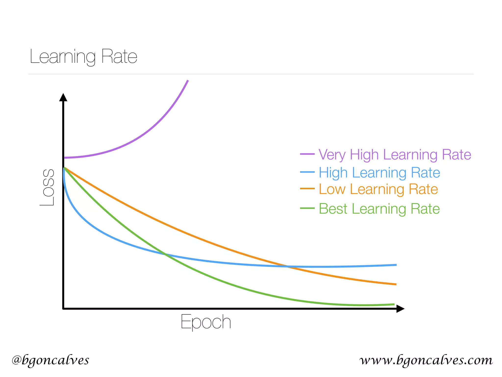


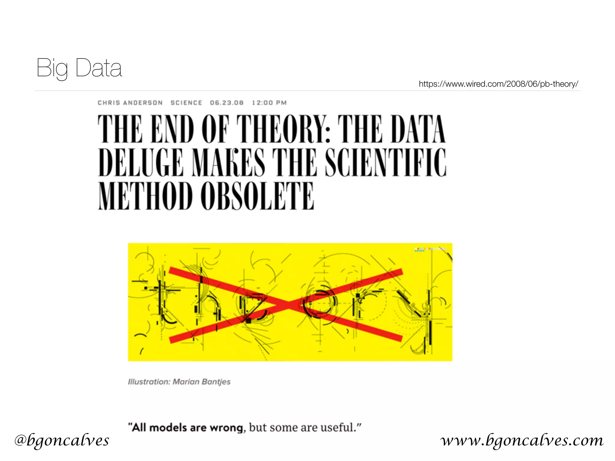
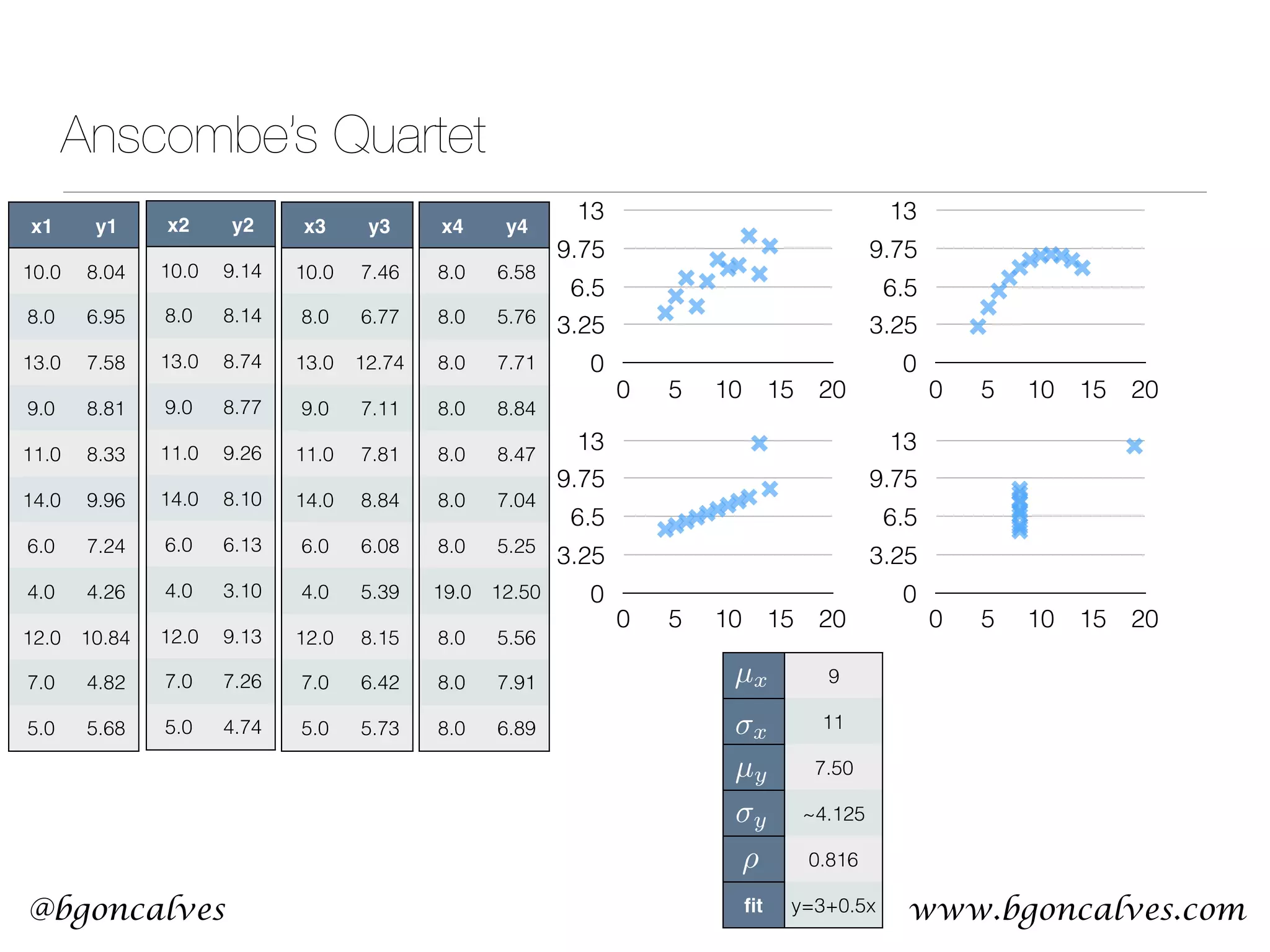
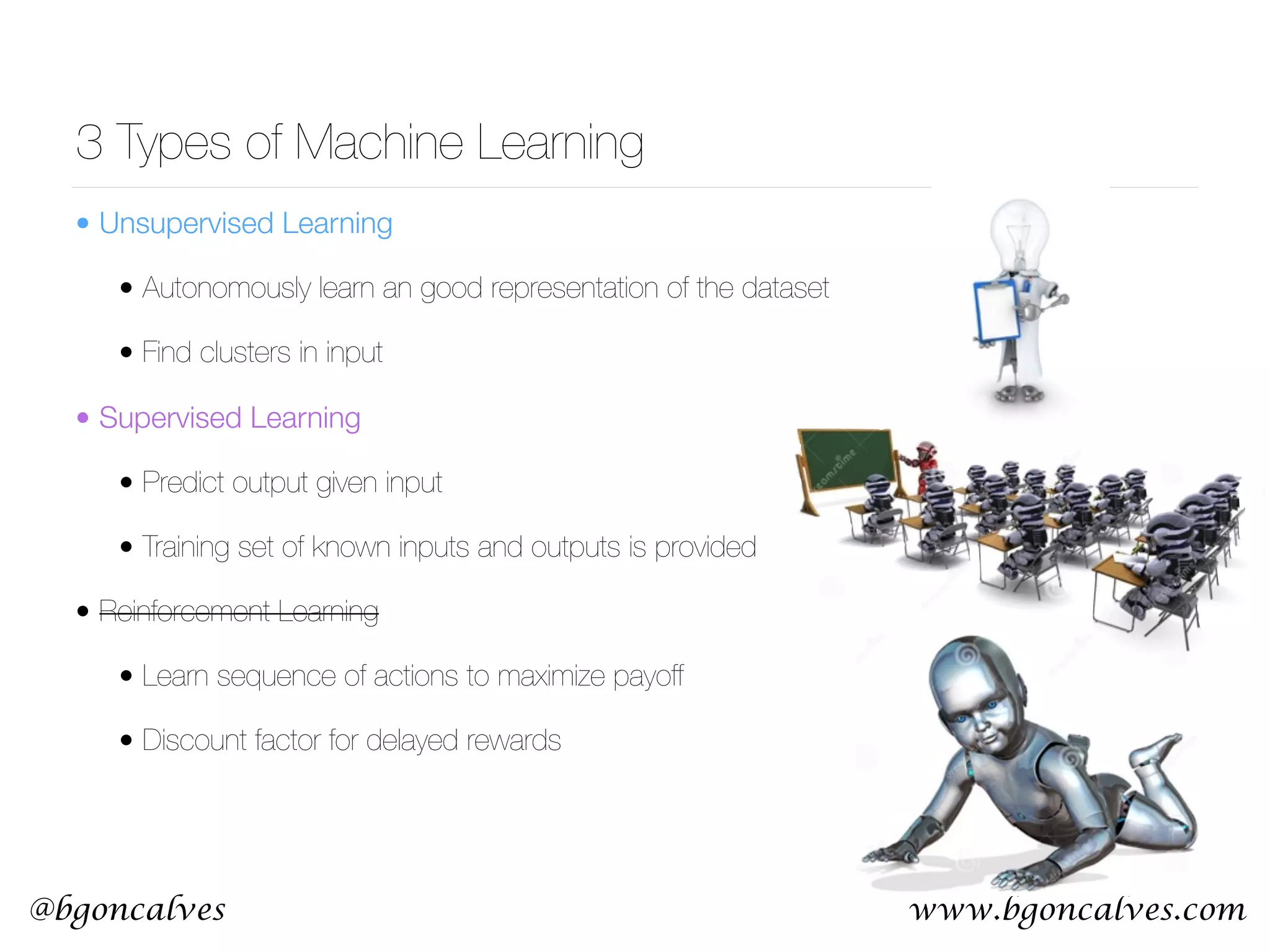
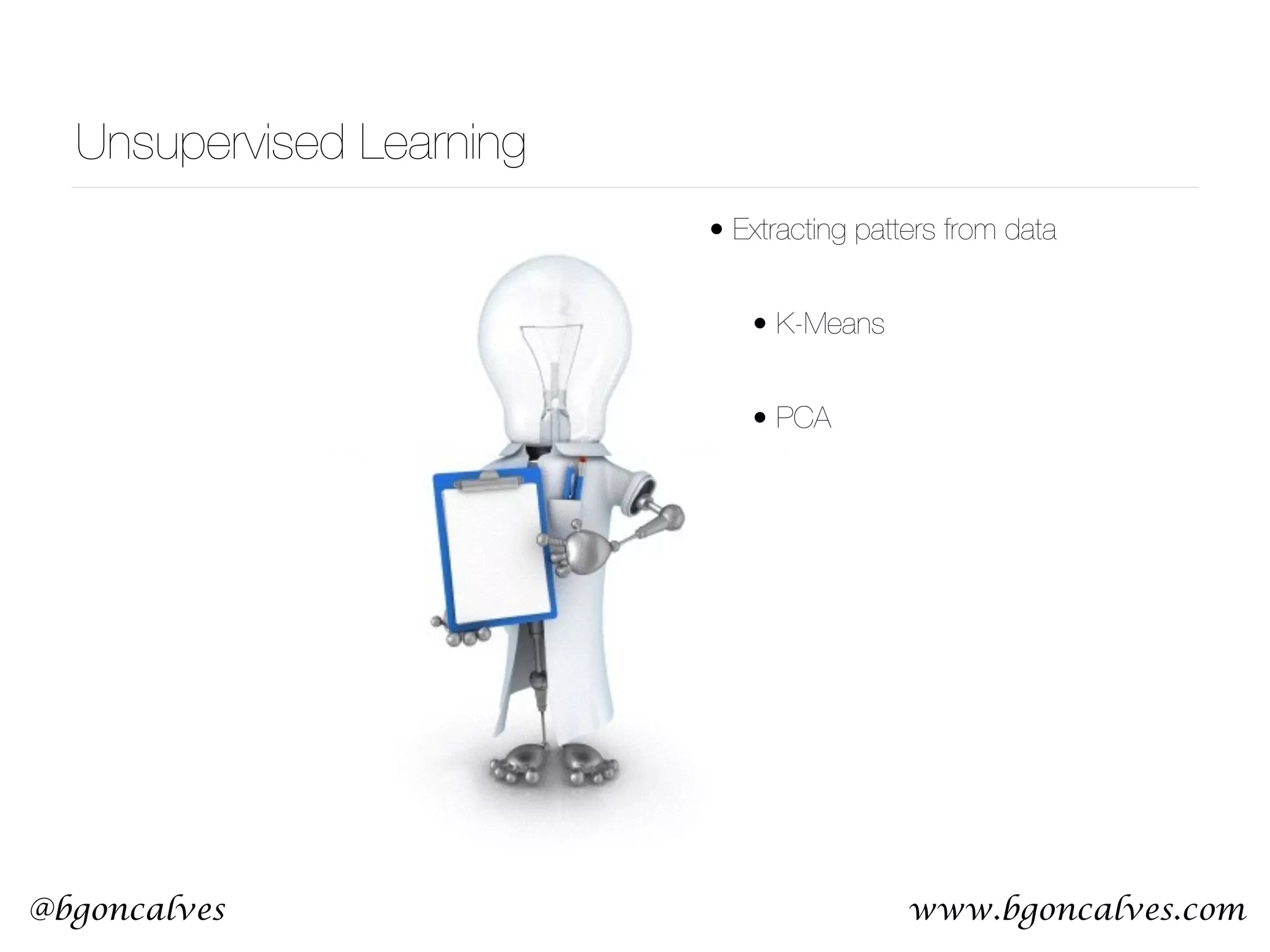
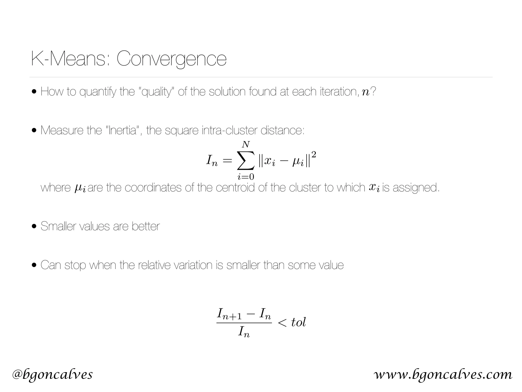
This document serves as a practical introduction to machine learning, covering essential statistical concepts, data analysis techniques, and various machine learning methods including supervised and unsupervised learning. Key topics discussed include the importance of data, statistical measures, clustering algorithms like k-means, and the basics of neural networks along with concepts such as bias-variance tradeoff. Additional emphasis is placed on understanding and minimizing errors in model fitting and the significance of generalization in machine learning.