Downloaded 75 times

![Epoch / Batch / Iteration *One Epoch: One forward pass and one backward pass of all the training examples *Batch Size: The number of training examples in one forward/backward pass. The higher the batch size, the more memory space you'll need. Minibatch: Take a small number of examples at a time, ranging from 1 to a few hundred, during one iteration. *Number of Iterations: Number of passes, each pass using [batch size] number of examples. To be clear, one pass = one forward pass + one backward pass. *Quote from http://stackoverflow.com/questions/4752626/epoch-vs-iteration- when-training-neural-networks/31842945#31842945](https://image.slidesharecdn.com/dl101-chap5jasontfrankw2016-170328160123/75/Deep-Learning-Introduction-Chapter-5-Machine-Learning-Basics-14-2048.jpg)

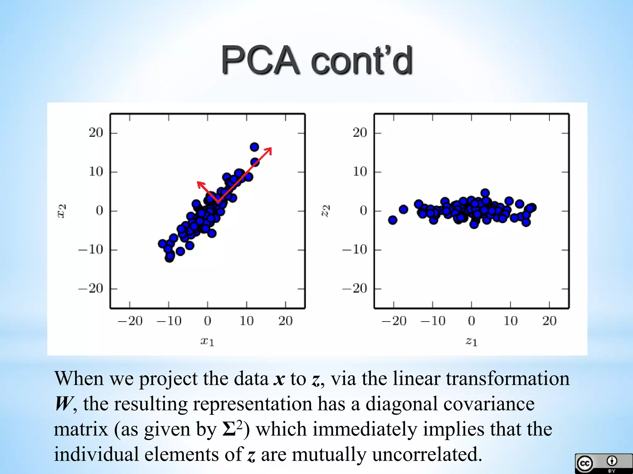
![PCA cont’d Find where Var[z] is diagonal given](https://image.slidesharecdn.com/dl101-chap5jasontfrankw2016-170328160123/75/Deep-Learning-Introduction-Chapter-5-Machine-Learning-Basics-47-2048.jpg)

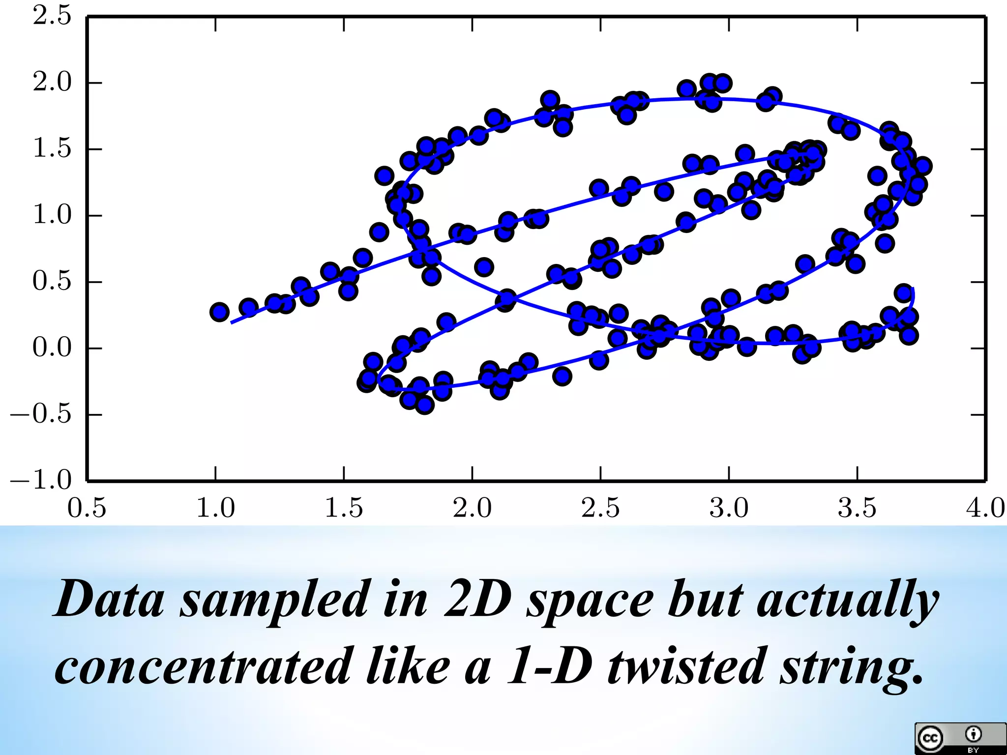
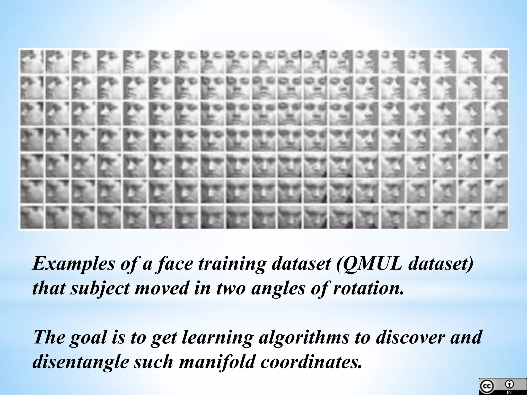
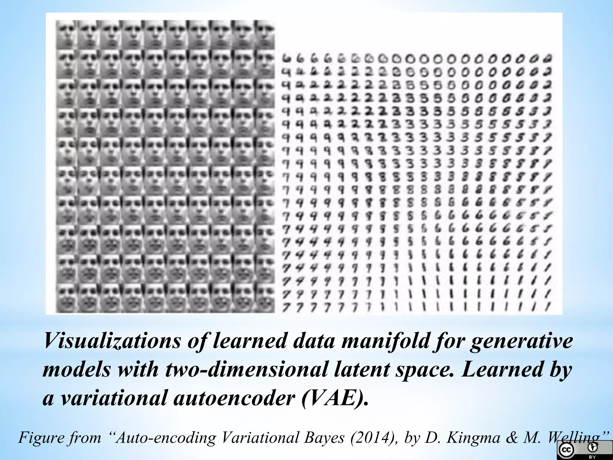


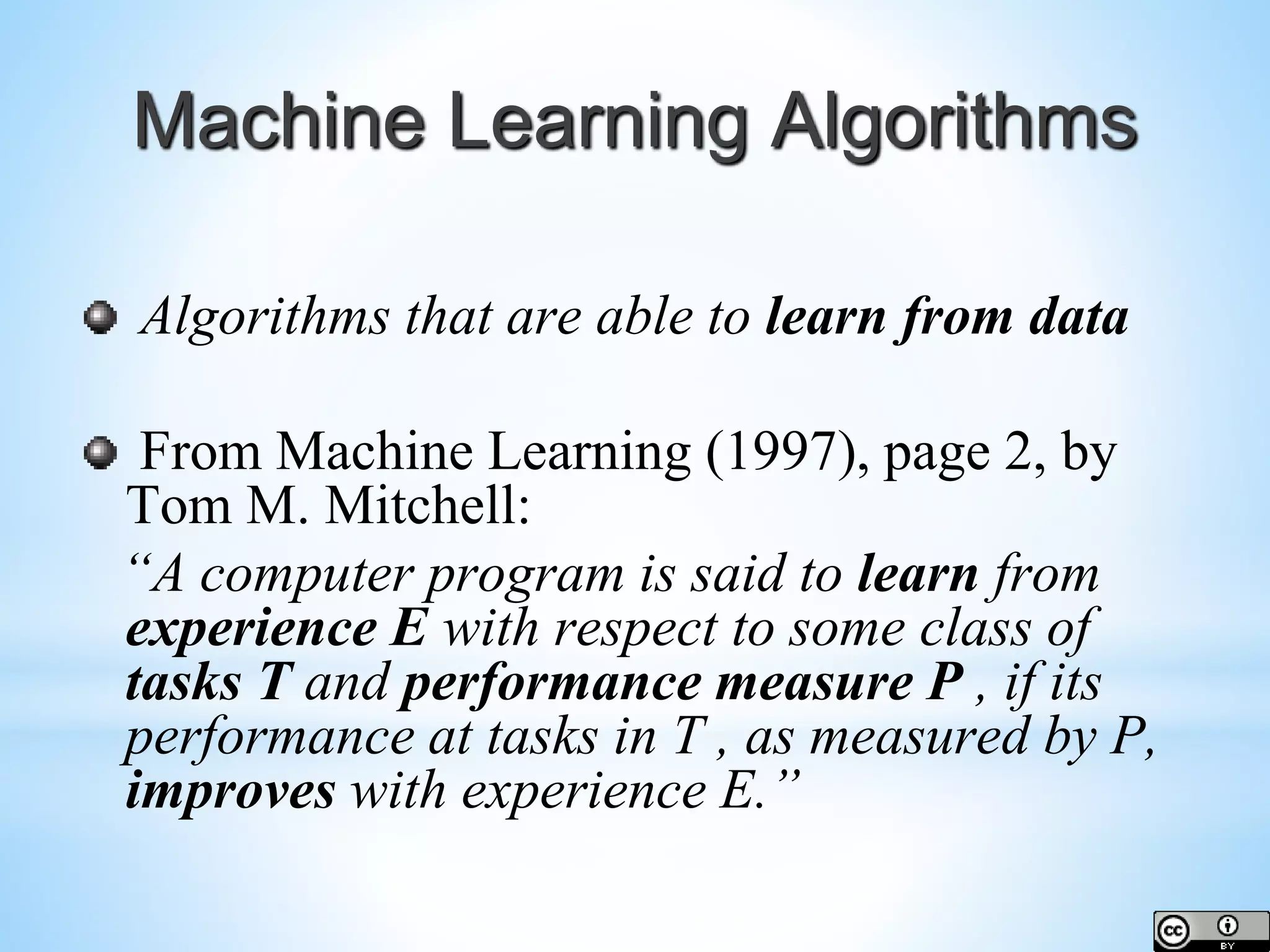
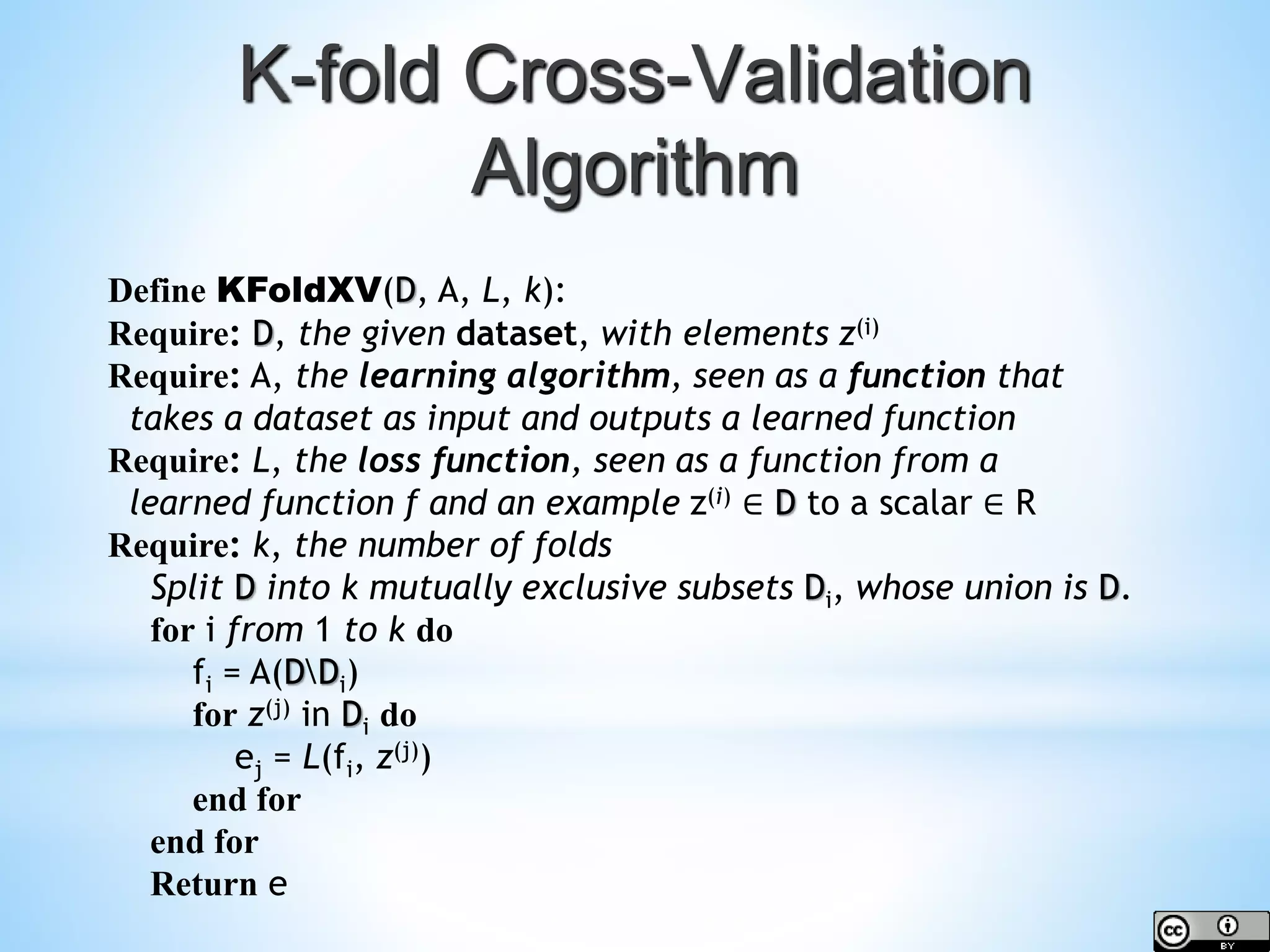
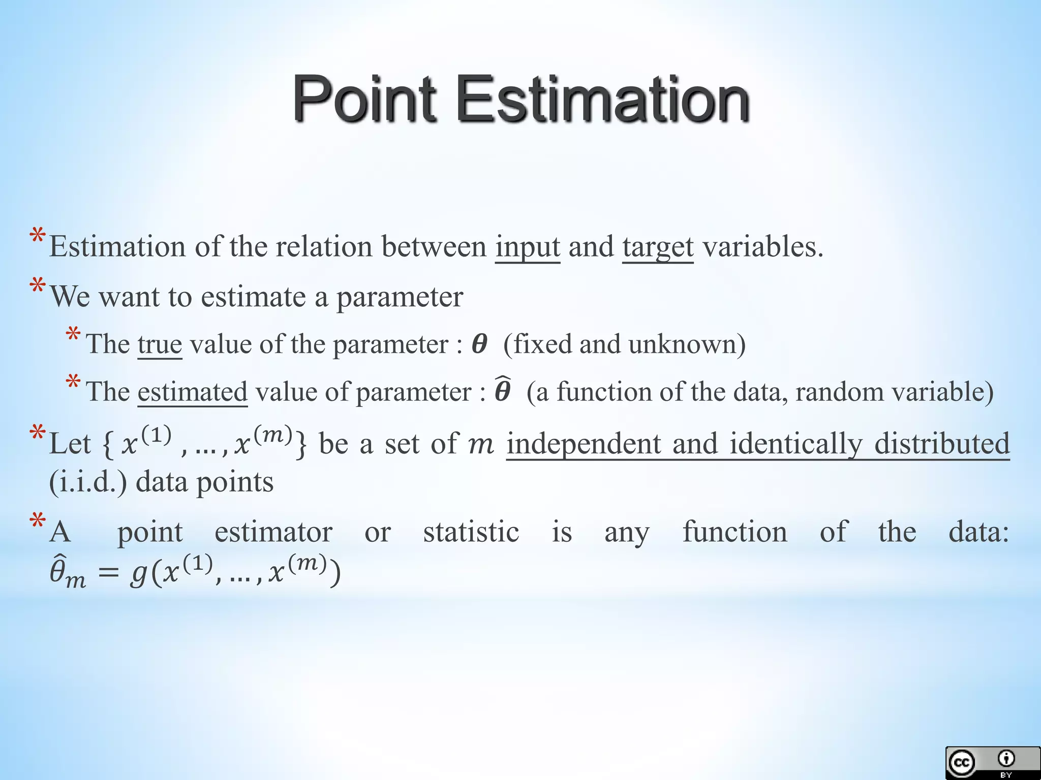
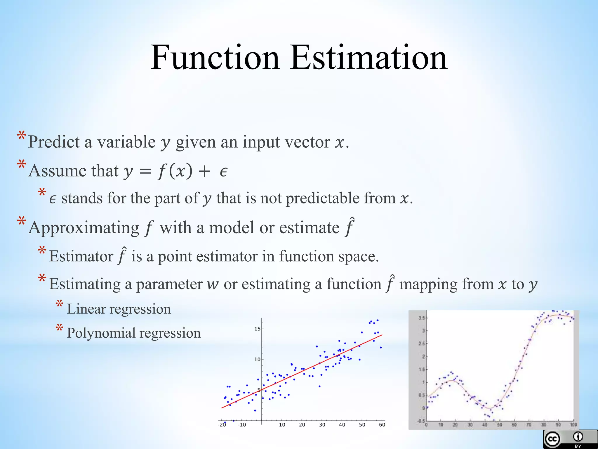
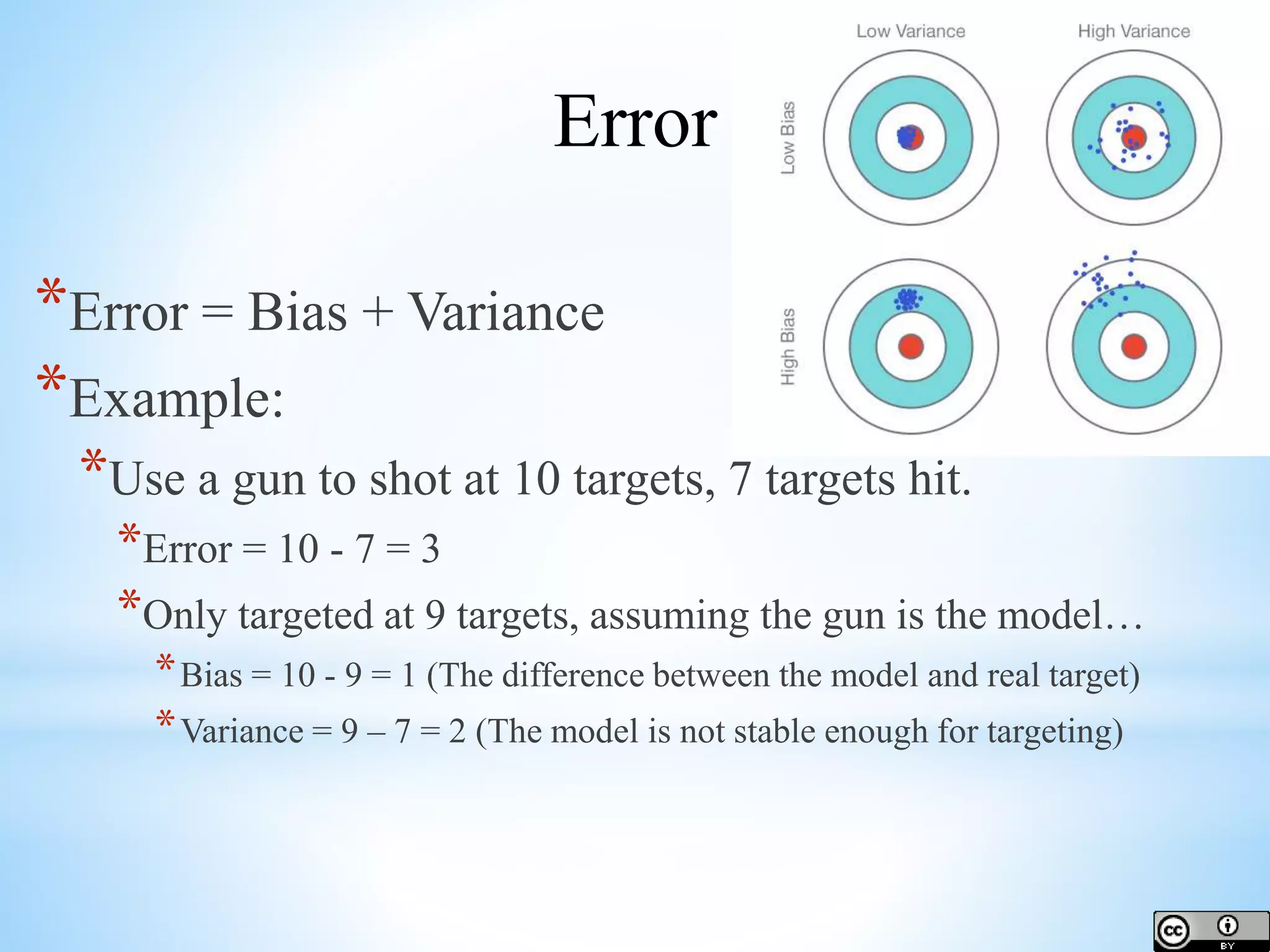
The document provides an overview of deep learning concepts including activation functions, machine learning algorithms, learning paradigms, and key techniques such as stochastic gradient descent and k-fold cross-validation. It discusses challenges in model performance such as overfitting and underfitting, and introduces essential statistical methods like maximum likelihood estimation and principal component analysis. The document also emphasizes the significance of deep learning in addressing the curse of dimensionality and manifold learning in high-dimensional data representation.