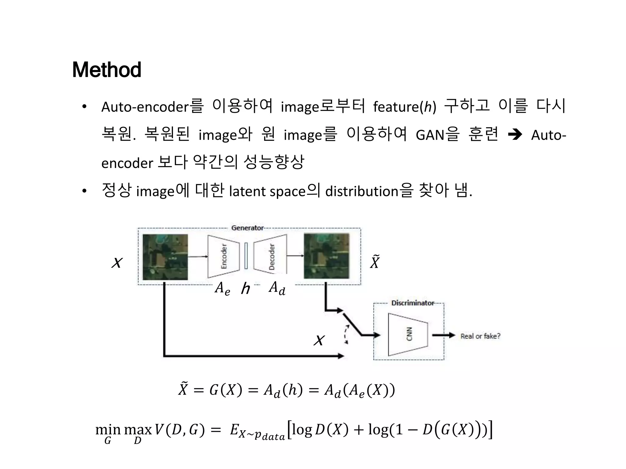
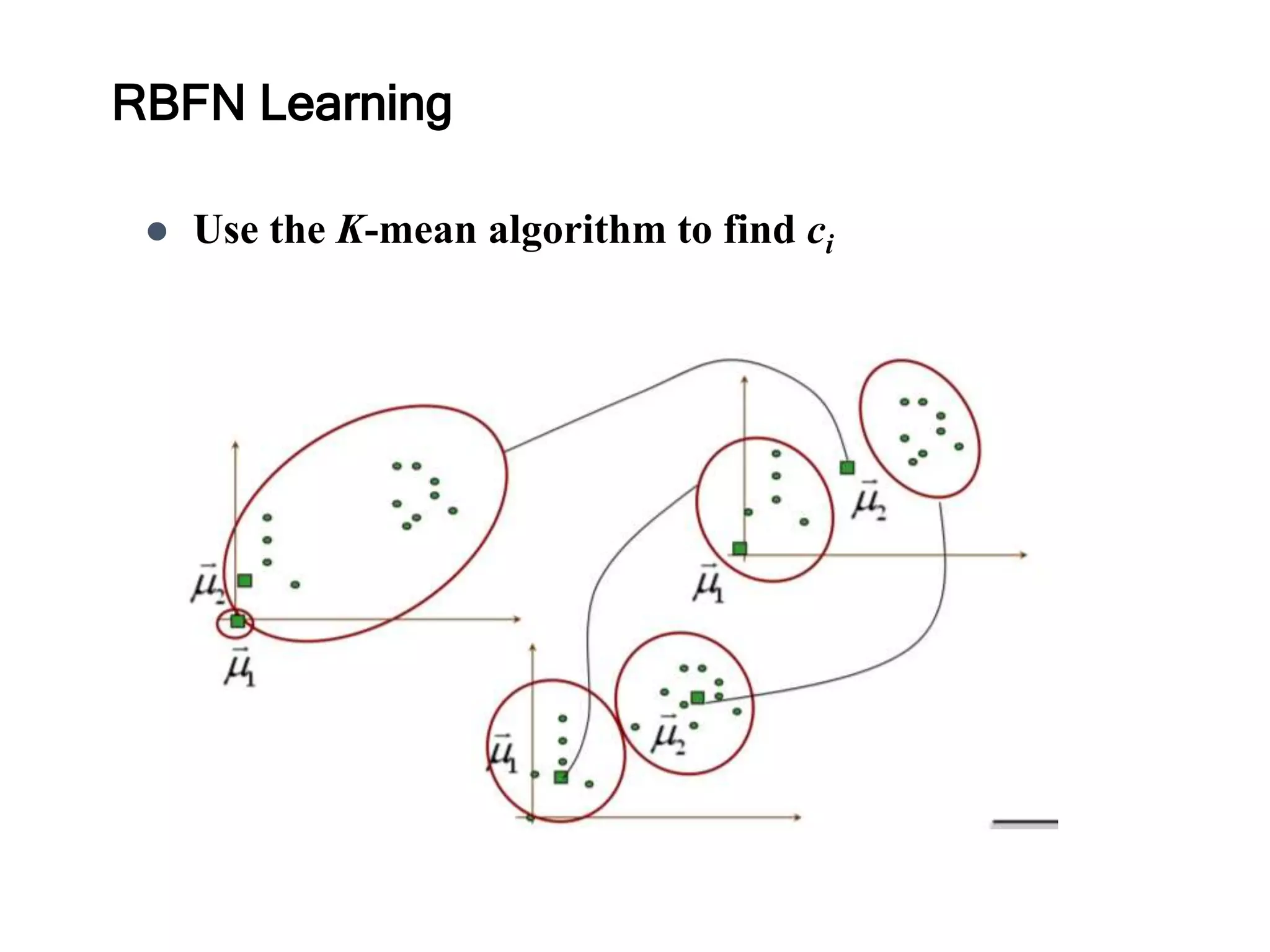
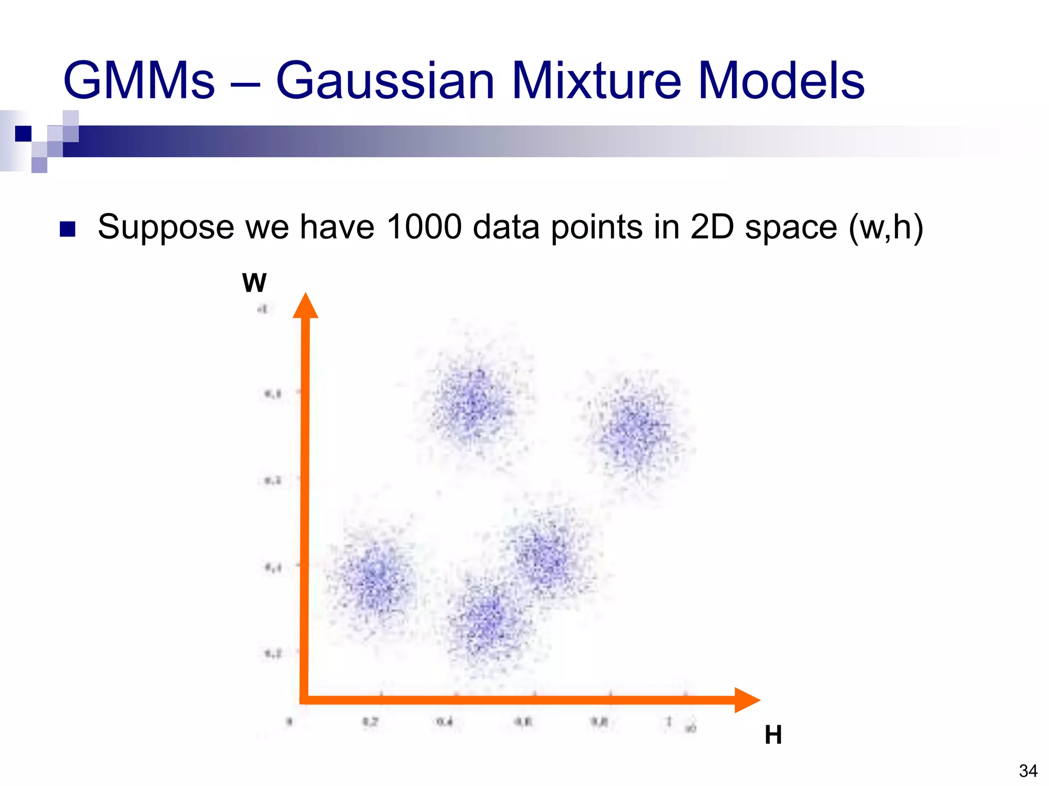
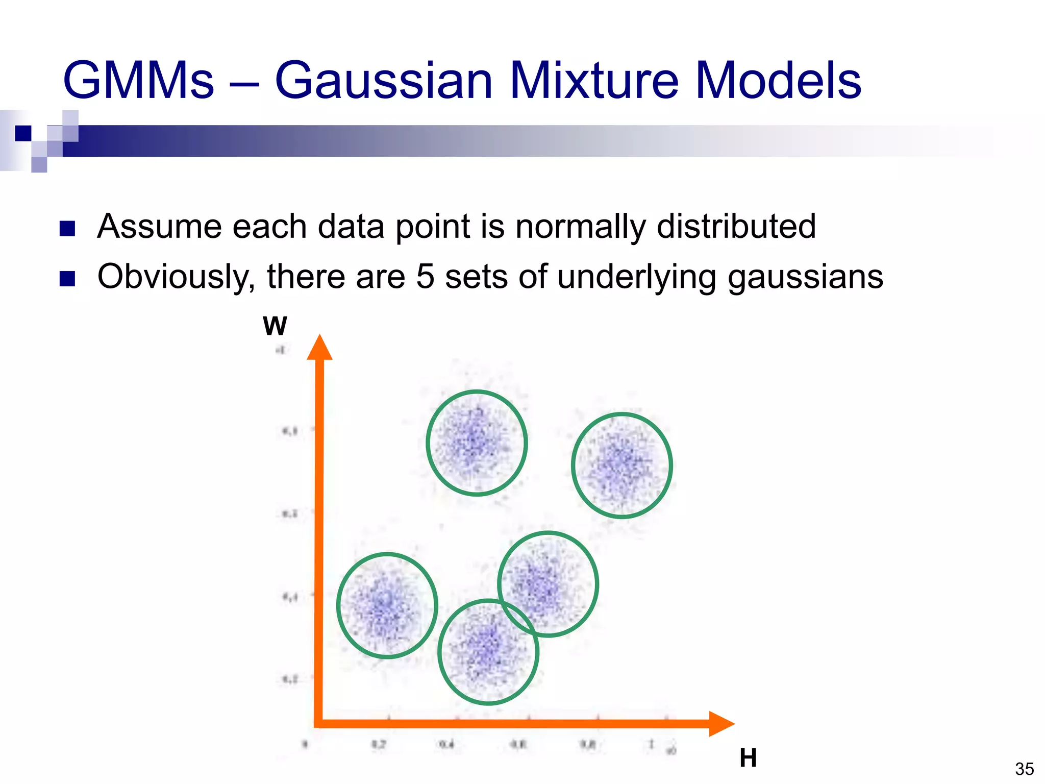
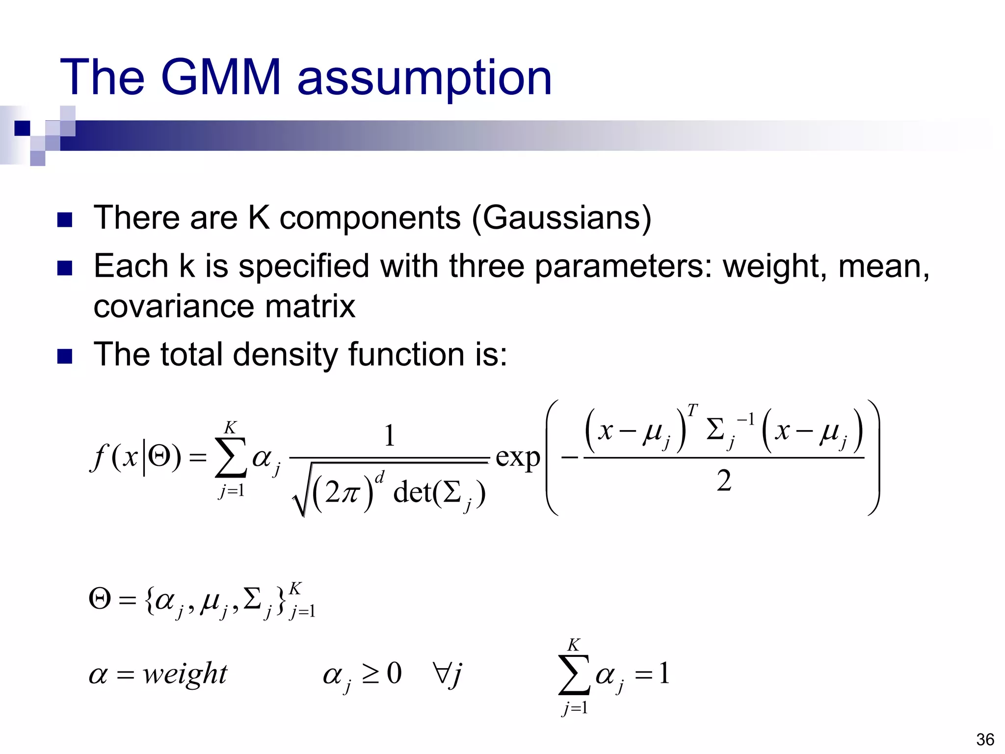
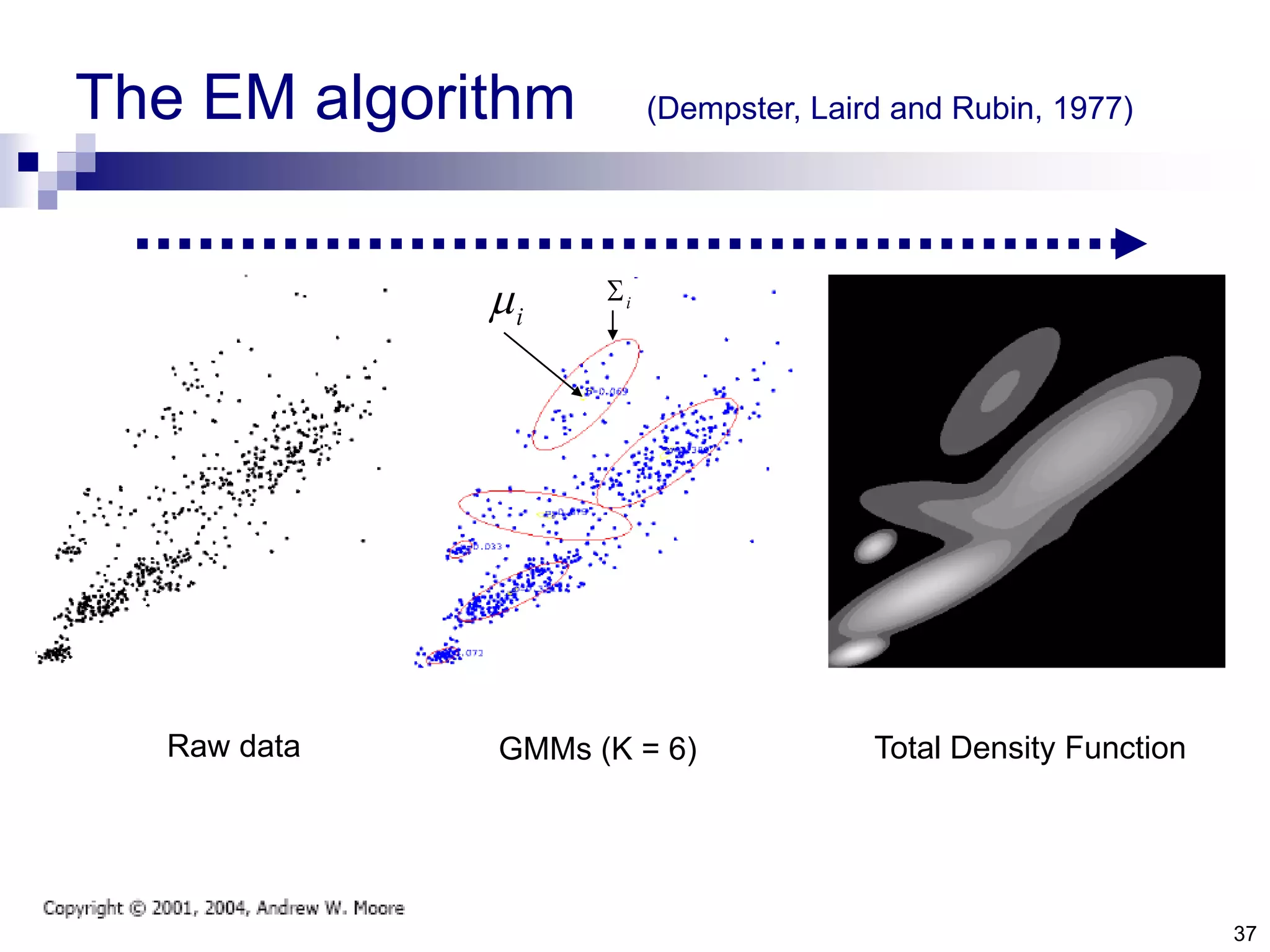
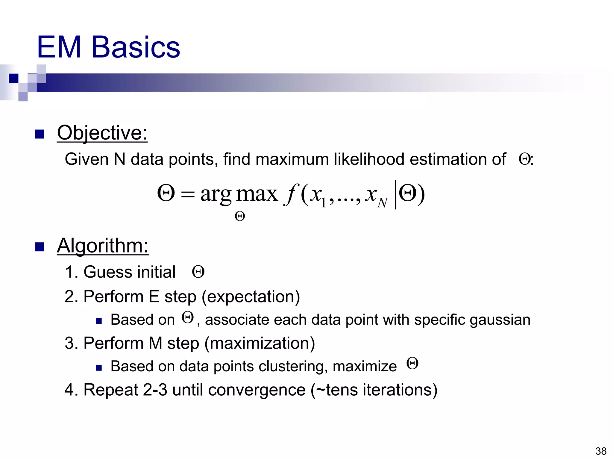
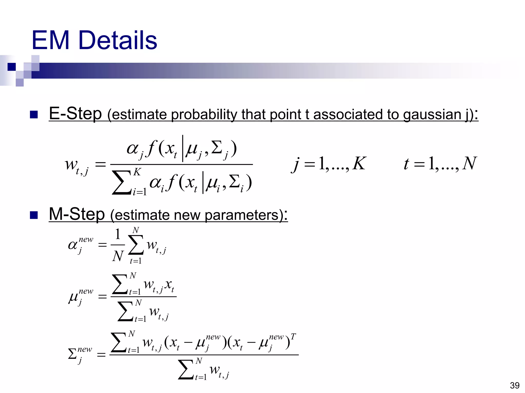
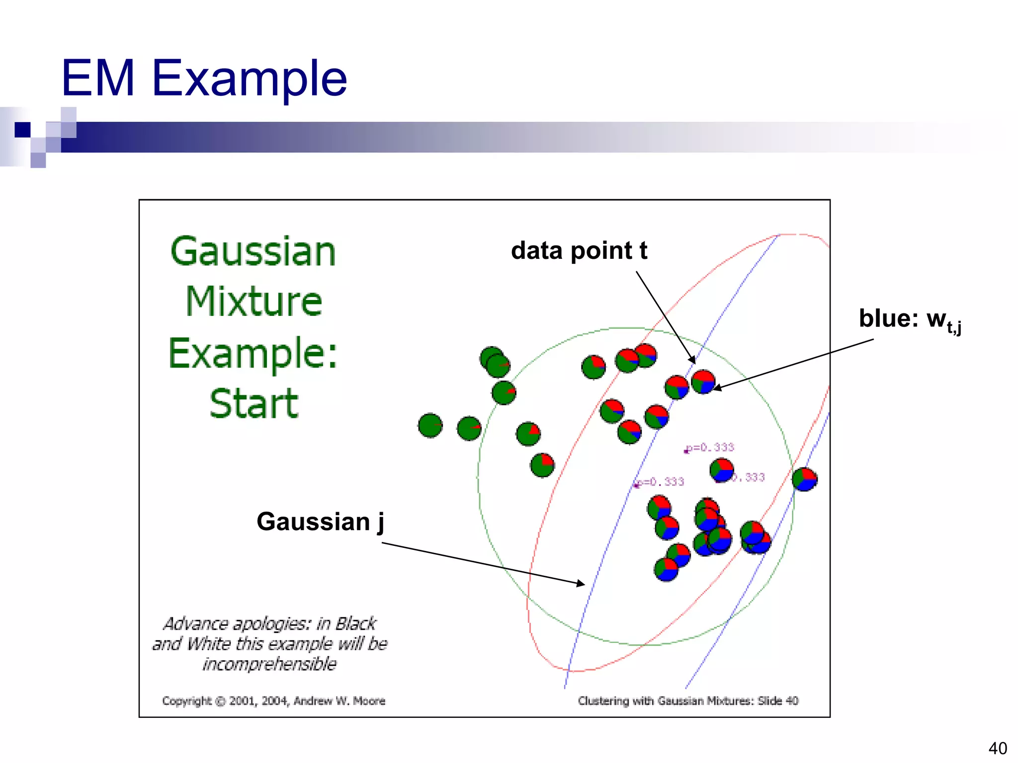
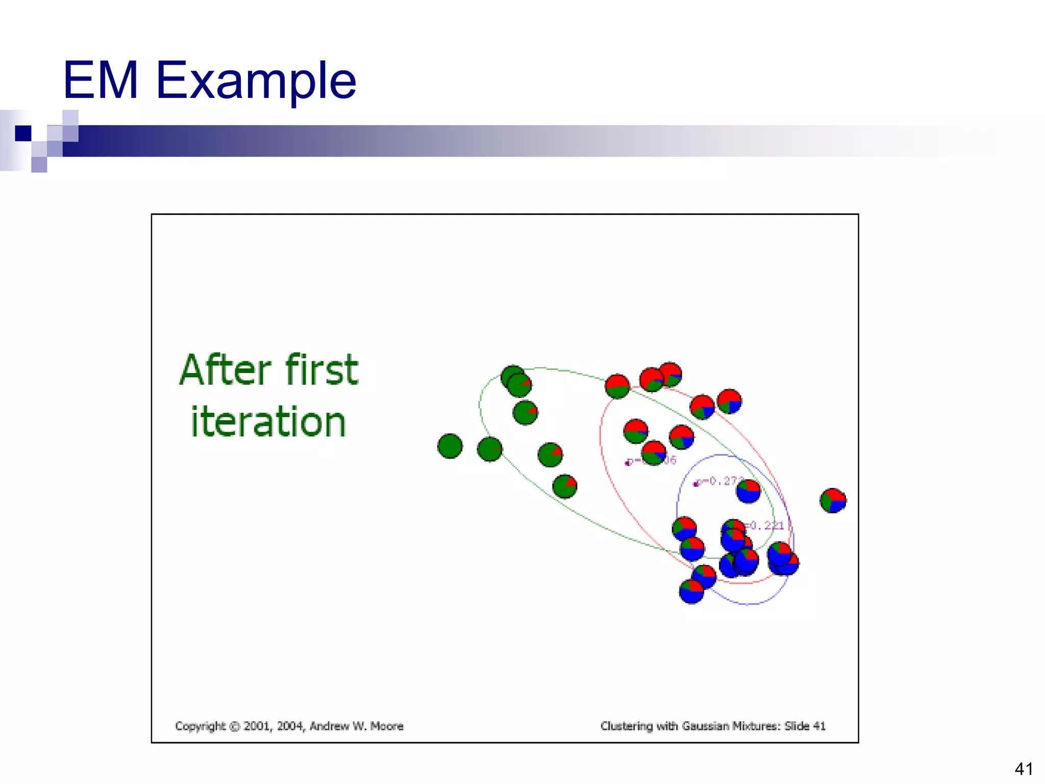
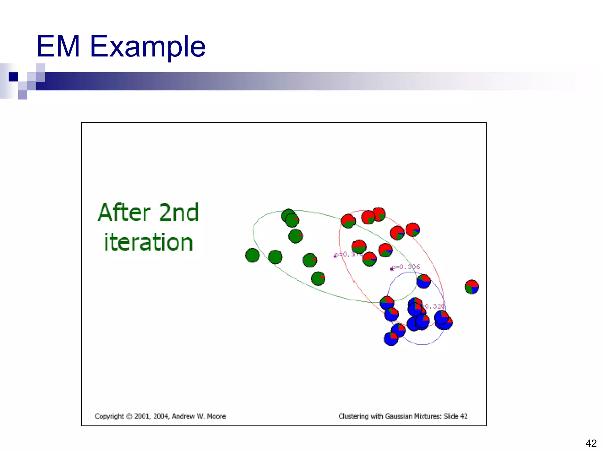
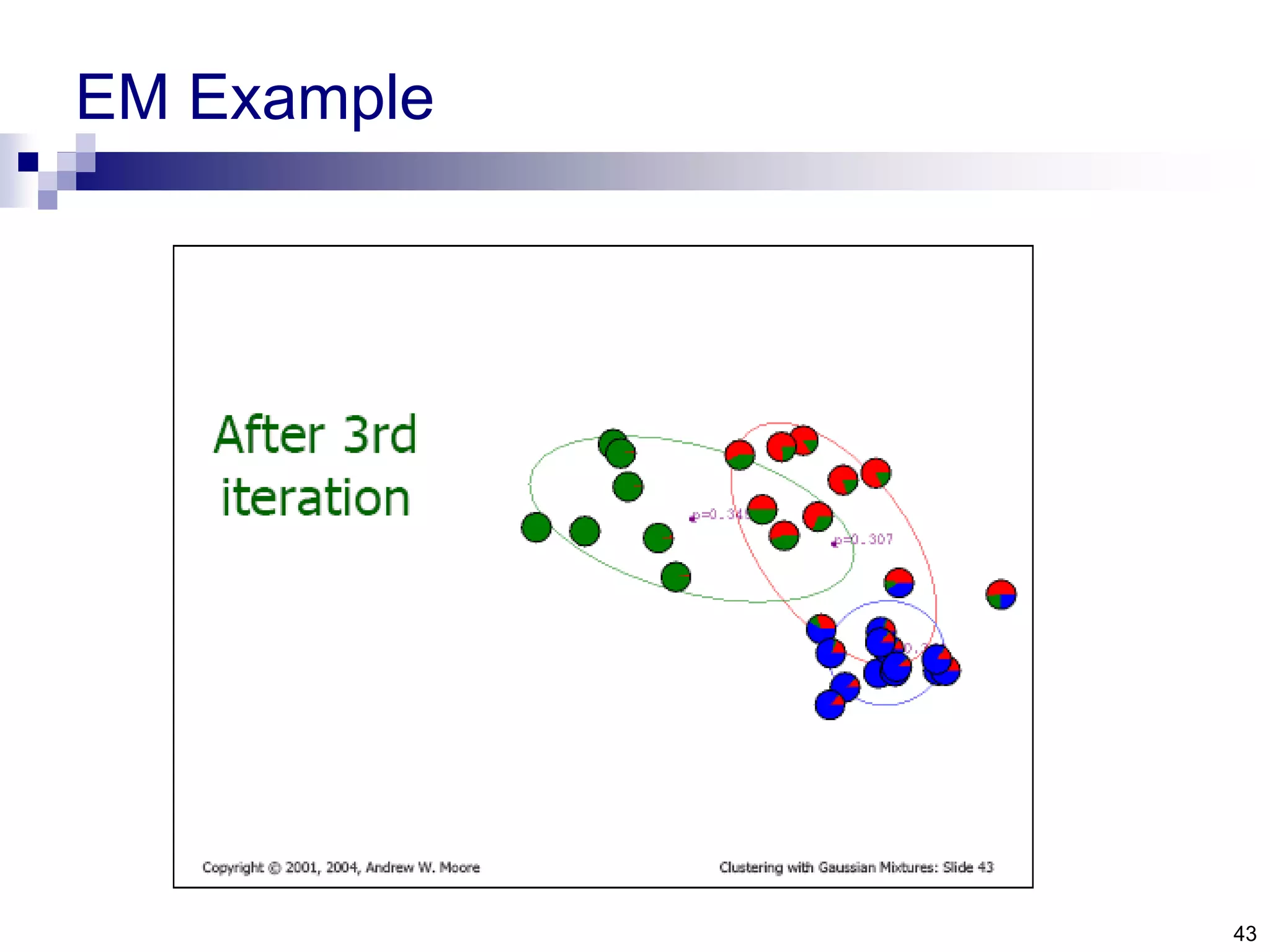
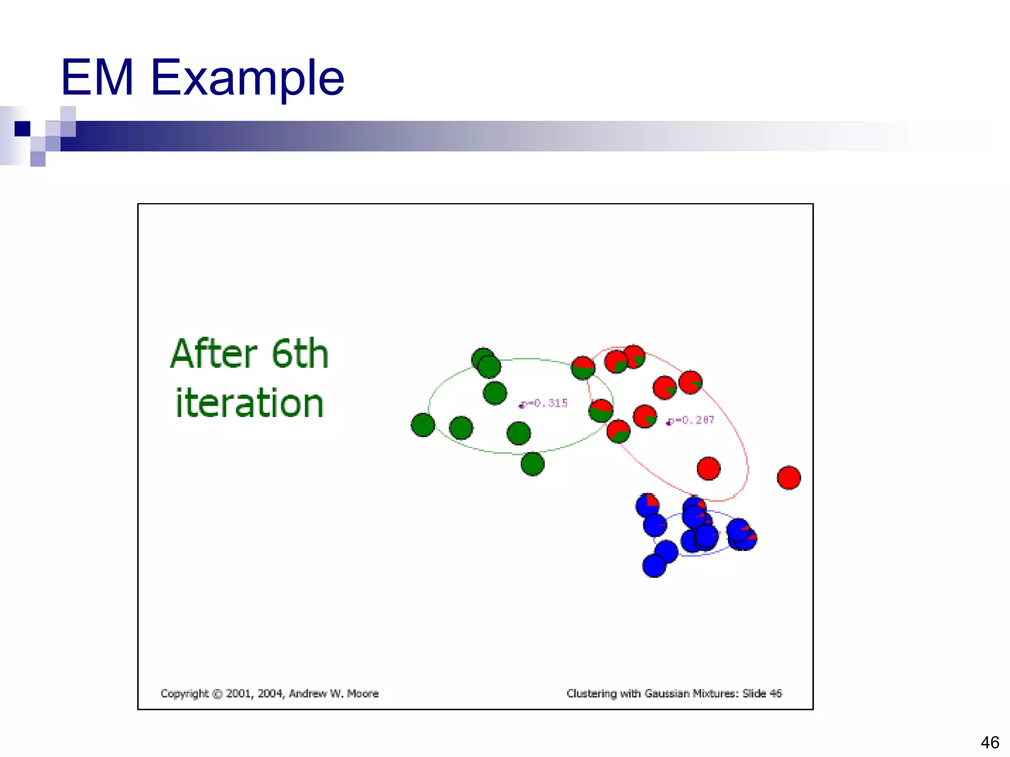
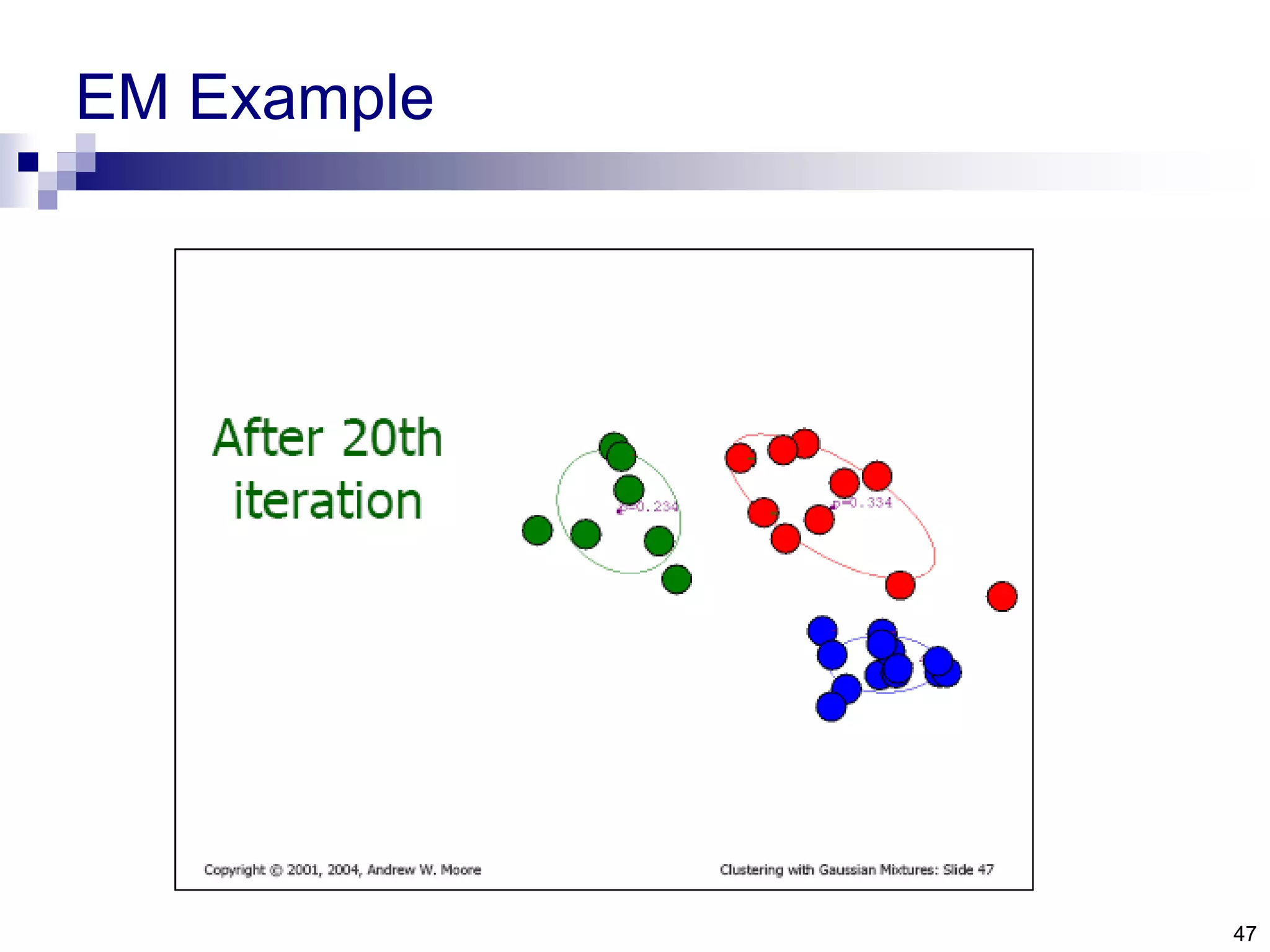
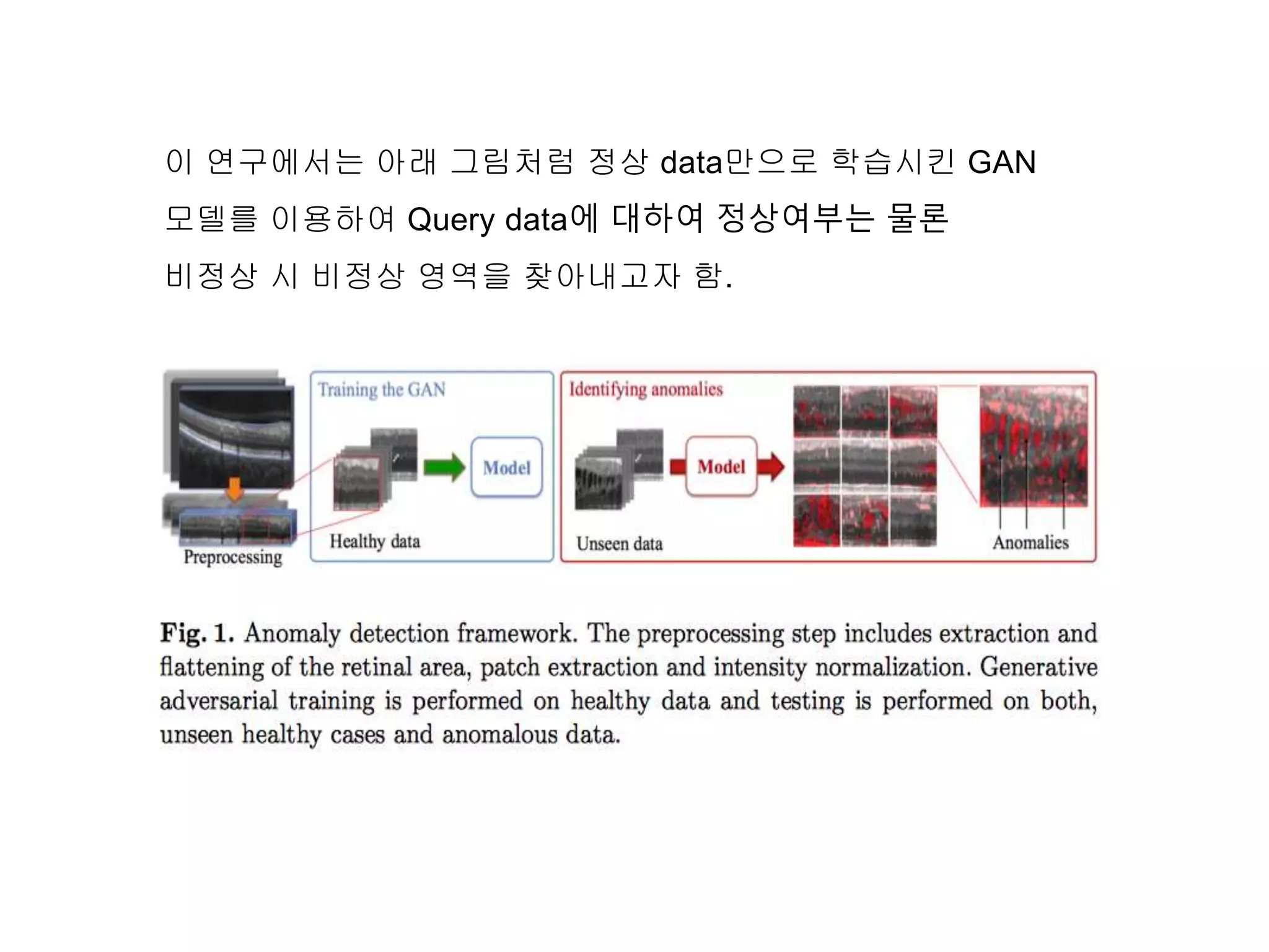
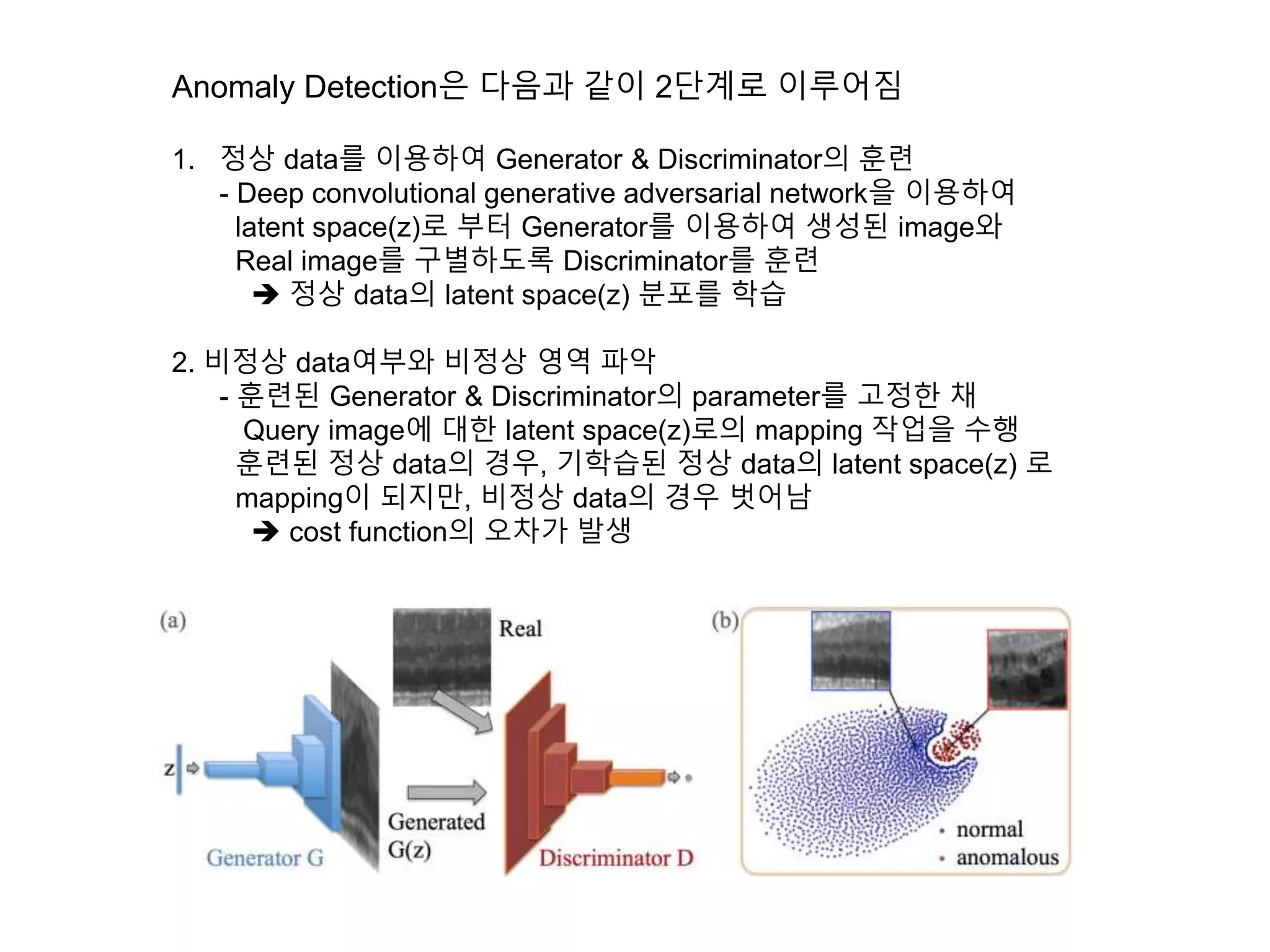
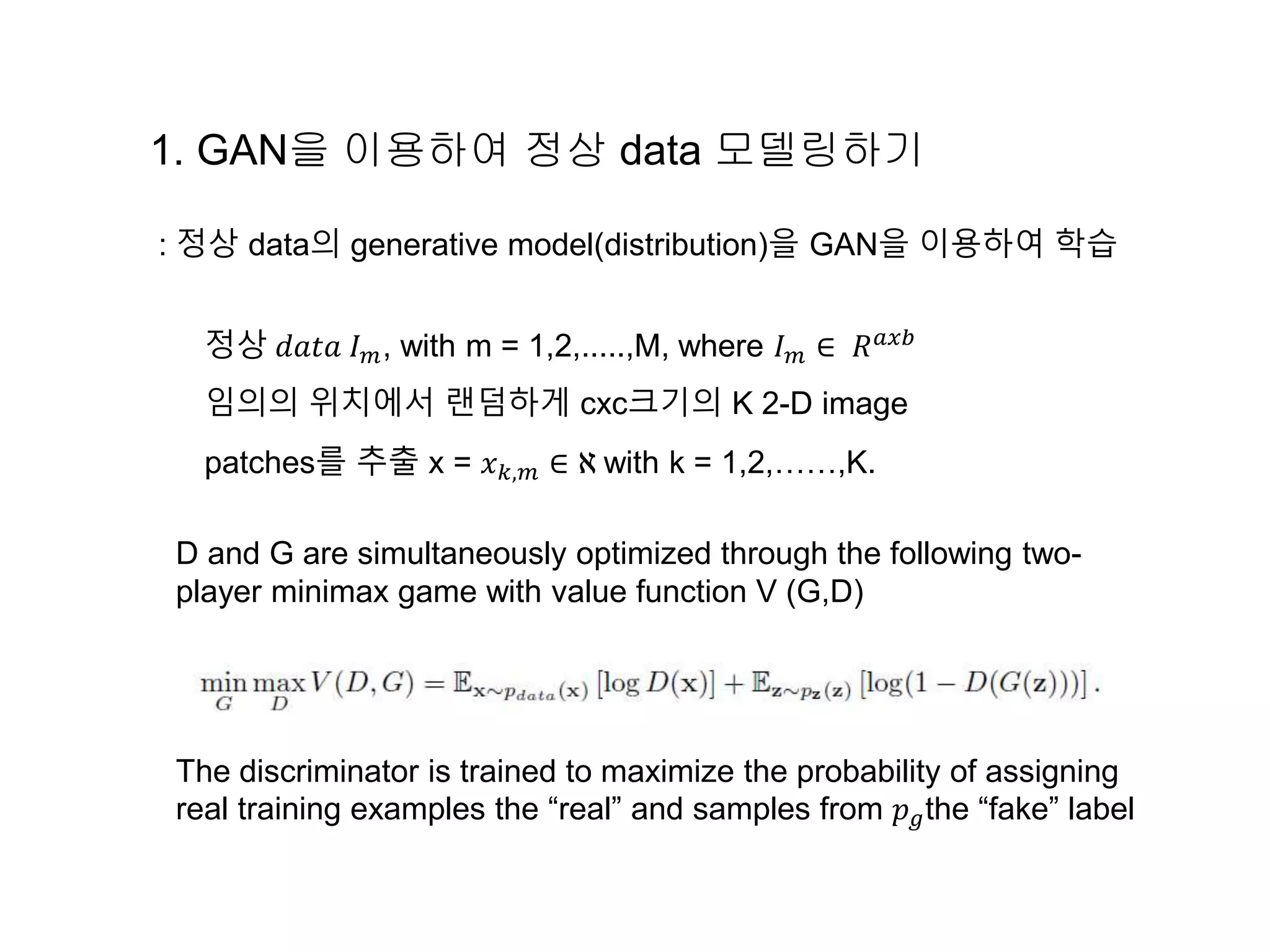
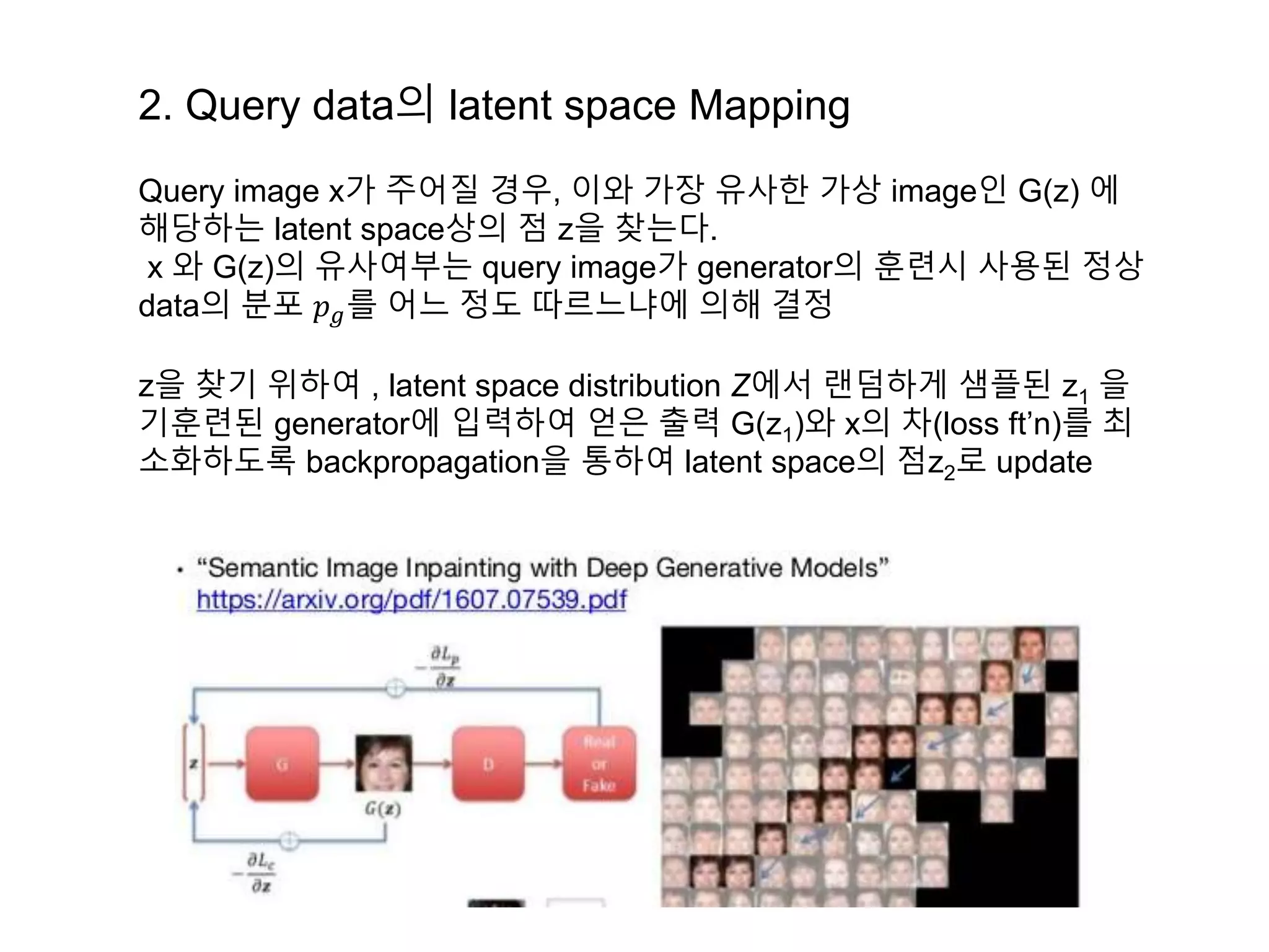
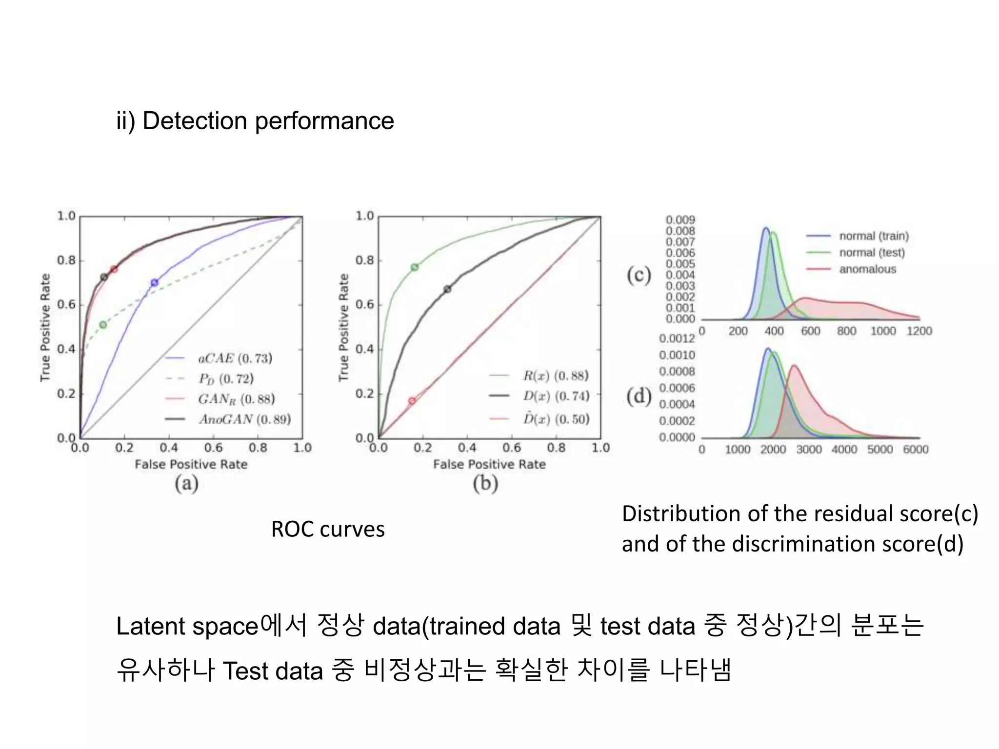
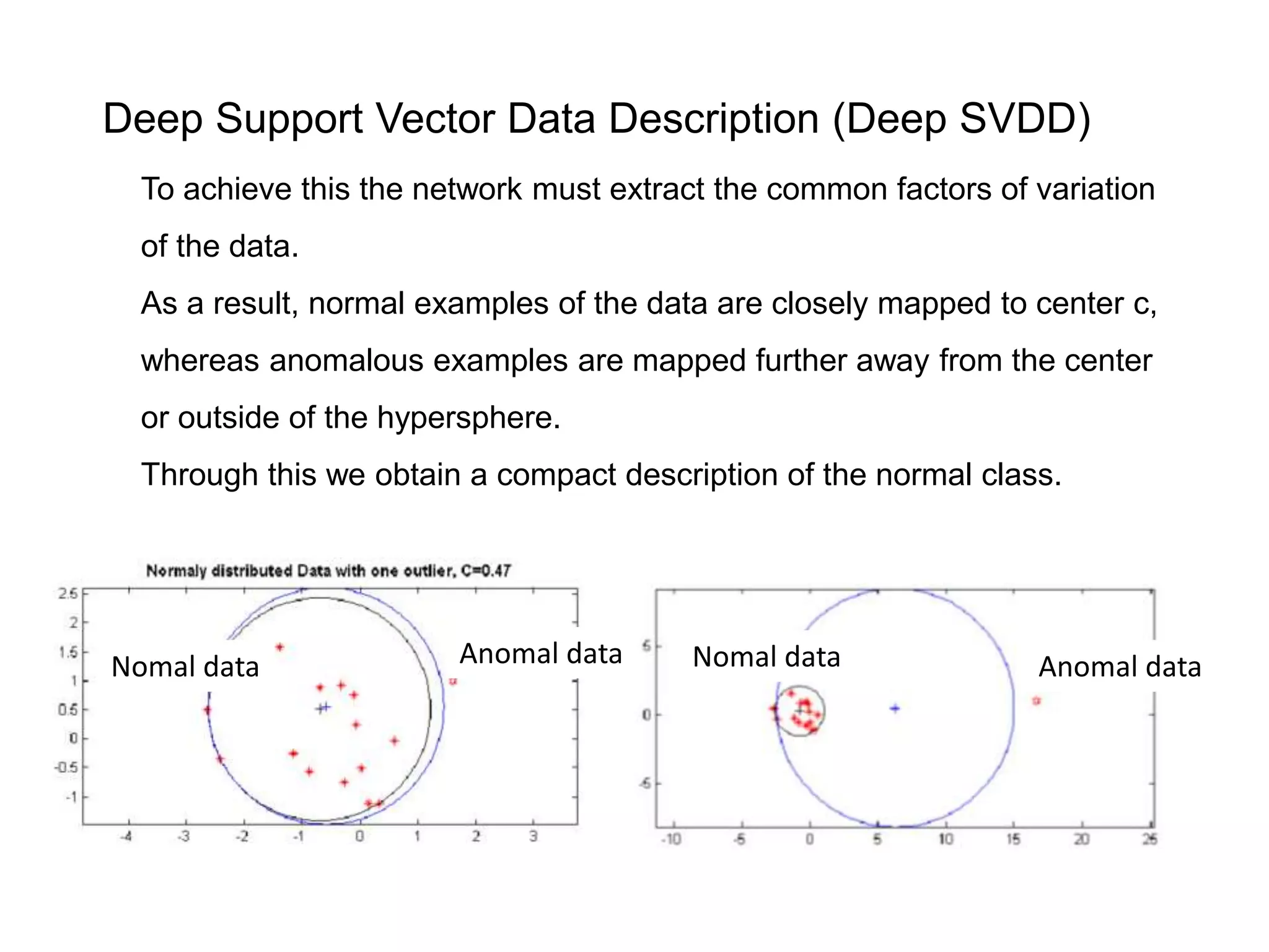
The document discusses anomaly detection techniques using deep one-class classifiers and generative adversarial networks (GANs). It proposes using an autoencoder to extract features from normal images, training a GAN on those features to model the distribution, and using a one-class support vector machine (SVM) to determine if new images are within the normal distribution. The method detects and localizes anomalies by generating a binary mask for abnormal regions. It also discusses Gaussian mixture models and the expectation-maximization algorithm for modeling multiple distributions in data.


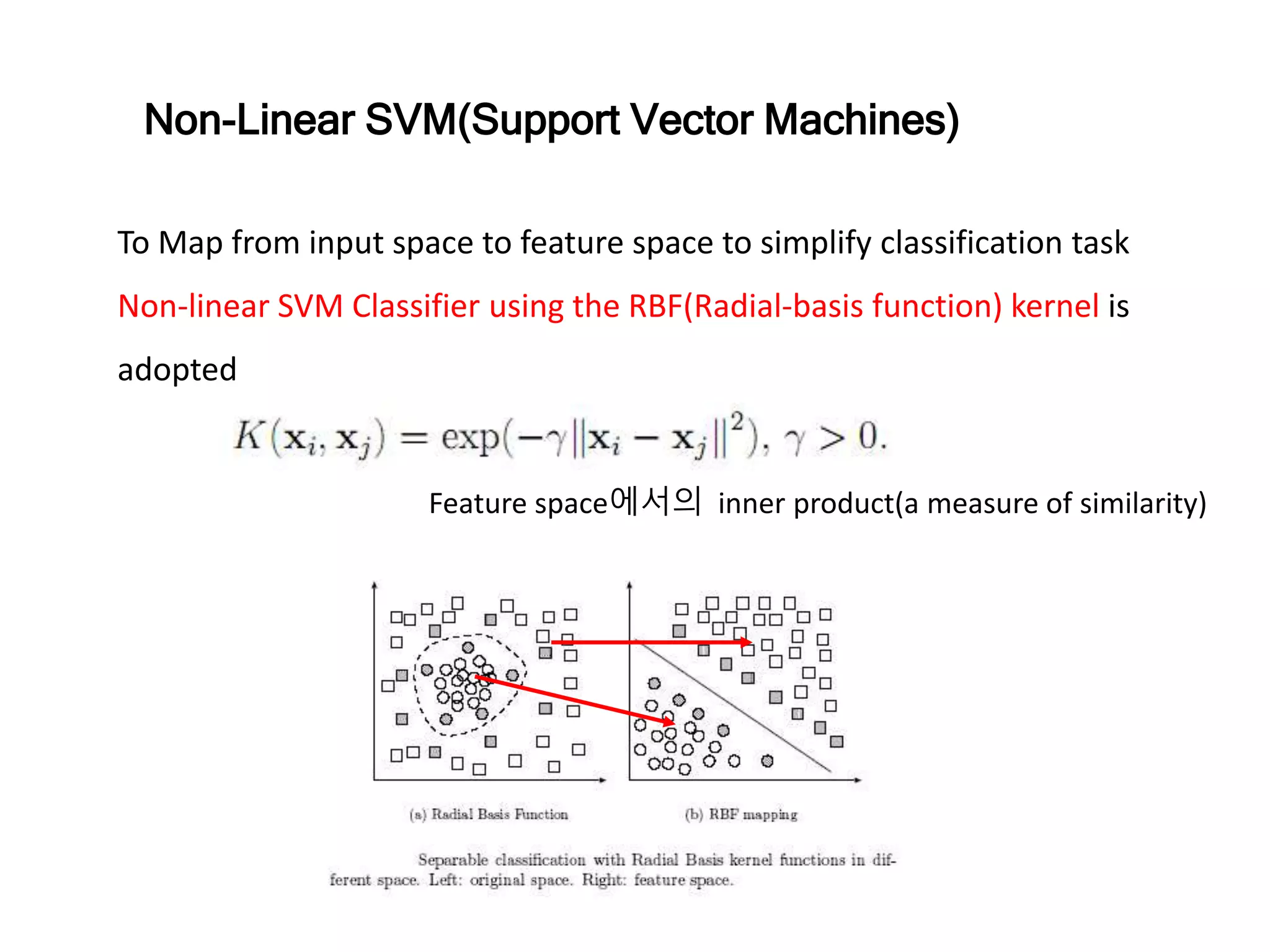
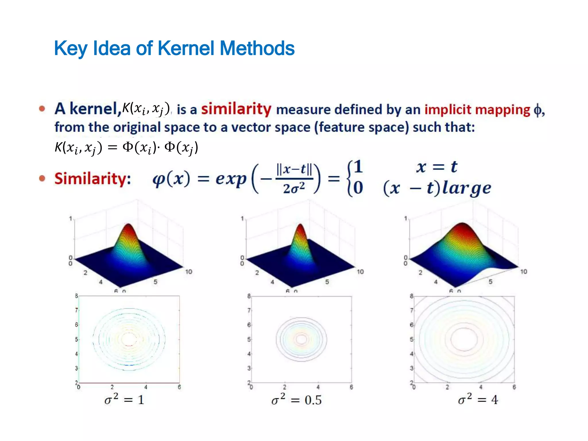
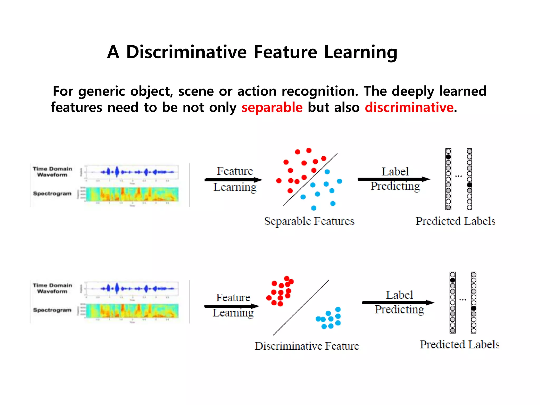
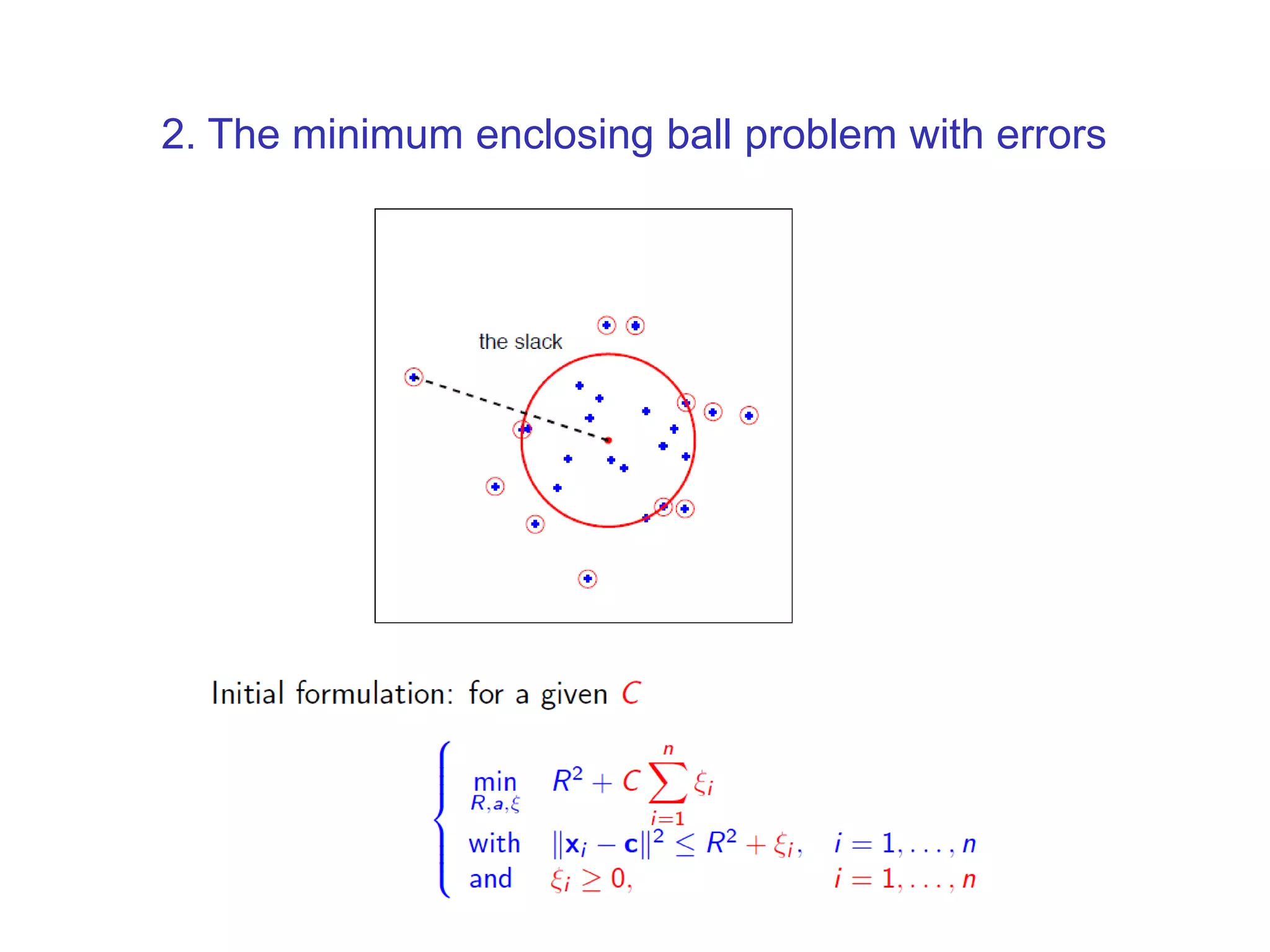
![Normal Condition : Cluster bound : exp{− [ 𝑥1−𝑐1 2+ 𝑥2−𝑐2 2] 2𝜎2 } ≥ {0<Threshold<<1} 𝑥1 − 𝑐1 2 + 𝑥2 − 𝑐2 2 ≤ r2 𝐾1 + 𝐾2 ≤ r2 x1 x2 .(c1,c2) r K1 K2 r2 r2 Key Idea of Kernel Methods](https://image.slidesharecdn.com/anomalydetectionusingdeeponeclassclassifier-190309014237/75/Anomaly-detection-using-deep-one-class-classifier-13-2048.jpg)


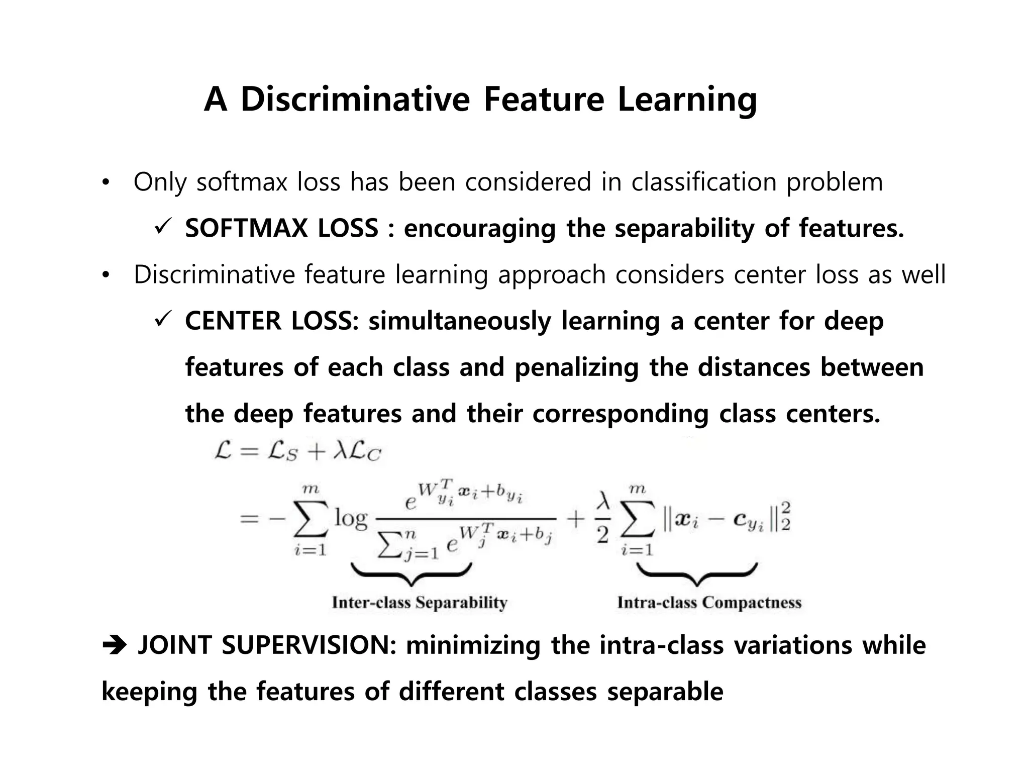
![1. The minimum enclosing ball problem [Tax and Duin, 2004] centerRadius, R](https://image.slidesharecdn.com/anomalydetectionusingdeeponeclassclassifier-190309014237/75/Anomaly-detection-using-deep-one-class-classifier-69-2048.jpg)

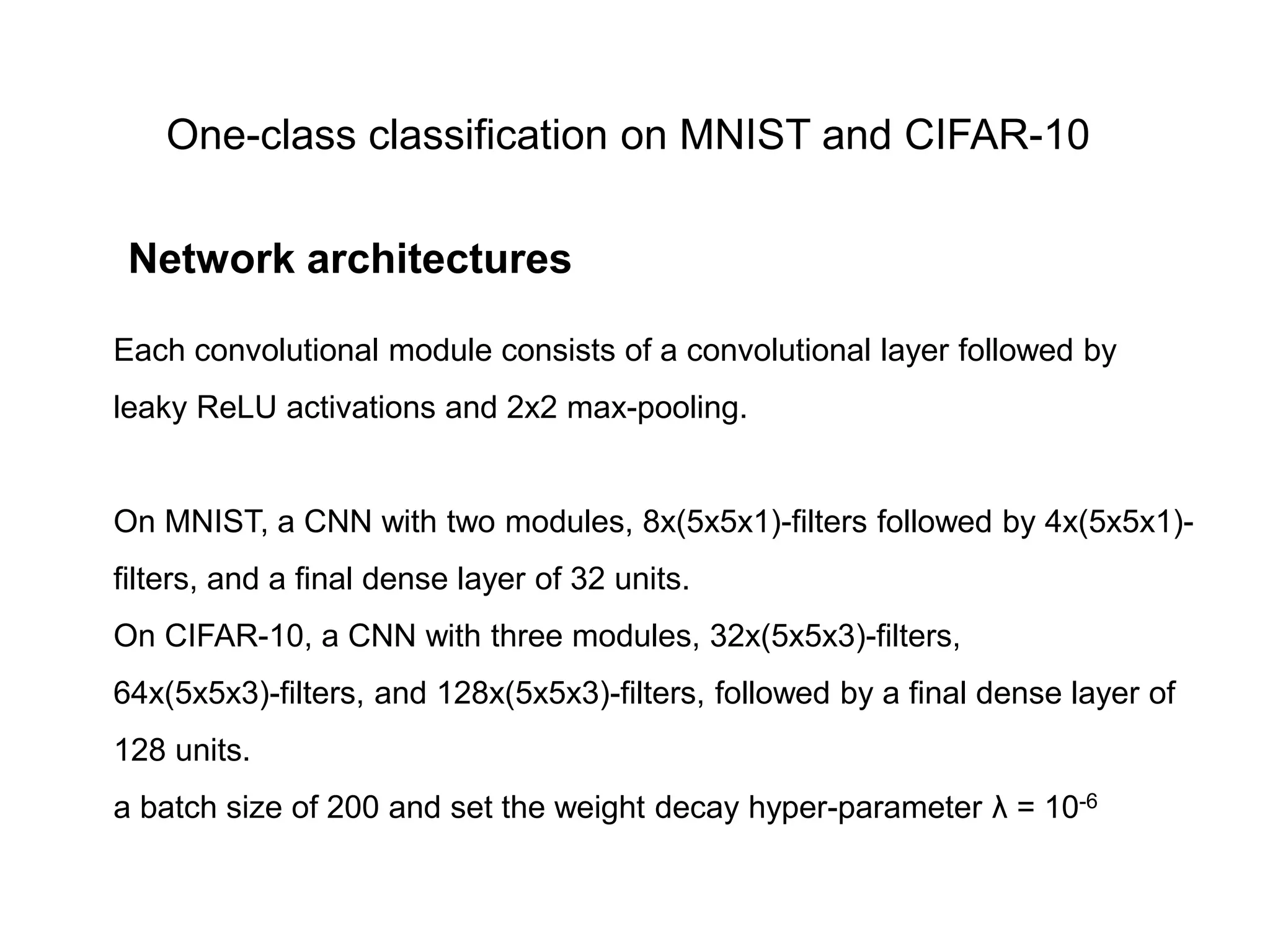
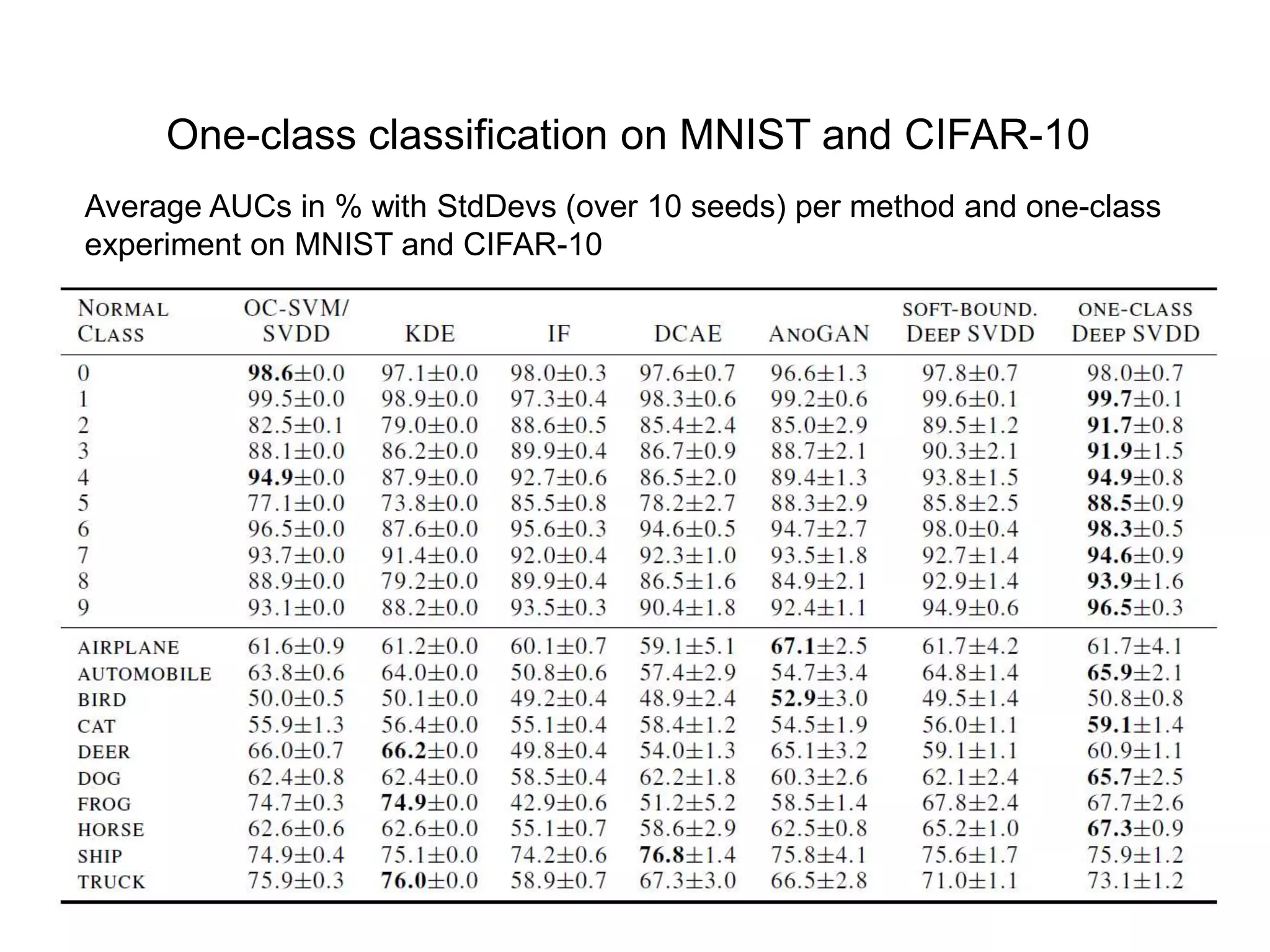
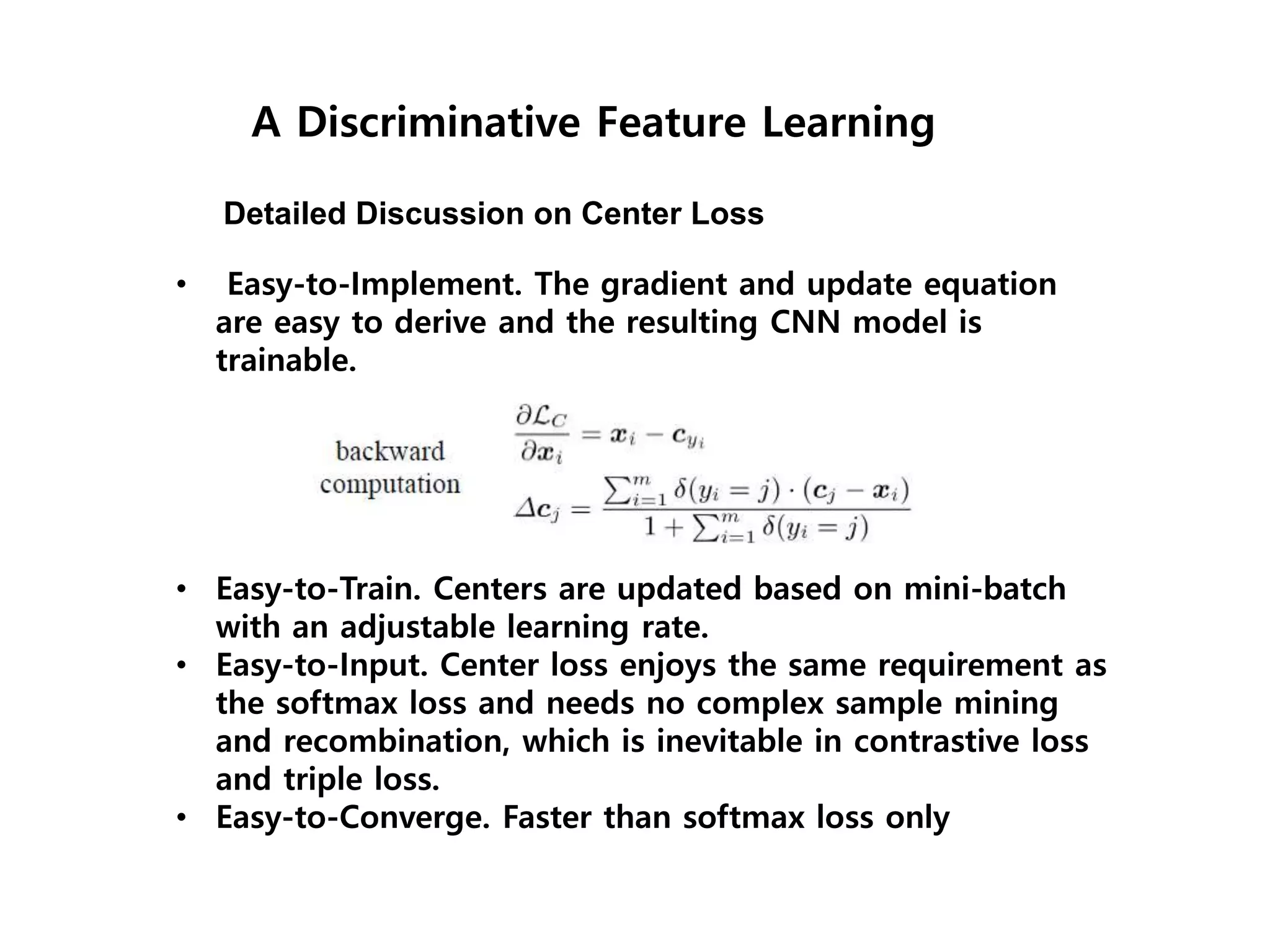
![Both MNIST and CIFAR-10 have ten different classes from which we create ten one-class classification setups. In each setup, one of the classes is the normal class and samples from the remaining classes are used to represent anomalies. Only train with training set examples from the respective normal class. Training set sizes of n≈6,000 for MNIST and n=5,000 for CIFAR-10. Both test sets have 10,000 samples including samples from the nine anomalous classes for each setup. Pre-process all images with global contrast normalization using the L1 norm and finally rescale to [0; 1] via min-max-scaling. One-class classification on MNIST and CIFAR-10 Data setup](https://image.slidesharecdn.com/anomalydetectionusingdeeponeclassclassifier-190309014237/75/Anomaly-detection-using-deep-one-class-classifier-87-2048.jpg)