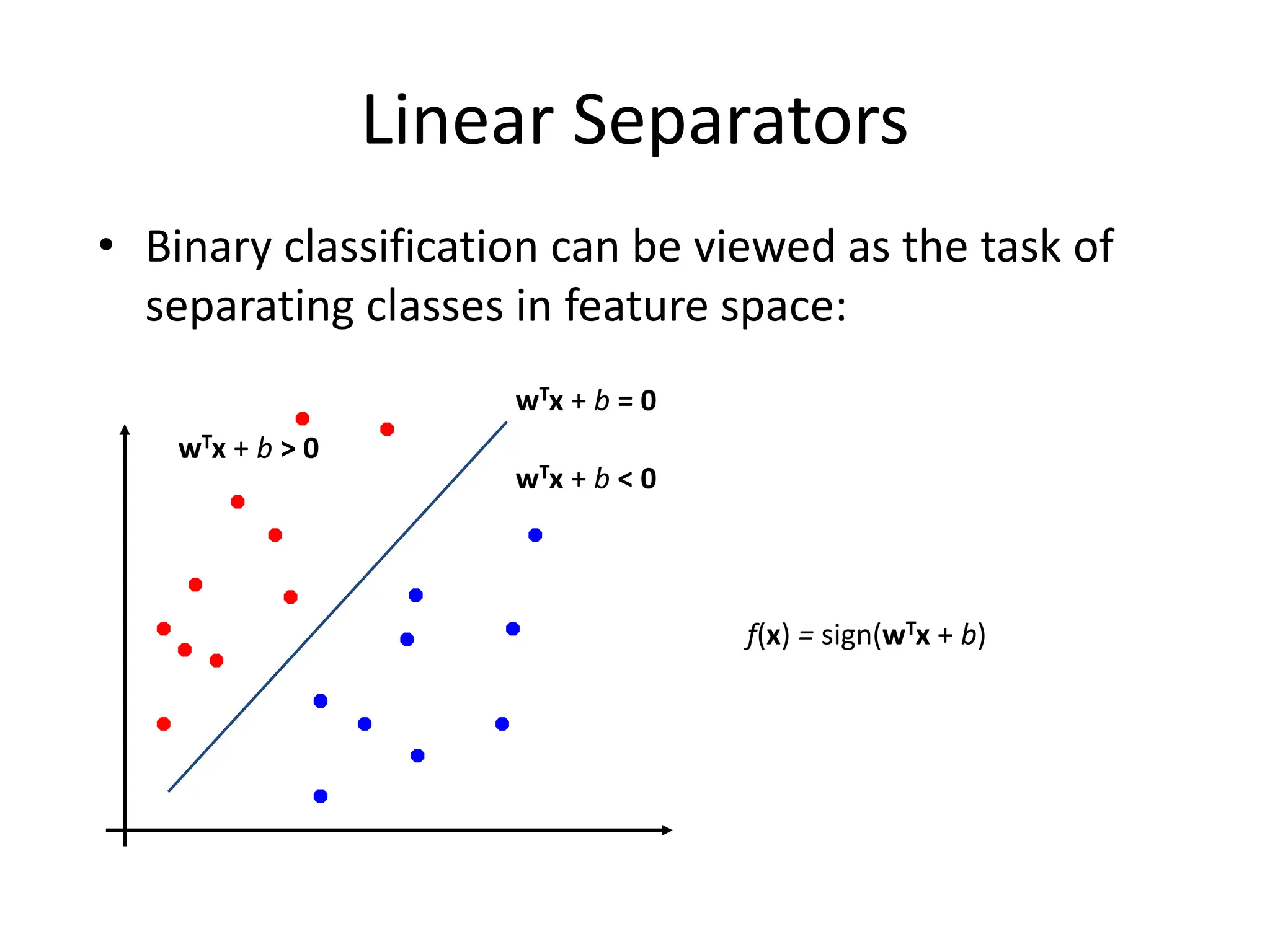
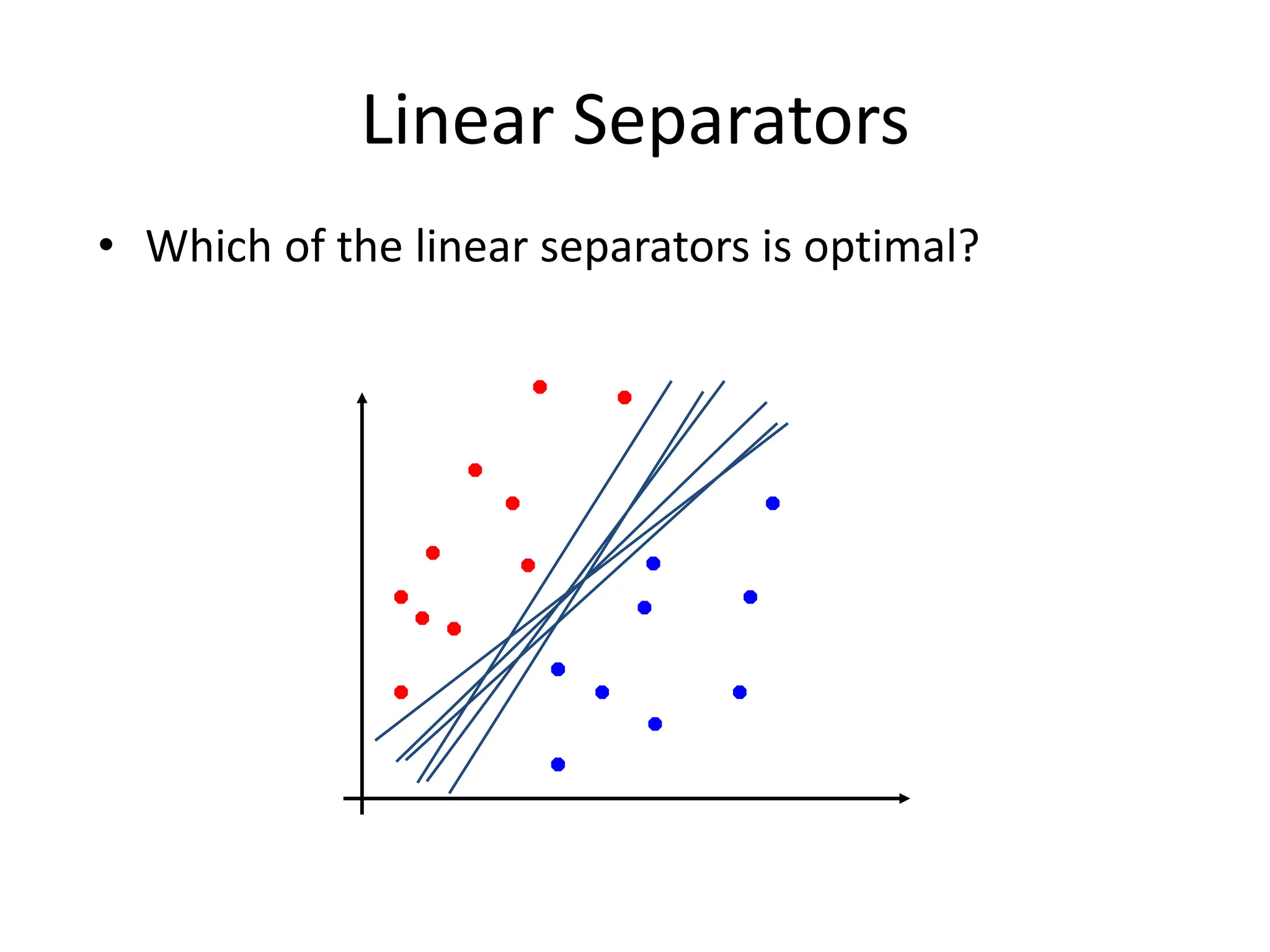
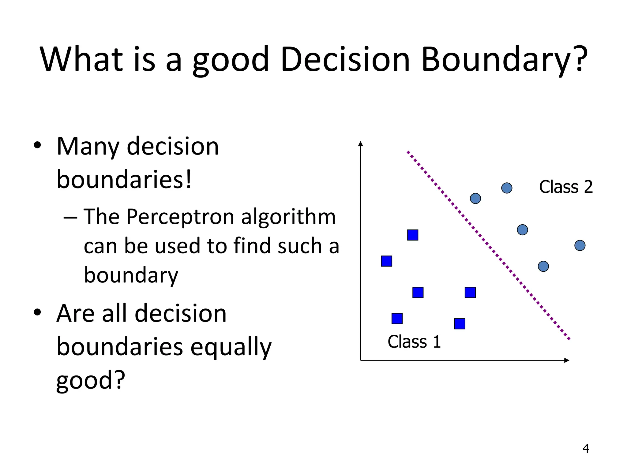
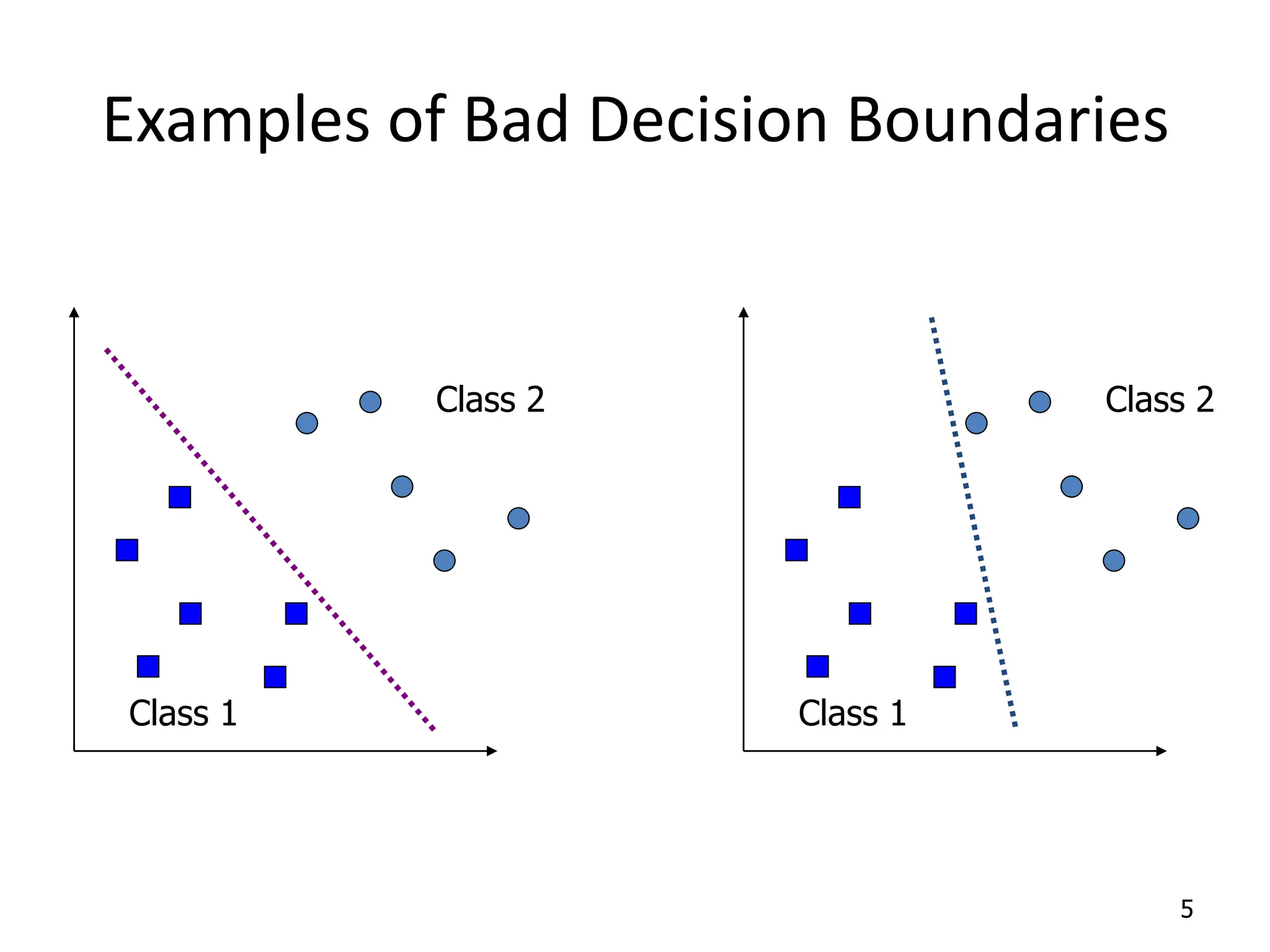
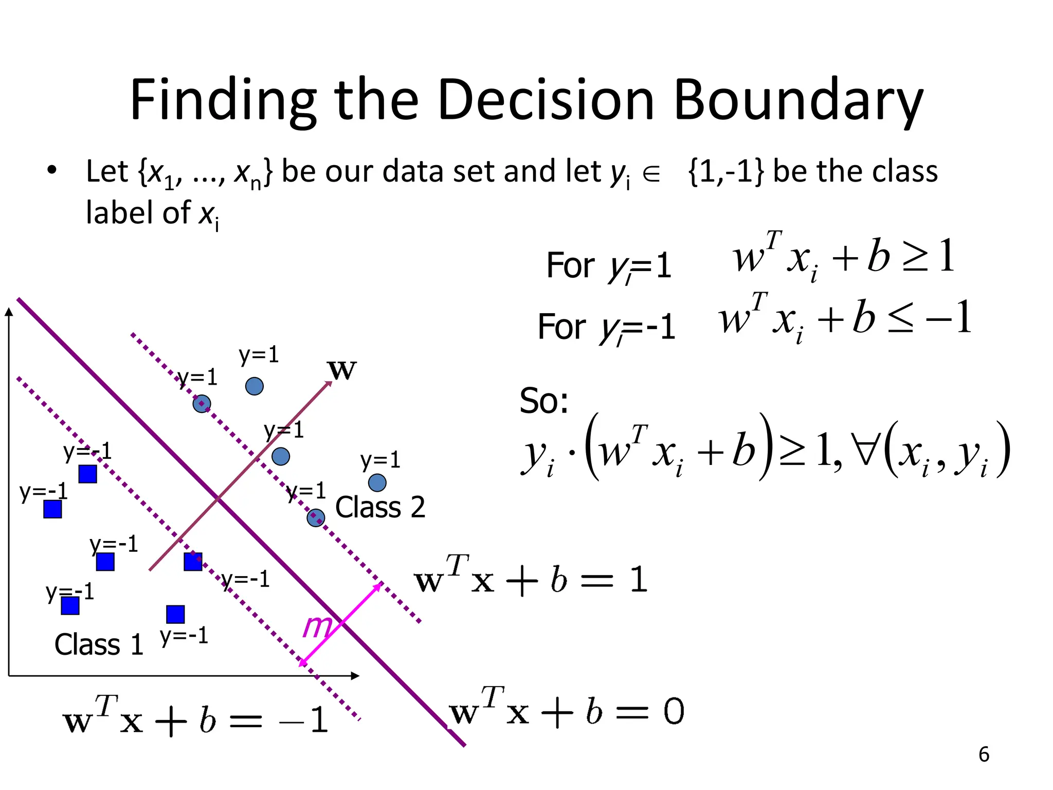
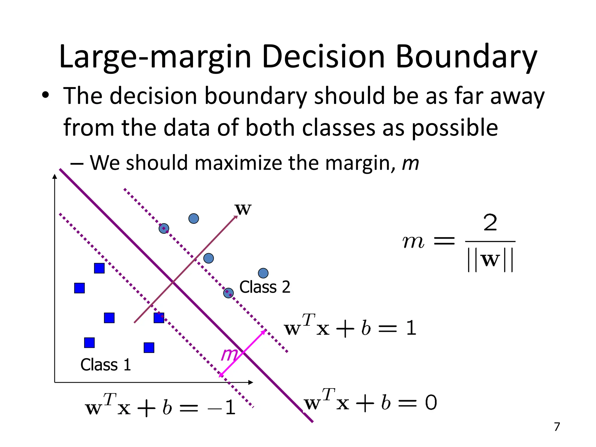
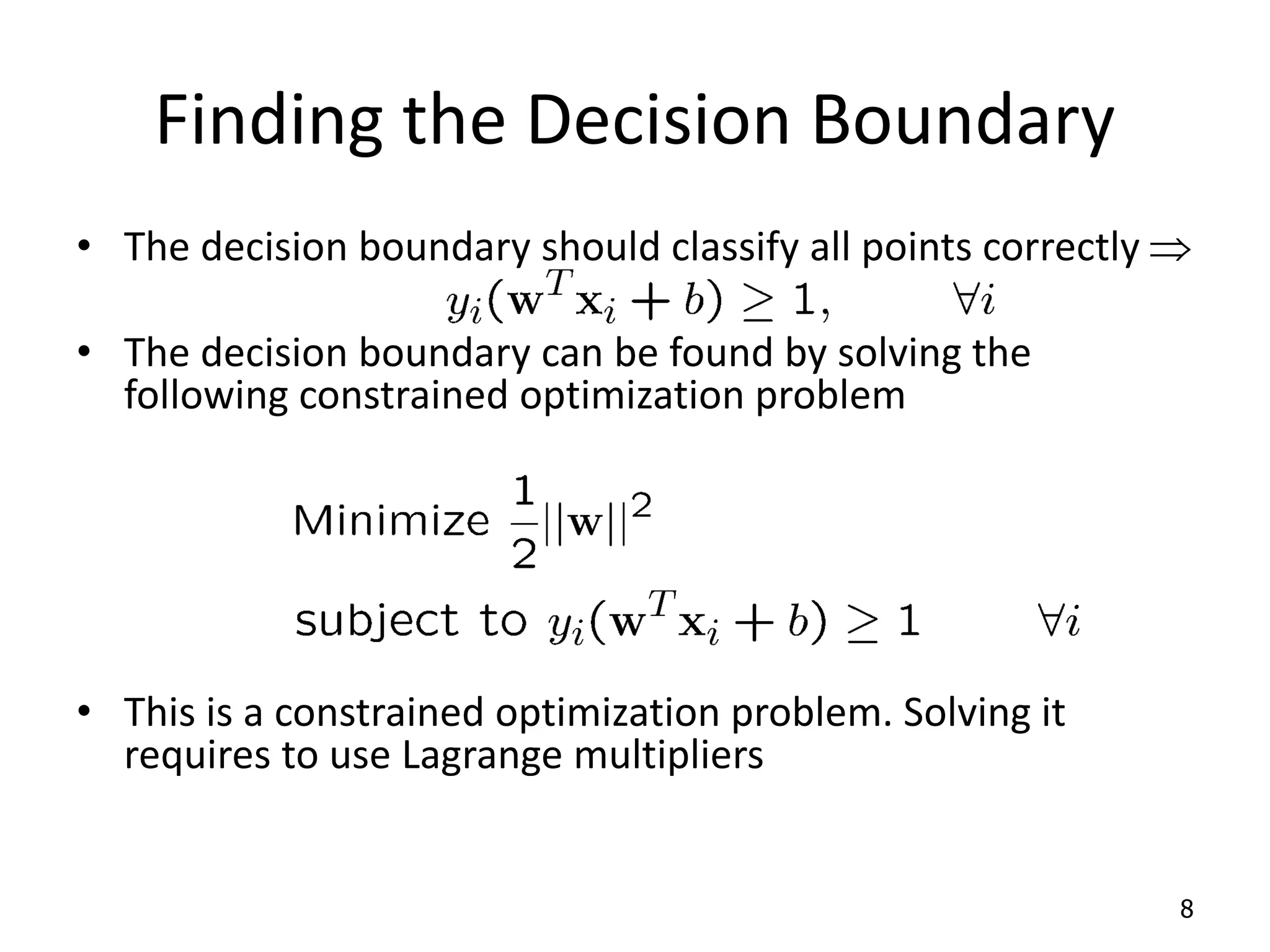
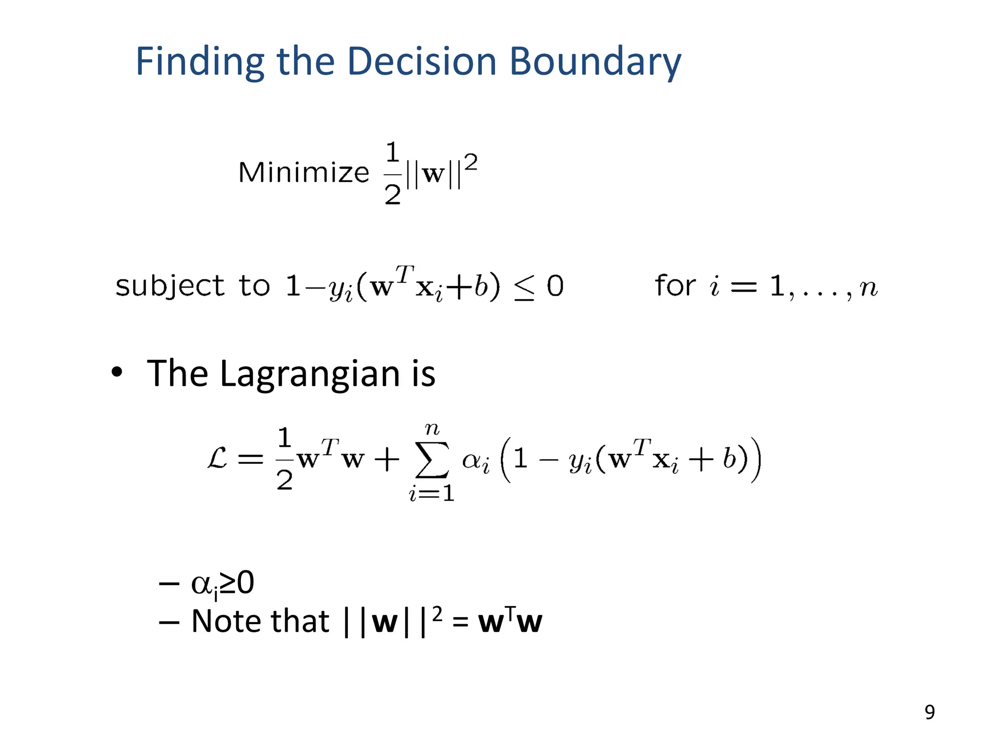
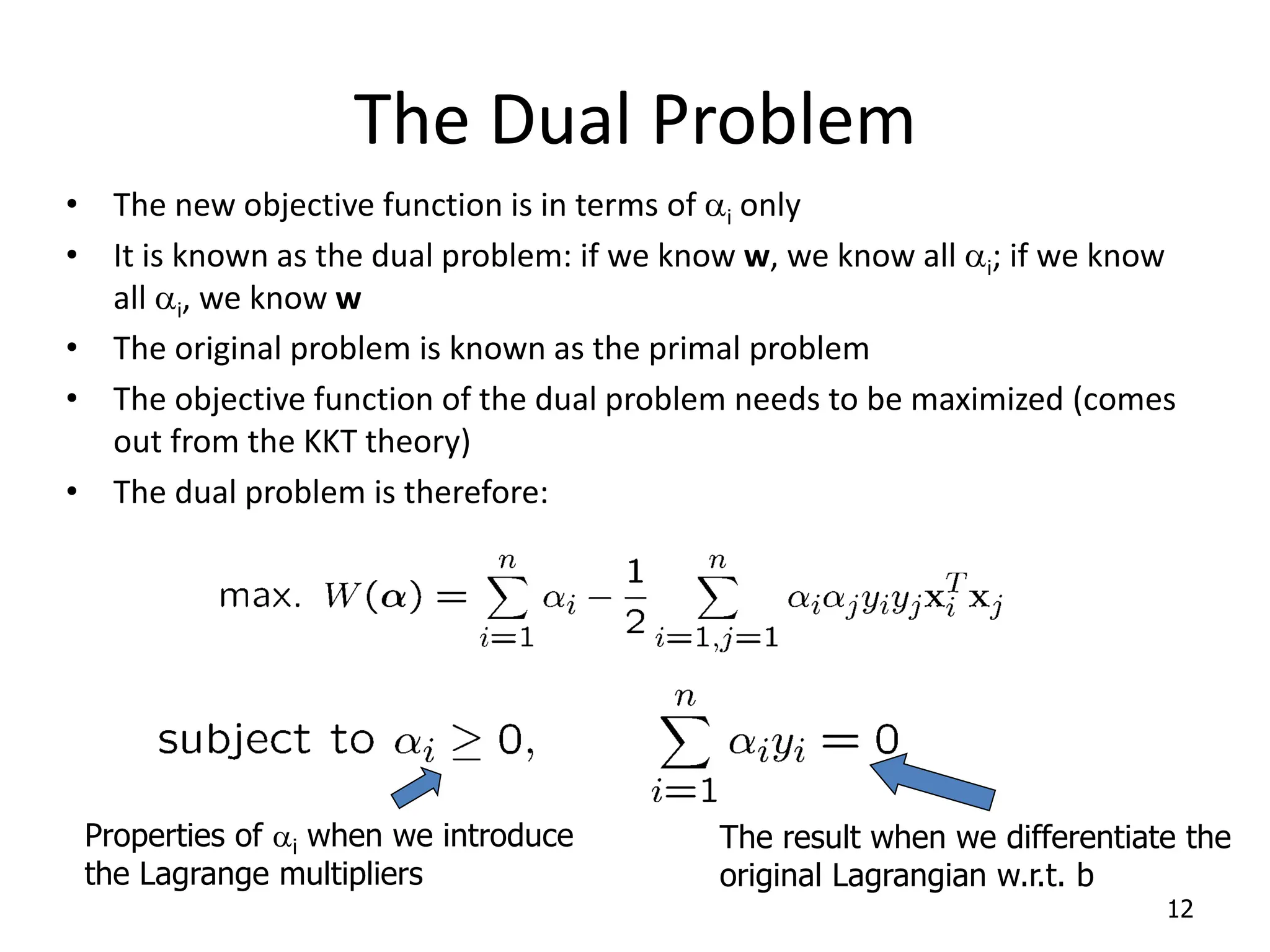
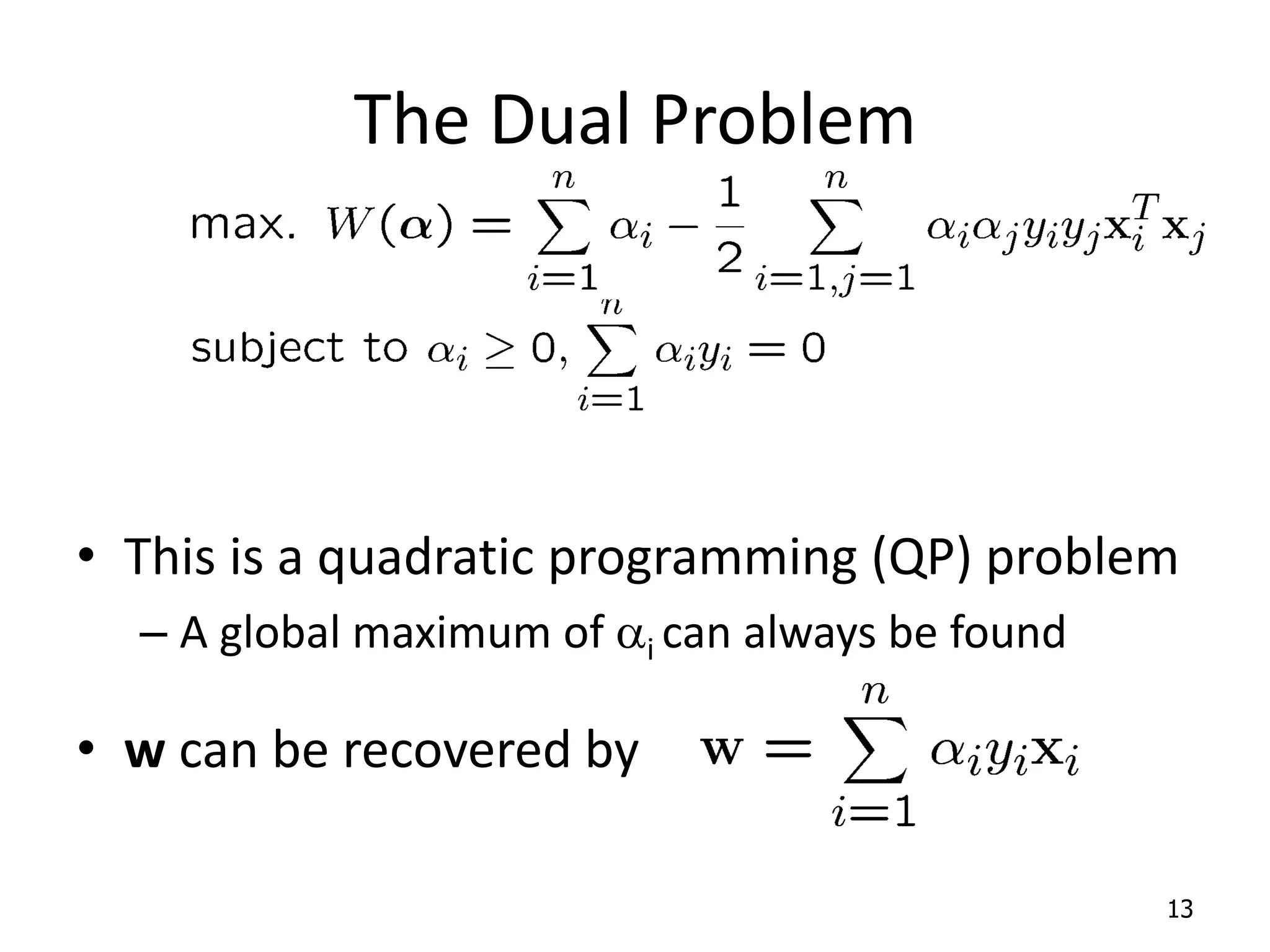
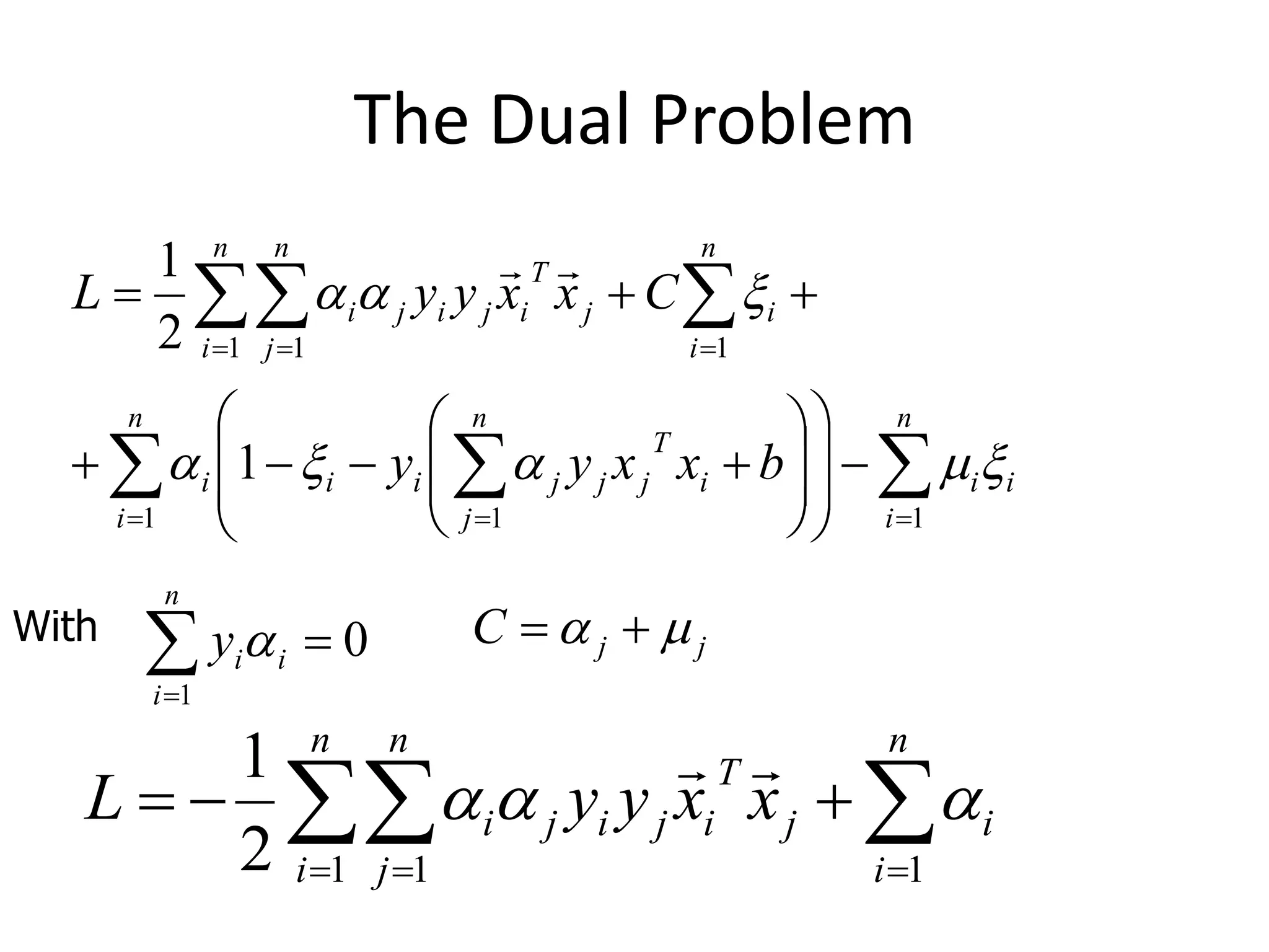
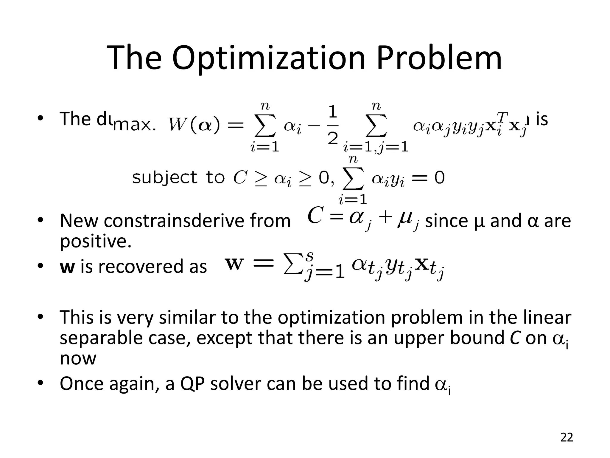
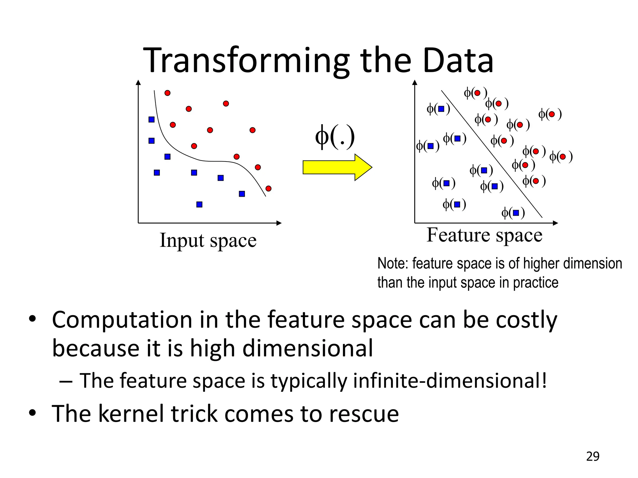
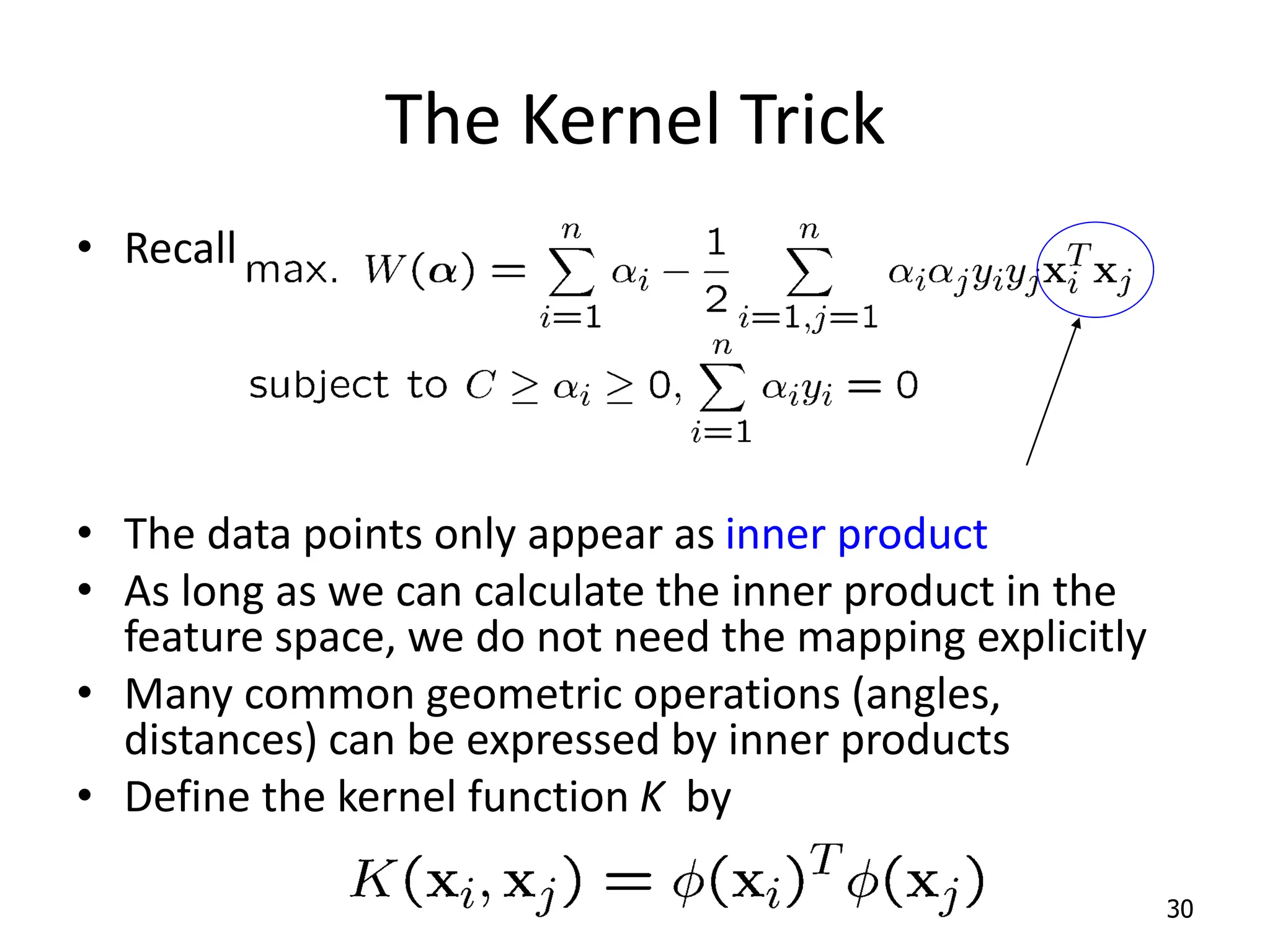
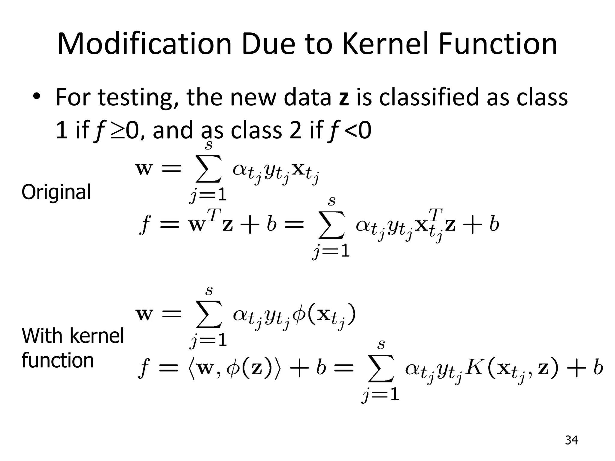
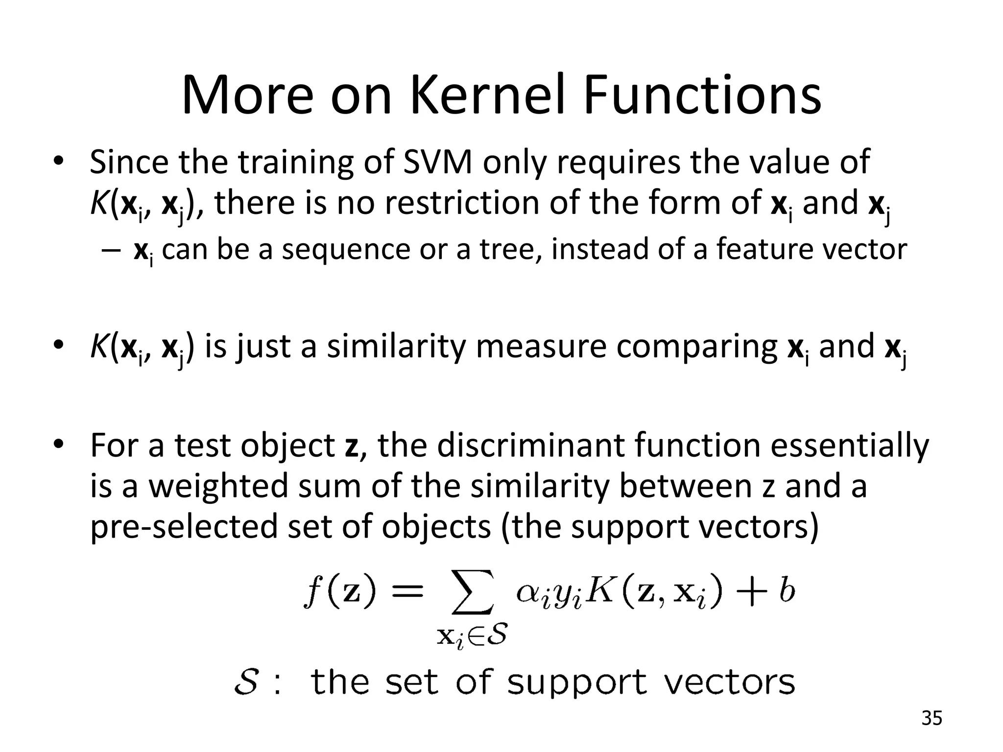
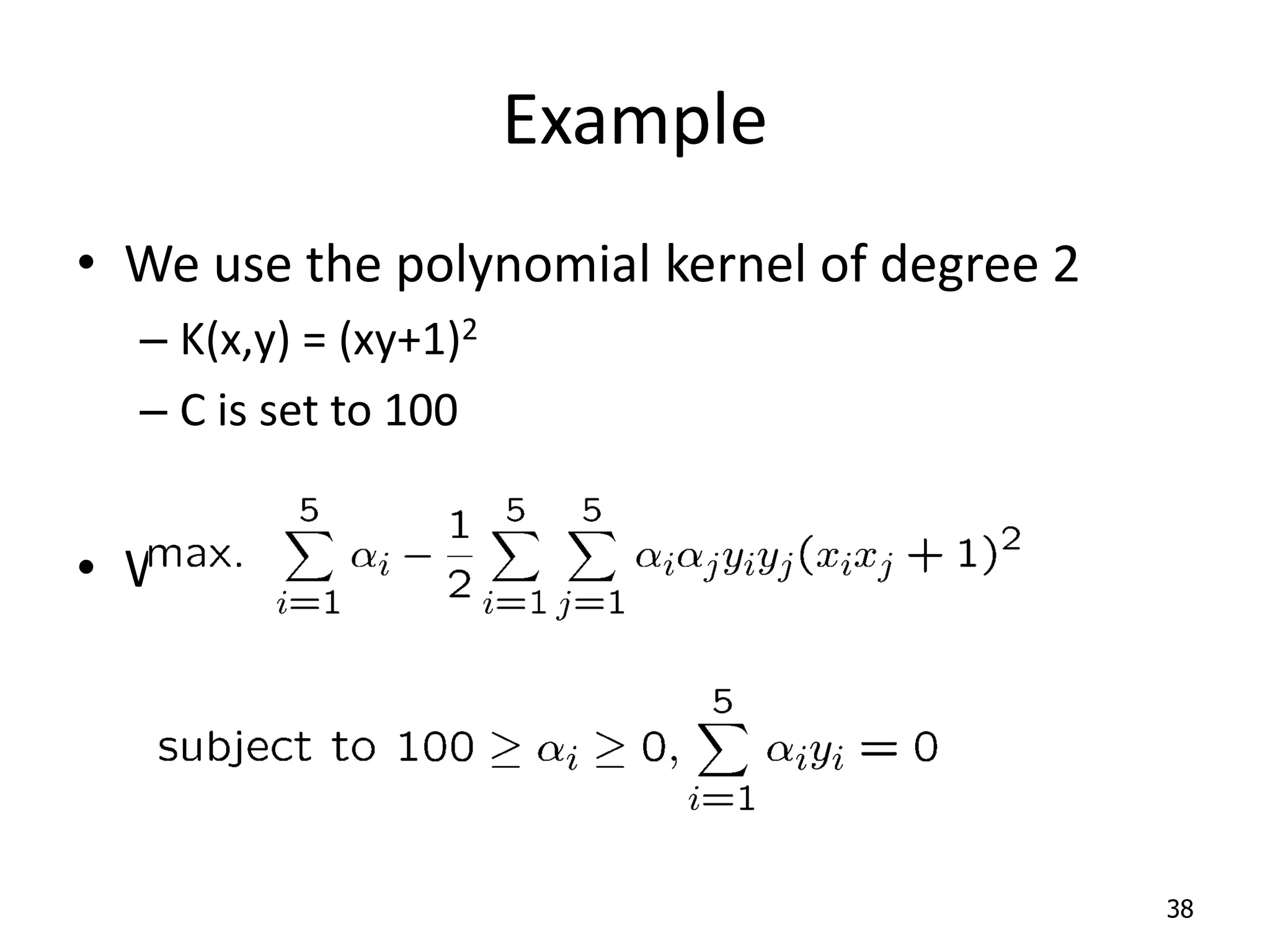
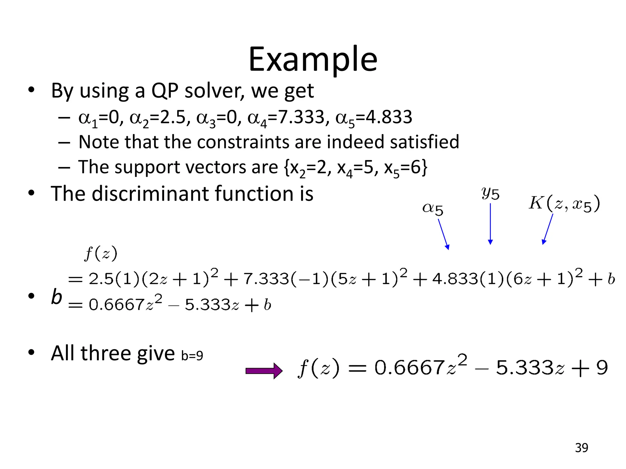
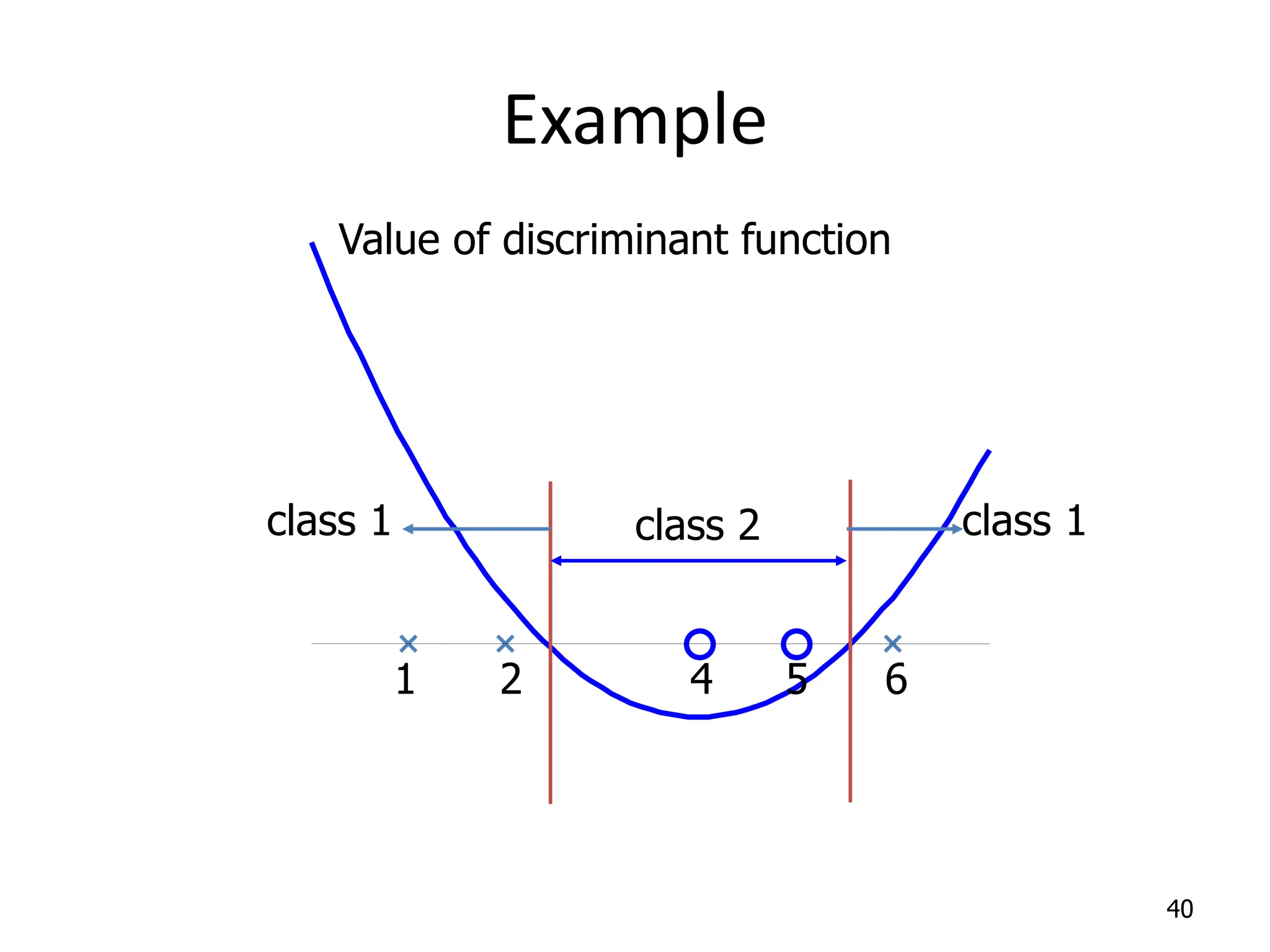
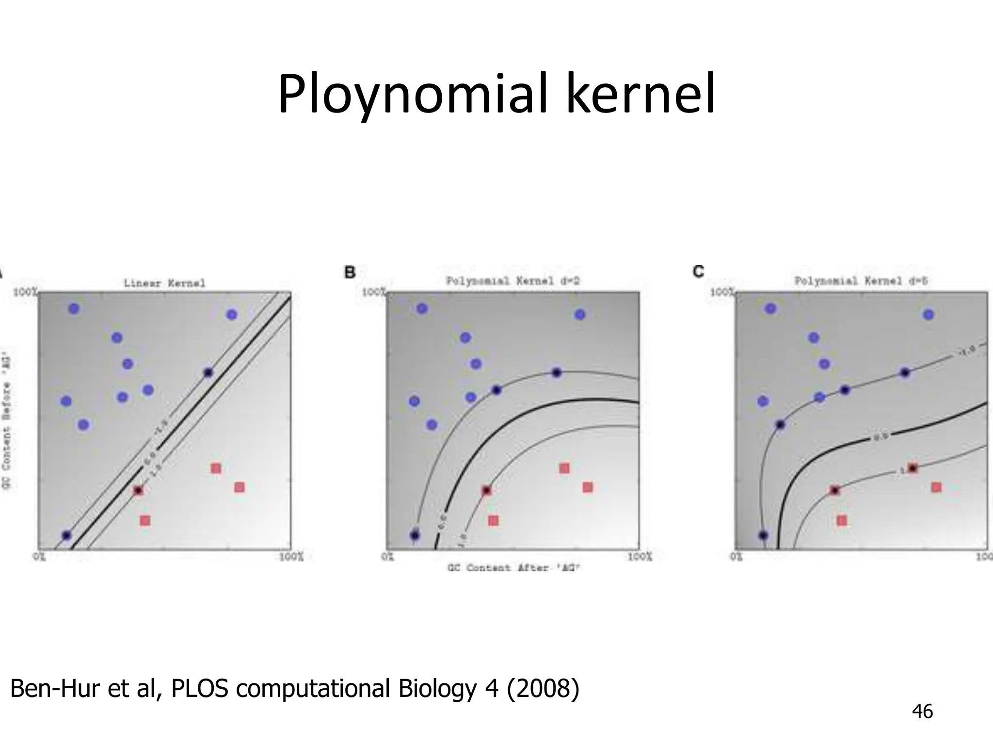
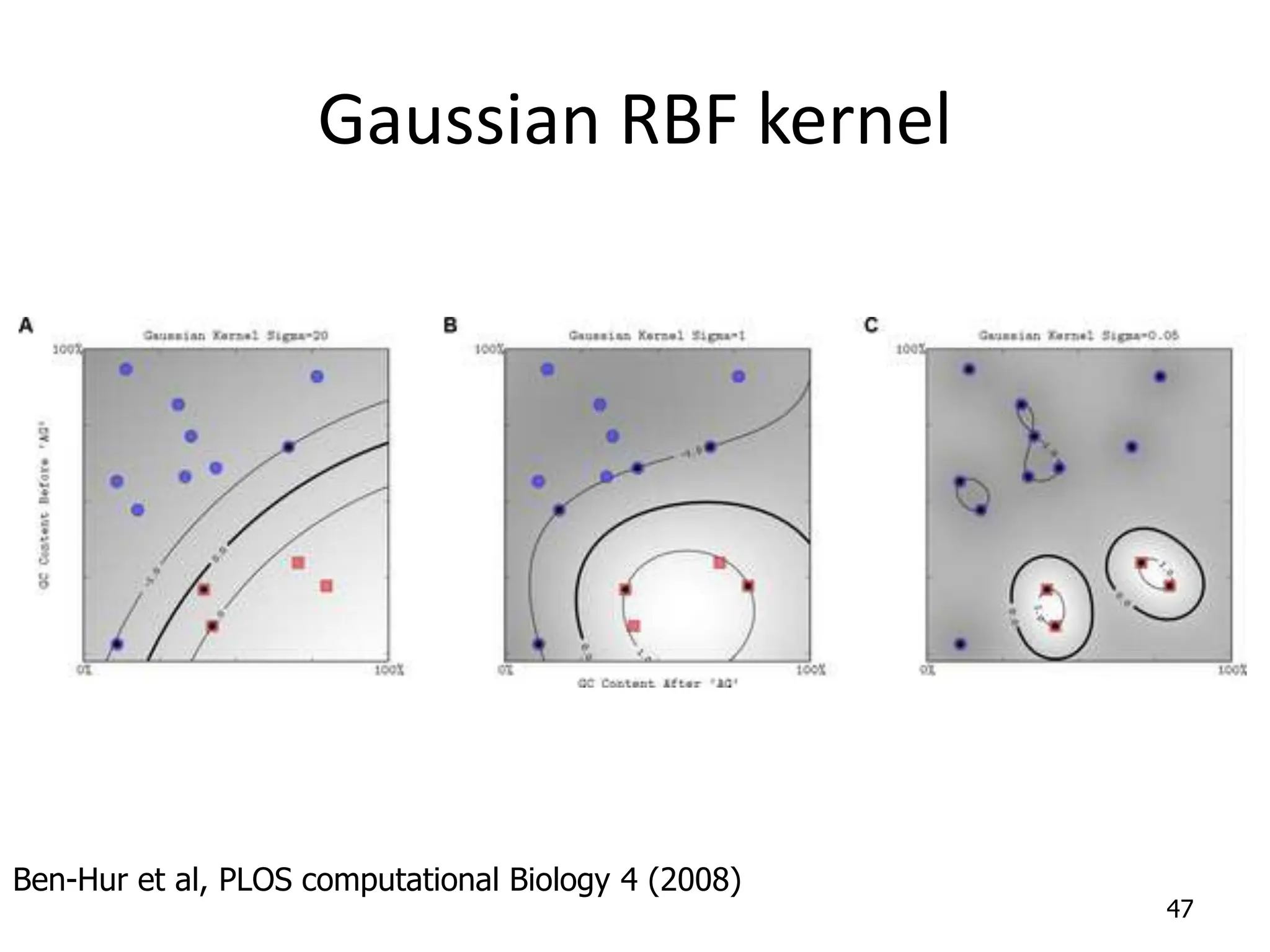
super vector machines algorithms using deep

Linear Separators • Binary classification can be viewed as the task of separating classes in feature space: wTx + b = 0 wTx + b < 0 wTx + b > 0 f(x) = sign(wTx + b)

Linear Separators • Which of the linear separators is optimal?

What is a good Decision Boundary? • Many decision boundaries! – The Perceptron algorithm can be used to find such a boundary • Are all decision boundaries equally good? 4 Class 1 Class 2

Examples of Bad Decision Boundaries 5 Class 1 Class 2 Class 1 Class 2

Finding the Decision Boundary • Let {x1, ..., xn} be our data set and let yi  {1,-1} be the class label of xi 6 Class 1 Class 2 m y=1 y=1 y=1 y=1 y=1 y=-1 y=-1 y=-1 y=-1 y=-1 y=-1 1   b x w i T For yi=1 1    b x w i T For yi=-1     i i i T i y x b x w y , , 1     So:

Large-margin Decision Boundary • The decision boundary should be as far away from the data of both classes as possible – We should maximize the margin, m 7 Class 1 Class 2 m

Finding the Decision Boundary • The decision boundary should classify all points correctly  • The decision boundary can be found by solving the following constrained optimization problem • This is a constrained optimization problem. Solving it requires to use Lagrange multipliers 8

• The Lagrangian is – ai≥0 – Note that ||w||2 = wTw 9 Finding the Decision Boundary

• Setting the gradient of w.r.t. w and b to zero, we have 10 Gradient with respect to w and b               0 , 0 b L k w L k                                    n i m k k i k i i m k k k n i i T i i T b x w y w w b x w y w w L 1 1 1 1 1 2 1 1 2 1 a a n: no of examples, m: dimension of the space

The Dual Problem • If we substitute to , we have Since • This is a function of ai only 11

The Dual Problem • The new objective function is in terms of ai only • It is known as the dual problem: if we know w, we know all ai; if we know all ai, we know w • The original problem is known as the primal problem • The objective function of the dual problem needs to be maximized (comes out from the KKT theory) • The dual problem is therefore: 12 Properties of ai when we introduce the Lagrange multipliers The result when we differentiate the original Lagrangian w.r.t. b

The Dual Problem • This is a quadratic programming (QP) problem – A global maximum of ai can always be found • w can be recovered by 13

Characteristics of the Solution • Many of the ai are zero – w is a linear combination of a small number of data points – This “sparse” representation can be viewed as data compression as in the construction of knn classifier • xi with non-zero ai are called support vectors (SV) – The decision boundary is determined only by the SV – Let tj (j=1, ..., s) be the indices of the s support vectors. We can write – Note: w need not be formed explicitly 14

A Geometrical Interpretation 15 a6=1.4 Class 1 Class 2 a1=0.8 a2=0 a3=0 a4=0 a5=0 a7=0 a8=0.6 a9=0 a10=0

Characteristics of the Solution • For testing with a new data z – Compute and classify z as class 1 if the sum is positive, and class 2 otherwise – Note: w need not be formed explicitly 16

The Quadratic Programming Problem • Many approaches have been proposed – Loqo, cplex, etc. (see http://www.numerical.rl.ac.uk/qp/qp.html) • Most are “interior-point” methods – Start with an initial solution that can violate the constraints – Improve this solution by optimizing the objective function and/or reducing the amount of constraint violation • For SVM, sequential minimal optimization (SMO) seems to be the most popular – A QP with two variables is trivial to solve – Each iteration of SMO picks a pair of (ai,aj) and solve the QP with these two variables; repeat until convergence • In practice, we can just regard the QP solver as a “black- box” without bothering how it works 17

Non-linearly Separable Problems • We allow “error” xi in classification; it is based on the output of the discriminant function wTx+b • xi approximates the number of misclassified samples 18 Class 1 Class 2

Soft Margin Hyperplane • The new conditions become – xi are “slack variables” in optimization – Note that xi=0 if there is no error for xi – xi is an upper bound of the number of errors • We want to minimize • C : tradeoff parameter between error and margin 19    n i i C w 1 2 2 1 x

The Optimization Problem 20                  n i i i n i i T i i i n i i T b x w y C w w L 1 1 1 1 2 1 x  x a x 0 1        n i ij i i j j x y w w L a 0 1     n i i i i x y w   a 0       j j j C L  a x 0 1       n i i i y b L a With α and μ Lagrange multipliers, POSITIVE

The Dual Problem         n i i j T i j i n i n j j i x x y y L 1 1 1 2 1 a a a                                      n i i i n i n j i T j j j i i i n i i j T i j i n i n j j i b x x y y C x x y y L 1 1 1 1 1 1 1 2 1 x  a x a x a a   j j C  a   0 1    n i i i y a With

The Optimization Problem • The dual of this new constrained optimization problem is • New constrainsderive from since μ and α are positive. • w is recovered as • This is very similar to the optimization problem in the linear separable case, except that there is an upper bound C on ai now • Once again, a QP solver can be used to find ai 22 j j C  a  

• The algorithm try to keep ξ null, maximising the margin • The algorithm does not minimise the number of error. Instead, it minimises the sum of distances fron the hyperplane • When C increases the number of errors tend to lower. At the limit of C tending to infinite, the solution tend to that given by the hard margin formulation, with 0 errors 3/11/2024 23    n i i C w 1 2 2 1 x

Extension to Non-linear Decision Boundary • So far, we have only considered large-margin classifier with a linear decision boundary • How to generalize it to become nonlinear? • Key idea: transform xi to a higher dimensional space to “make life easier” – Input space: the space the point xi are located – Feature space: the space of f(xi) after transformation • Why transform? – Linear operation in the feature space is equivalent to non-linear operation in input space – Classification can become easier with a proper transformation. In the XOR problem, for example, adding a new feature of x1x2 make the problem linearly separable 25

XOR X Y 0 0 0 0 1 1 1 0 1 1 1 0 26 Is not linearly separable X Y XY 0 0 0 0 0 1 0 1 1 0 0 1 1 1 1 0 Is linearly separable

Transforming the Data • Computation in the feature space can be costly because it is high dimensional – The feature space is typically infinite-dimensional! • The kernel trick comes to rescue 28 f( ) f( ) f( ) f( ) f( ) f( ) f( ) f( ) f(.) f( ) f( ) f( ) f( ) f( ) f( ) f( ) f( ) f( ) f( ) Feature space Input space Note: feature space is of higher dimension than the input space in practice

Transforming the Data • Computation in the feature space can be costly because it is high dimensional – The feature space is typically infinite-dimensional! • The kernel trick comes to rescue 29 f( ) f( ) f( ) f( ) f( ) f( ) f( ) f( ) f(.) f( ) f( ) f( ) f( ) f( ) f( ) f( ) f( ) f( ) f( ) Feature space Input space Note: feature space is of higher dimension than the input space in practice

The Kernel Trick • Recall the SVM optimization problem • The data points only appear as inner product • As long as we can calculate the inner product in the feature space, we do not need the mapping explicitly • Many common geometric operations (angles, distances) can be expressed by inner products • Define the kernel function K by 30

An Example for f(.) and K(.,.) • Suppose f(.) is given as follows • An inner product in the feature space is • So, if we define the kernel function as follows, there is no need to carry out f(.) explicitly • This use of kernel function to avoid carrying out f(.) explicitly is known as the kernel trick 31

Kernels • Given a mapping: a kernel is represented as the inner product A kernel must satisfy the Mercer’s condition: 32 φ(x) x    i i i φ φ K (y) (x) y x ) , (       0 ) ( ) ( ) ( 0 ) ( such that ) ( 2 y x y x y x, x x x d d g g K d g g

Modification Due to Kernel Function • Change all inner products to kernel functions • For training, 33 Original With kernel function

Modification Due to Kernel Function • For testing, the new data z is classified as class 1 if f 0, and as class 2 if f <0 34 Original With kernel function

More on Kernel Functions • Since the training of SVM only requires the value of K(xi, xj), there is no restriction of the form of xi and xj – xi can be a sequence or a tree, instead of a feature vector • K(xi, xj) is just a similarity measure comparing xi and xj • For a test object z, the discriminant function essentially is a weighted sum of the similarity between z and a pre-selected set of objects (the support vectors) 35

Example • Suppose we have 5 1D data points – x1=1, x2=2, x3=4, x4=5, x5=6, with 1, 2, 6 as class 1 and 4, 5 as class 2  y1=1, y2=1, y3=-1, y4=-1, y5=1 36

Example 37 1 2 4 5 6 class 2 class 1 class 1

Example • We use the polynomial kernel of degree 2 – K(x,y) = (xy+1)2 – C is set to 100 • We first find ai (i=1, …, 5) by 38

Example • By using a QP solver, we get – a1=0, a2=2.5, a3=0, a4=7.333, a5=4.833 – Note that the constraints are indeed satisfied – The support vectors are {x2=2, x4=5, x5=6} • The discriminant function is • b is recovered by solving f(2)=1 or by f(5)=-1 or by f(6)=1, • All three give b=9 39

Example 40 Value of discriminant function 1 2 4 5 6 class 2 class 1 class 1

Kernel Functions • In practical use of SVM, the user specifies the kernel function; the transformation f(.) is not explicitly stated • Given a kernel function K(xi, xj), the transformation f(.) is given by its eigenfunctions (a concept in functional analysis) – Eigenfunctions can be difficult to construct explicitly – This is why people only specify the kernel function without worrying about the exact transformation • Another view: kernel function, being an inner product, is really a similarity measure between the objects 41

A kernel is associated to a transformation – Given a kernel, in principle it should be recovered the transformation in the feature space that originates it. – K(x,y) = (xy+1)2= x2y2+2xy+1 It corresponds the transformation 3/11/2024 42            1 2 2 x x x

Examples of Kernel Functions • Polynomial kernel up to degree d • Polynomial kernel up to degree d • Radial basis function kernel with width s – The feature space is infinite-dimensional • Sigmoid with parameter k and q – It does not satisfy the Mercer condition on all k and q 43

Building new kernels • If k1(x,y) and k2(x,y) are two valid kernels then the following kernels are valid – Linear Combination – Exponential – Product – Polymomial tranfsormation (Q: polymonial with non negative coeffients) – Function product (f: any function) 45 ) , ( ) , ( ) , ( 2 2 1 1 y x k c y x k c y x k     ) , ( exp ) , ( 1 y x k y x k  ) , ( ) , ( ) , ( 2 1 y x k y x k y x k     ) , ( ) , ( 1 y x k Q y x k  ) ( ) , ( ) ( ) , ( 1 y f y x k x f y x k 

Ploynomial kernel Ben-Hur et al, PLOS computational Biology 4 (2008) 46

Gaussian RBF kernel Ben-Hur et al, PLOS computational Biology 4 (2008) 47

Spectral kernel for sequences • Given a DNA sequence x we can count the number of bases (4-D feature space) • Or the number of dimers (16-D space) • Or l-mers (4l –D space) • The spectral kernel is 3/11/2024 48 ) , , , ( ) ( 1 T G C A n n n n x  f ,..) , , , , , , , ( ) ( 2 CT CG CC CA AT AG AC AA n n n n n n n n x  f     y x y x k l l l f f   ) , (

Choosing the Kernel Function • Probably the most tricky part of using SVM. • The kernel function is important because it creates the kernel matrix, which summarizes all the data • Many principles have been proposed (diffusion kernel, Fisher kernel, string kernel, …) • There is even research to estimate the kernel matrix from available information • In practice, a low degree polynomial kernel or RBF kernel with a reasonable width is a good initial try • Note that SVM with RBF kernel is closely related to RBF neural networks, with the centers of the radial basis functions automatically chosen for SVM 49

Other Aspects of SVM • How to use SVM for multi-class classification? – One can change the QP formulation to become multi-class – More often, multiple binary classifiers are combined • See DHS 5.2.2 for some discussion – One can train multiple one-versus-all classifiers, or combine multiple pairwise classifiers “intelligently” • How to interpret the SVM discriminant function value as probability? – By performing logistic regression on the SVM output of a set of data (validation set) that is not used for training • Some SVM software (like libsvm) have these features built-in 50

Active Support Vector Learning P. Mitra, B. Uma Shankar and S. K. Pal, Segmentation of multispectral remote sensing Images using active support vector machines, Pattern Recognition Letters, 2004.

Software • A list of SVM implementation can be found at http://www.kernel- machines.org/software.html • Some implementation (such as LIBSVM) can handle multi-class classification • SVMLight is among one of the earliest implementation of SVM • Several Matlab toolboxes for SVM are also available 53

Summary: Steps for Classification • Prepare the pattern matrix • Select the kernel function to use • Select the parameter of the kernel function and the value of C – You can use the values suggested by the SVM software, or you can set apart a validation set to determine the values of the parameter • Execute the training algorithm and obtain the ai • Unseen data can be classified using the ai and the support vectors 54

Strengths and Weaknesses of SVM • Strengths – Training is relatively easy • No local optimal, unlike in neural networks – It scales relatively well to high dimensional data – Tradeoff between classifier complexity and error can be controlled explicitly – Non-traditional data like strings and trees can be used as input to SVM, instead of feature vectors • Weaknesses – Need to choose a “good” kernel function. 55

Conclusion • SVM is a useful alternative to neural networks • Two key concepts of SVM: maximize the margin and the kernel trick • Many SVM implementations are available on the web for you to try on your data set! 56

Resources • http://www.kernel-machines.org/ • http://www.support-vector.net/ • http://www.support-vector.net/icml- tutorial.pdf • http://www.kernel- machines.org/papers/tutorial-nips.ps.gz • http://www.clopinet.com/isabelle/Projects/SV M/applist.html 57

super vector machines algorithms using deep

More Related Content

Similar to super vector machines algorithms using deep

More from KNaveenKumarECE

Recently uploaded

super vector machines algorithms using deep