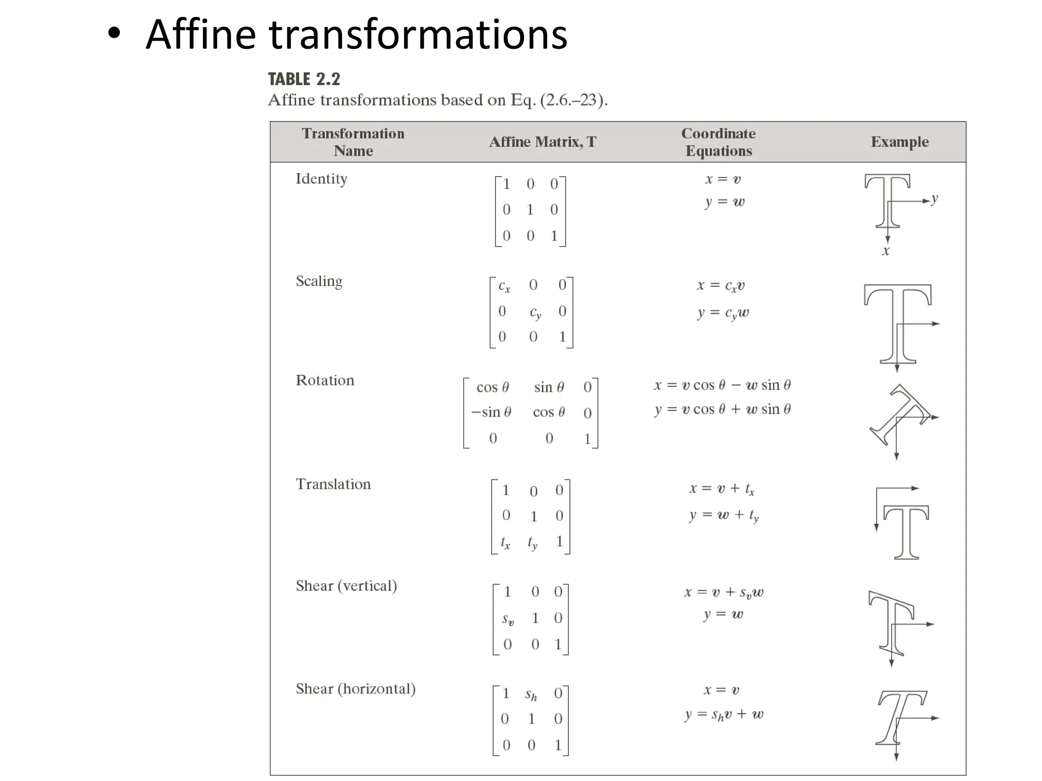
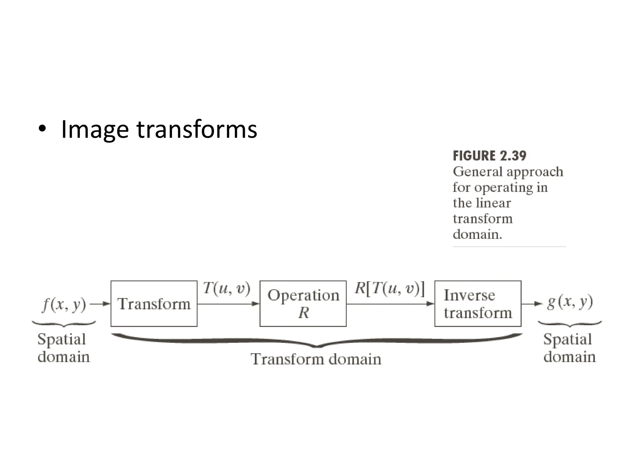
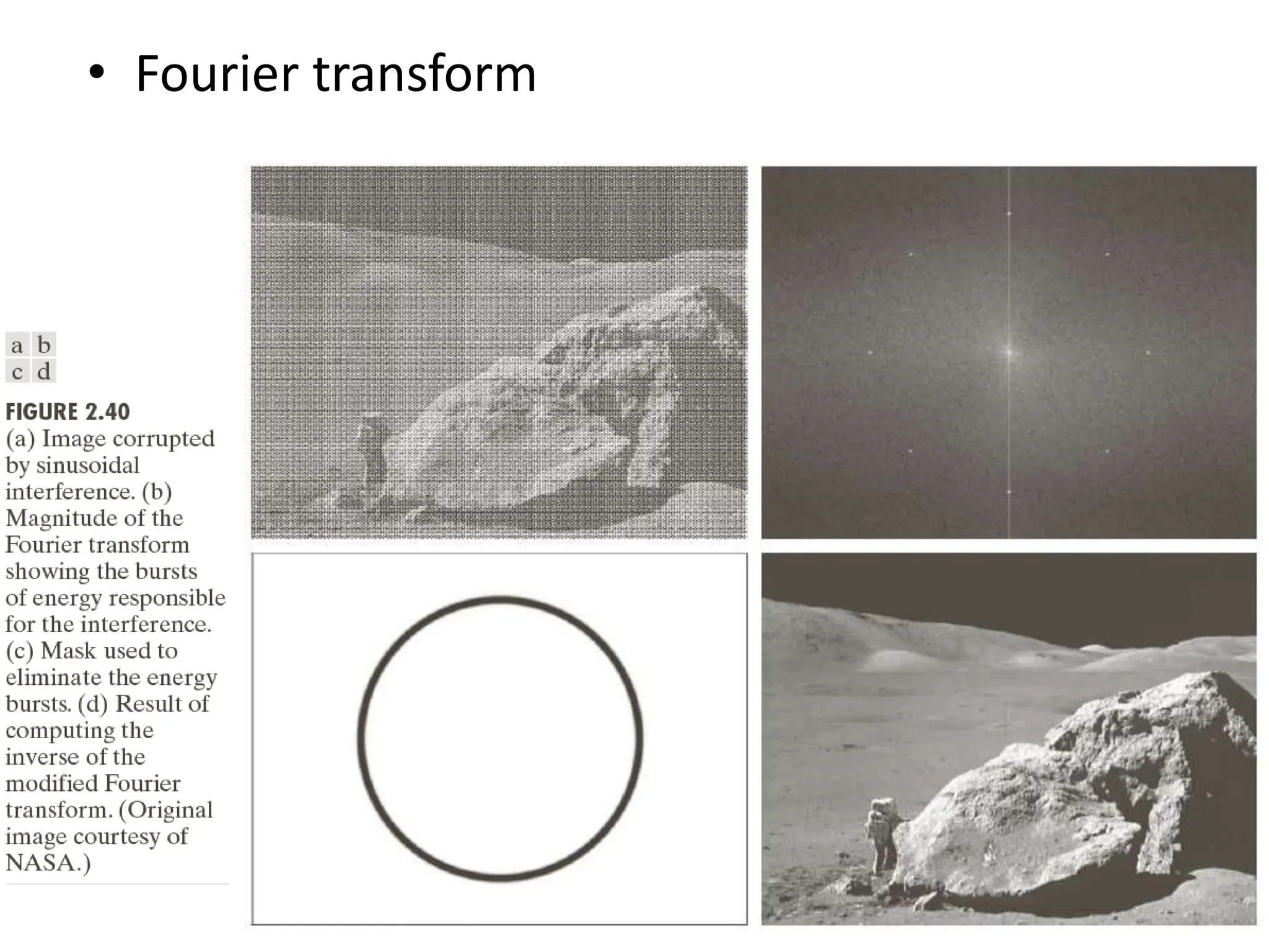
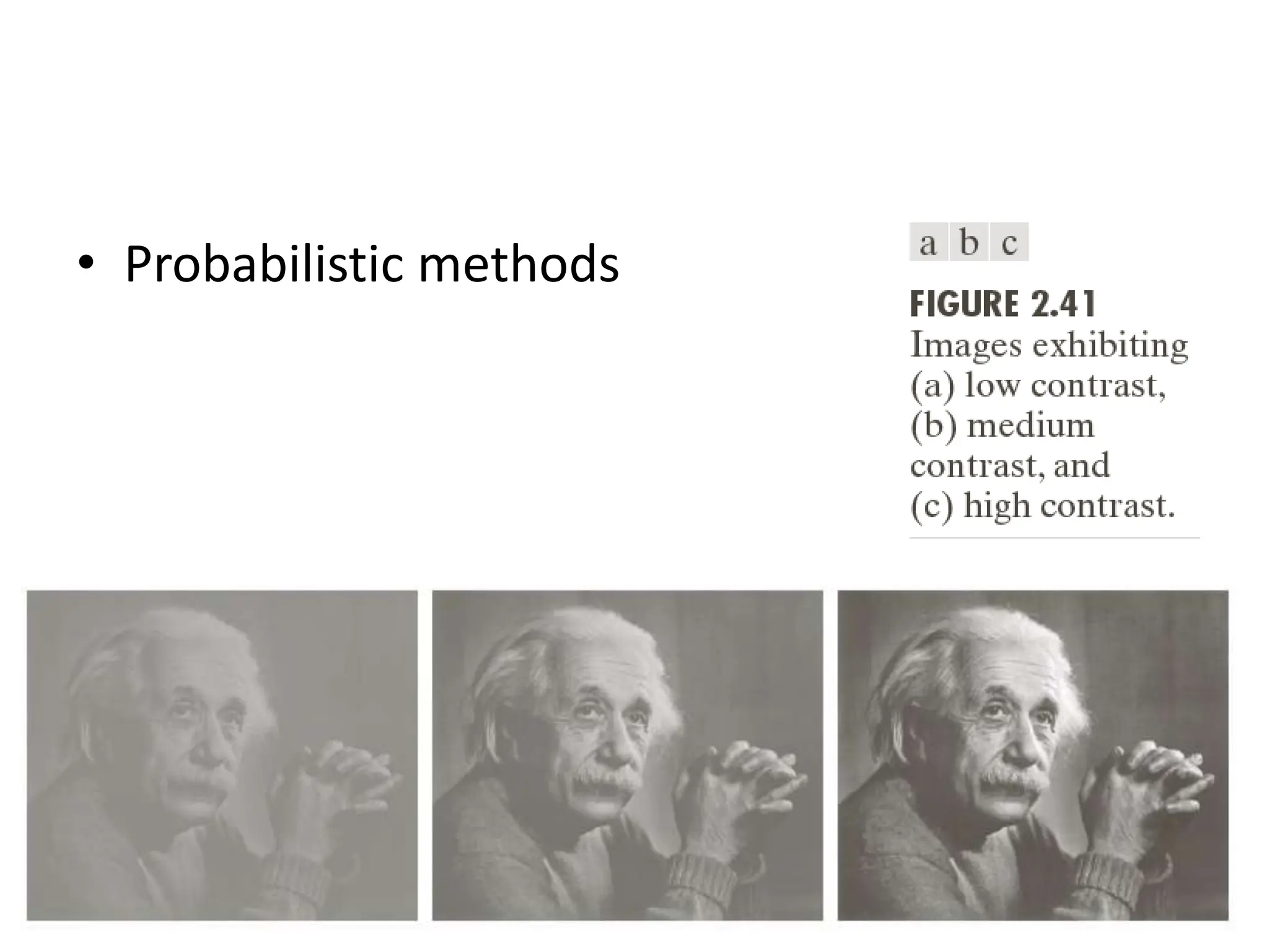
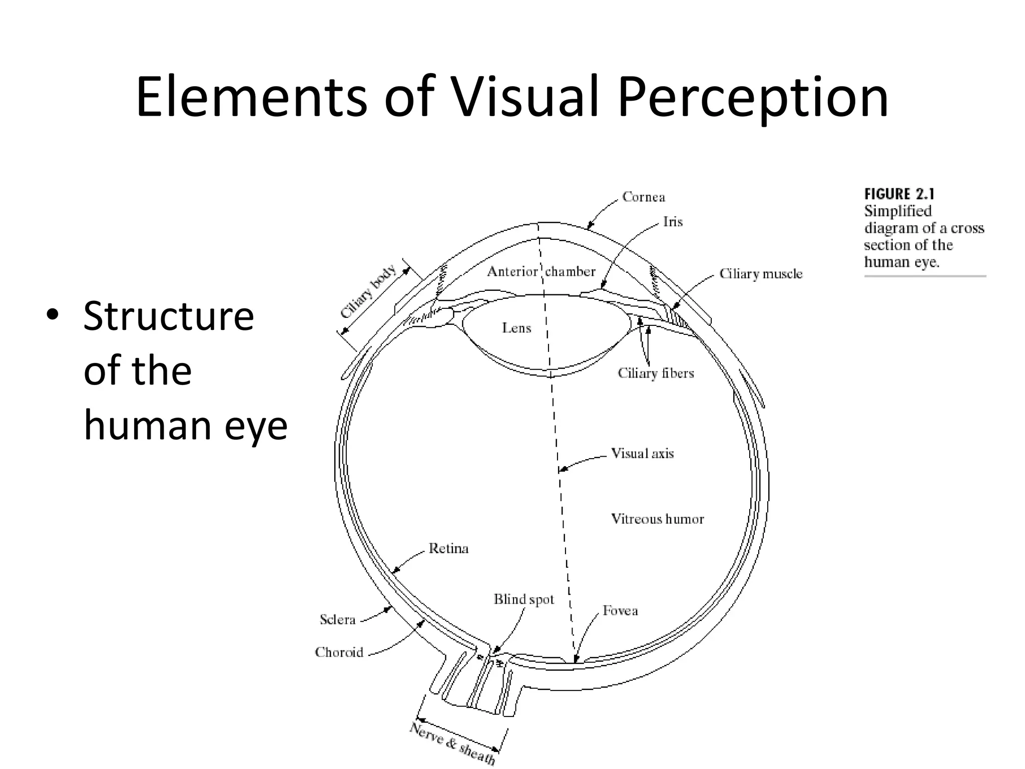
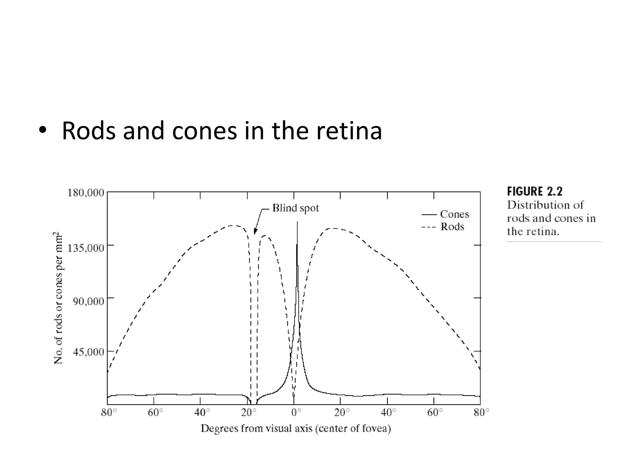
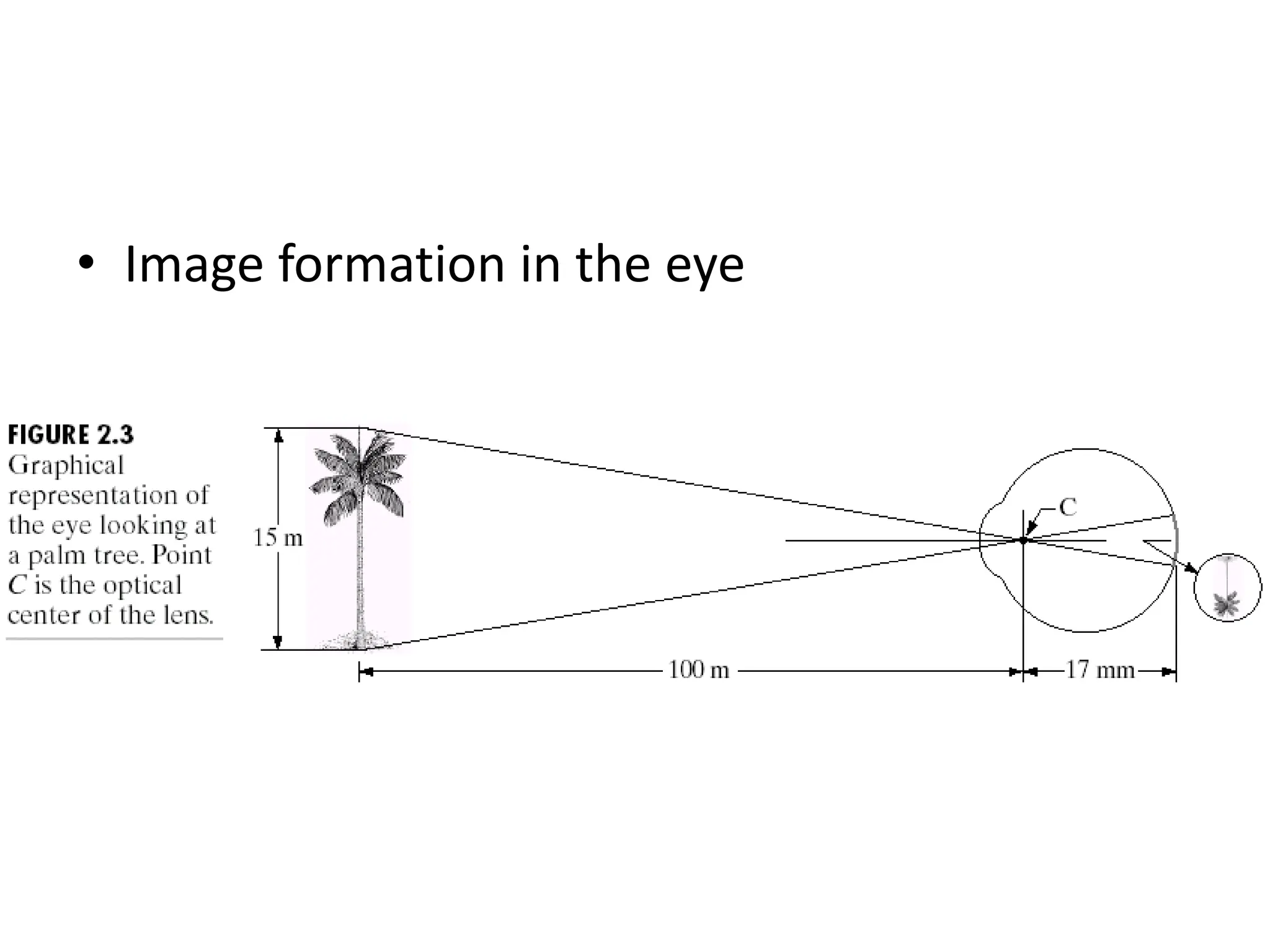
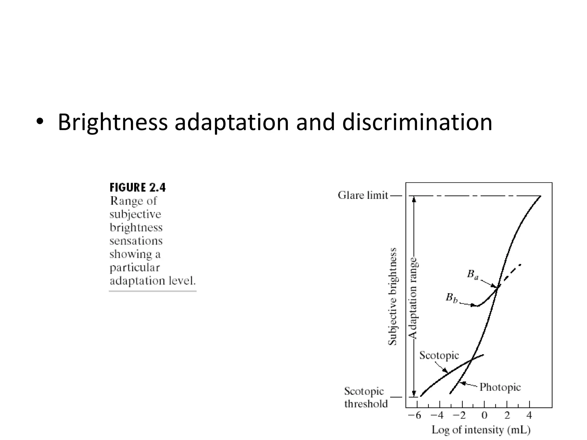
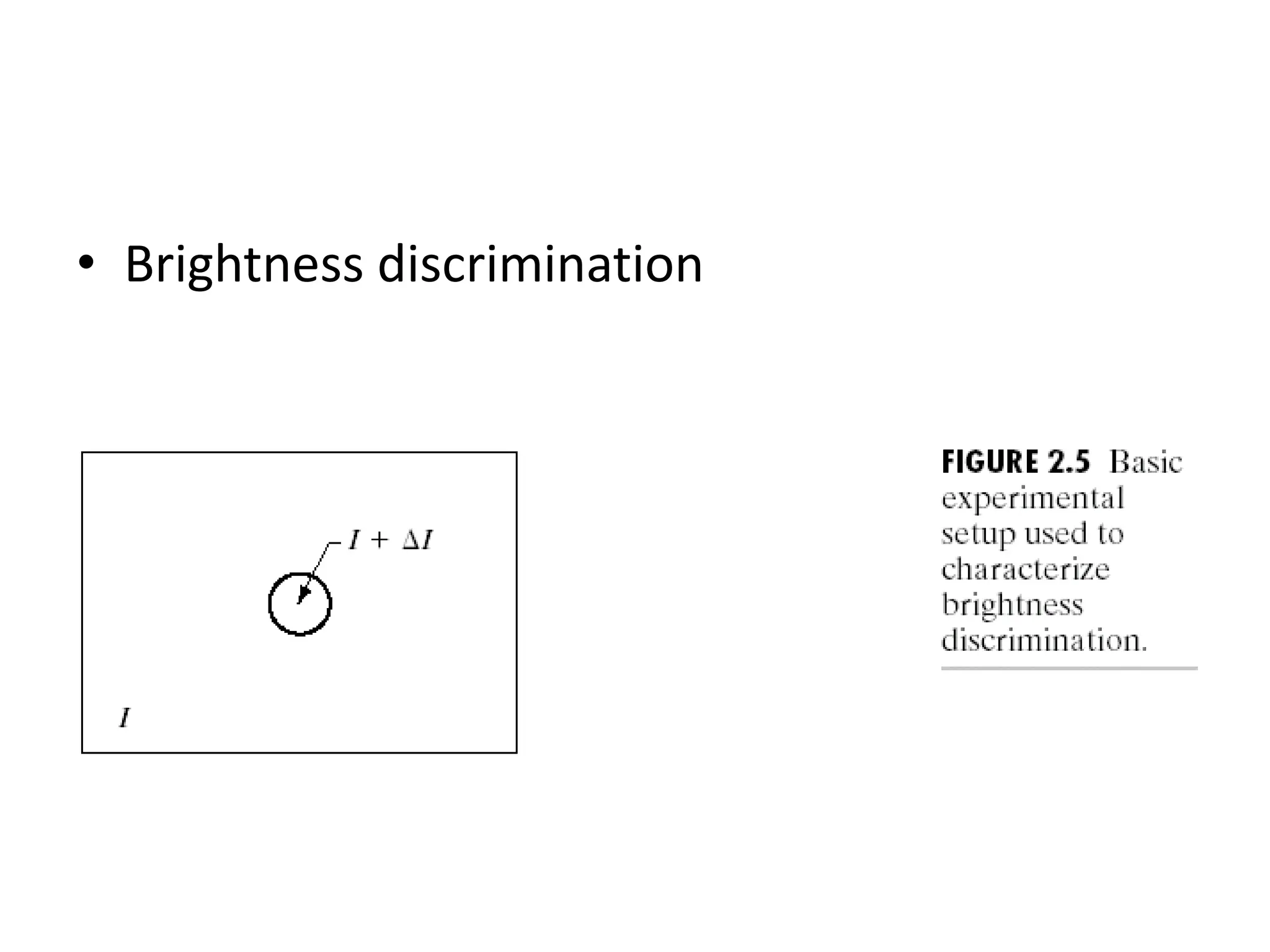
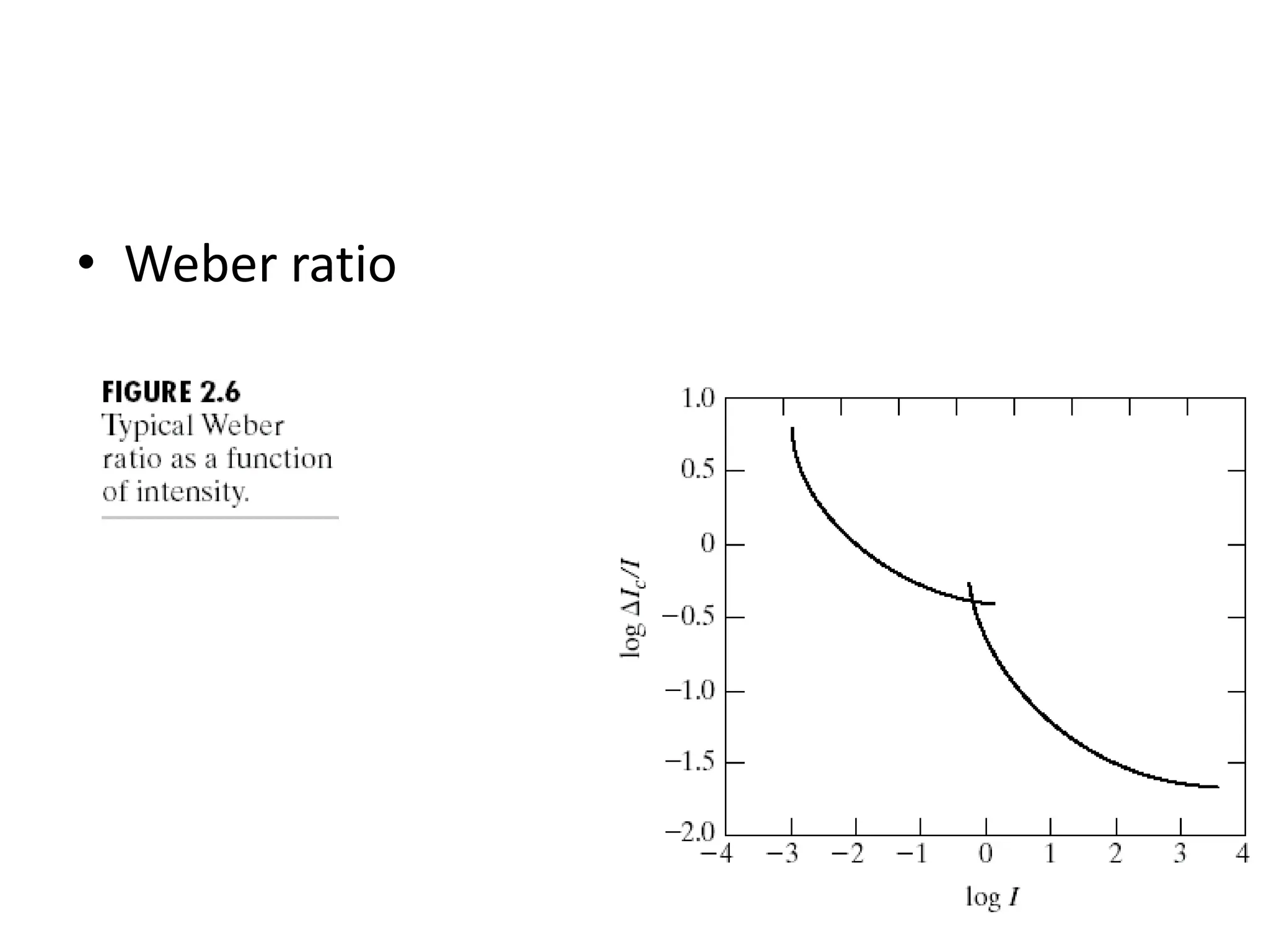
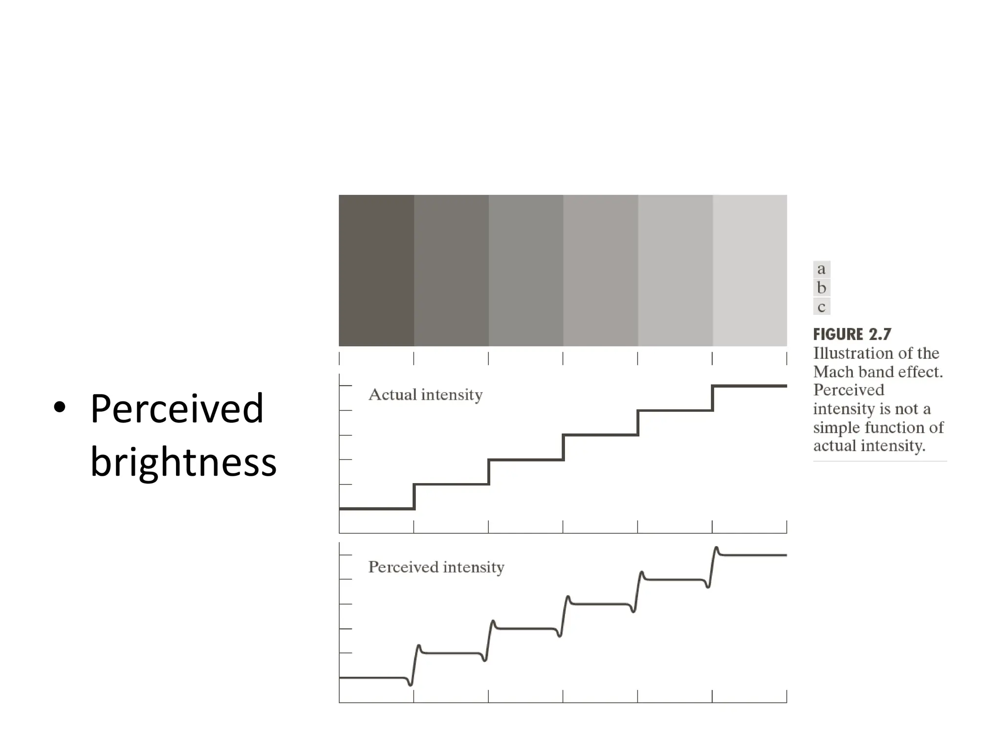
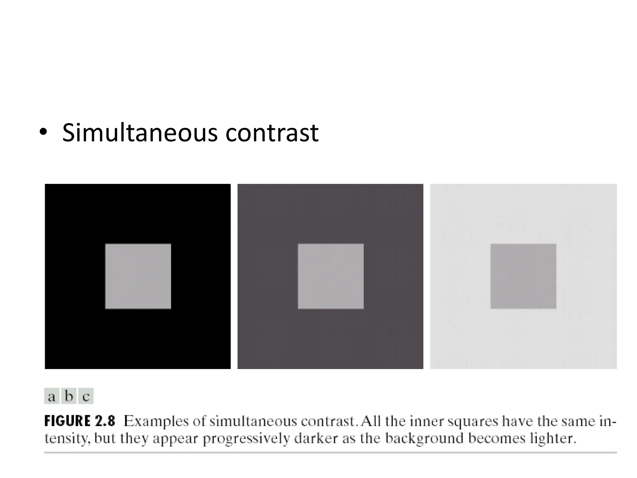
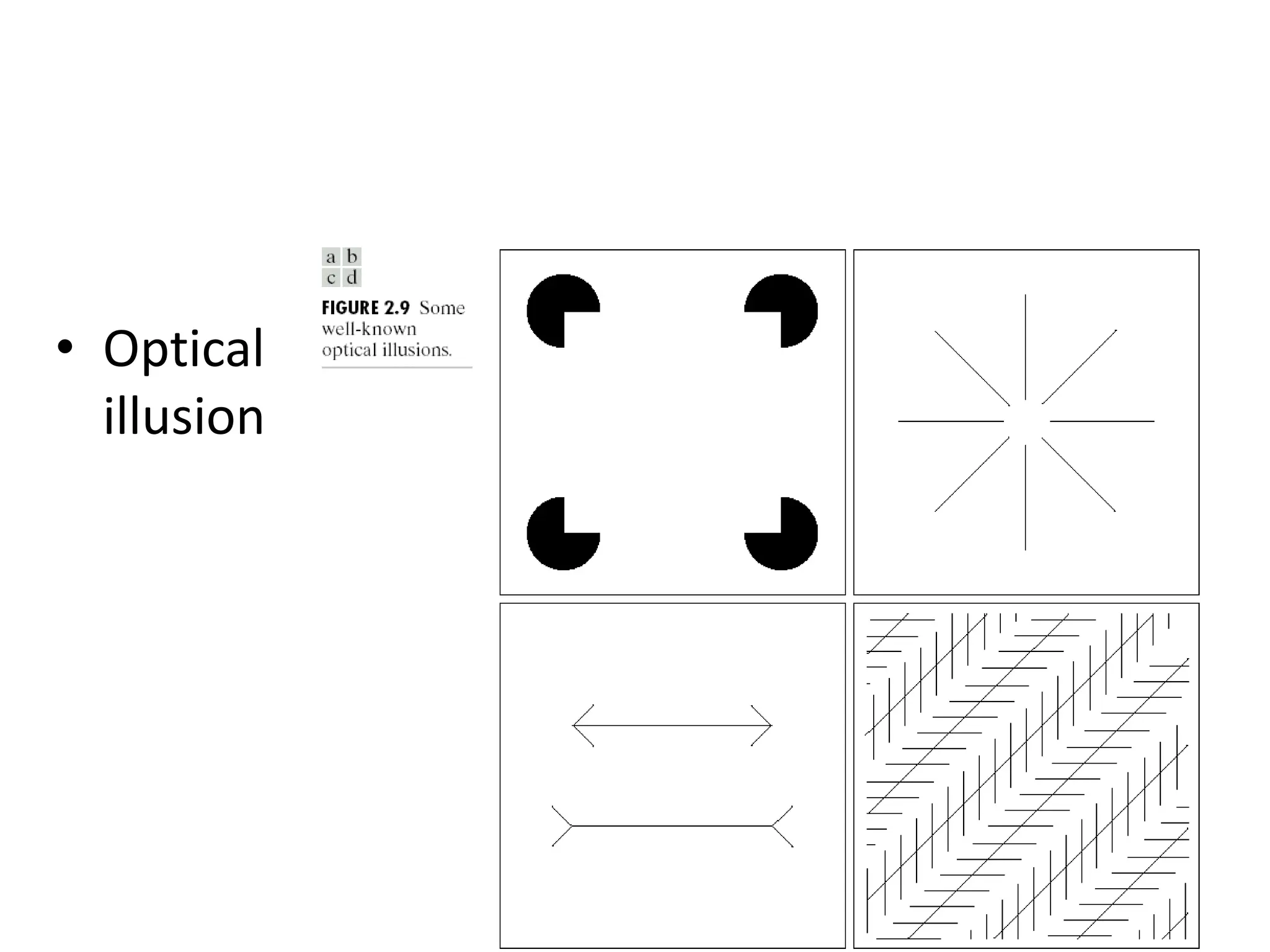
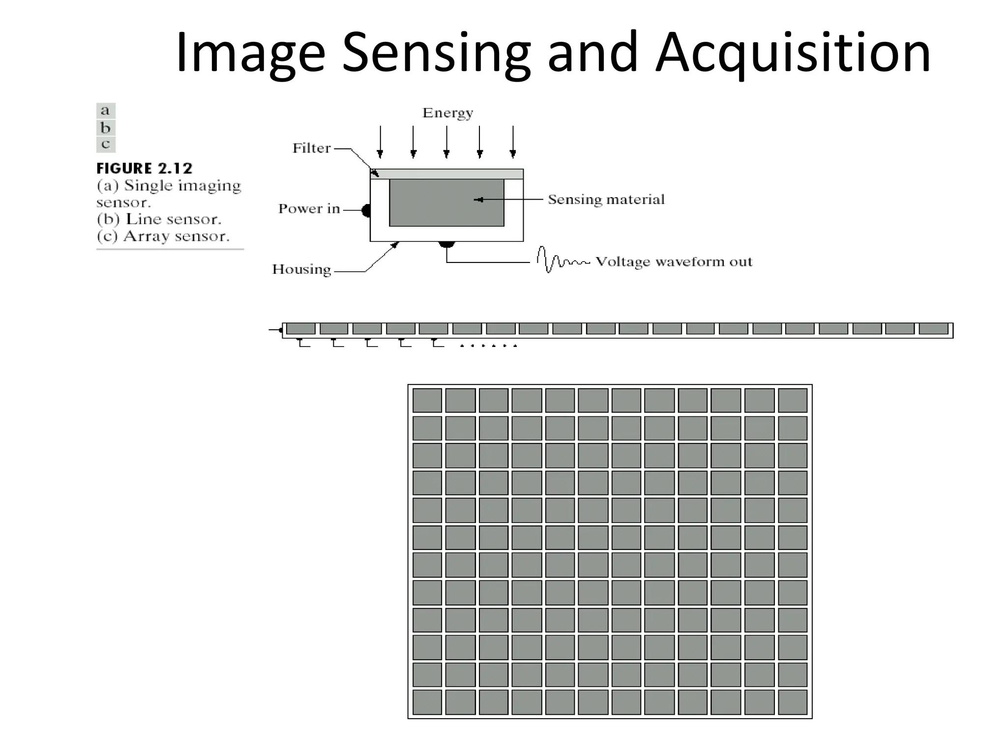
Digital Image Processing Chapter 2: Digital Image Fundamentals
Elements of Visual Perception • Structure of the human eye
• Rods and cones in the retina
• Image formation in the eye
• Brightness adaptation and discrimination
• Brightness discrimination
• Weber ratio
• Perceived brightness
• Simultaneous contrast
• Optical illusion
Light and the Electromagnetic Spectrum
• Wavelength   c   h E 
Image Sensing and Acquisition
• Image acquisition using a single sensor
• Using sensor strips
A simple image formation model
• Illumination and reflectance • Illumination and transmissivity ) , ( ) , ( ) , ( y x r y x i y x f 
Image Sampling and Quantization
Sampling and quantization
• Representing digital images
• Saturation and noise
• Number of storage bits
• Spatial and gray-level resolution
• Subsampled and resampled
• Reducing spatial resolution
• Varying the number of gray levels
• N and k in different-details images
• Isopreference
• Interpolations
• Zooming and shrinking
Some Basic Relationships Between Pixels • Neighbors of a pixel – : 4-neighbors of p , , , : four diagonal neighbors of p , , , : 8-neighbors of p and ) ( 4 p N ) , 1 ( y x  ) 1 , (  y x ) , 1 ( y x  ) 1 , (  y x ) 1 , 1 (   y x ) 1 , 1 (   y x ) 1 , 1 (   y x ) 1 , 1 (   y x ) (p ND ) ( 8 p N ) ( 4 p N ) (p ND
• Adjacency – : The set of gray-level values used to define adjacency – 4-adjacency: Two pixels p and q with values from V are 4-adjacency if q is in the set – 8-adjacency: Two pixels p and q with values from V are 8-adjacency if q is in the set V ) ( 4 p N ) ( 8 p N
– m-adjacency (mixed adjacency): Two pixels p and q with values from V are m-adjacency if • q is in , or • q is in and the set has no pixels whose values are from V ) ( 4 p N ) (p ND ) ( ) ( 4 4 q N p N 
• Subset adjacency – S1 and S2 are adjacent if some pixel in S1 is adjacent to some pixel in S2 • Path – A path from p with coordinates to pixel q with coordinates is a sequence of distinct pixels with coordinates – , ,…, where = , = , and pixels and are adjacent ) , ( y x ) , ( t s ) , ( 0 0 y x ) , ( 1 1 y x ) , ( n n y x ) , ( 0 0 y x ) , ( y x ) , ( n n y x ) , ( t s ) , ( i i y x ) , ( 1 1   i i y x
• Region – We call R a region of the image if R is a connected set • Boundary – The boundary of a region R is the set of pixels in the region that have one or more neighbors that are not in R • Edge – Pixels with derivative values that exceed a preset threshold
• Distance measures – Euclidean distance – City-block distance – Chessboard distance 2 1 2 2 ] ) ( ) [( ) , ( t y s x q p De     | ) ( | | ) ( | ) , ( 4 t y s x q p D     |) ) ( | |, ) ( max(| ) , ( 8 t y s x q p D   
m D  distance: The shortest m-path between the points
An Introduction to the Mathematical Tools Used in Digital Image Processing • Linear operation – H is said to be a linear operator if, for any two images f and g and any two scalars a and b, ) ( ) ( ) ( g bH f aH bg af H   
• Arithmetic operations – Addition
• Arithmetic operations – Subtraction
– Digital subtraction angiography
– Shading correction
• Image multiplication
• Set operations
• Complements
• Logical operations
• Single-pixel operations
• Neighborhood operations
• Affine transformations
• Inverse mapping
• Registration
• Vector operations
• Image transforms
• Fourier transform
• Probabilistic methods

digital image processing chapter two, fundamentals