unit-4 data structure notesfor computer science

unit-4 data structure notesfor computer science

• 1.
  U N IT – 4 • Greedy Method • The General Method • Optimal Storage on Tapes • Knapsack Problem • Job Sequencing with Deadlines • Optimal Merge Patterns.
• 2.
   This isdone by considering the inputs in an order determined by some selection procedure.  If the inclusion of the next input into the partially constructed optimal solution will result in an infeasible solution, then this input is not added to the partial solution. Otherwise, it is added.  The selection procedure itself is based on some optimization measure. This measure may be the objective function. In fact, several different optimization measures may be plausible for a given problem.  Most of these, however, will result in algorithms that generate suboptimal solutions. This version of the greedy technique is called the subset paradigm. GREEDY METHOD
• 3.
   The greedymethod is the most straightforward design technique. It can be applied to a wide variety of problems. Most of these problems have n inputs and require us to obtain a subset that satisfies some constraints.  Any subset that satisfies these constraints is called a feasible solution.  We need to find a feasible solution that either maximizes or minimizes a given objective function. A feasible solution that does this is called an optimal solution. The greedy method suggests that one can devise an algorithm that works in stages, considering one input at a time. GREEDY METHOD RULES
• 4.
   The functionSelect selects an input from a[] and removes it. The selected input's value is assigned to x.  Feasible is a Boolean-valued function that determines whether x can be included into the solution vector.  The function Union combines x with the solution and updates the objective function.  The function Greedy describes the essential way that a greedy algorithm will look, once a particular problem is chosen and the functions Select, Feasible, and Union are properly implemented. GREEDY METHOD FUNCTION
• 5.
  1 Algorithm Greedy(a,n) 2/ / a[l : n] contains the n inputs. 3 { 4 solution := 0; / / Initialize the solution. 5 for i := 1 to n do 6 { 7 x := Select(a); 8 if Feasible(solution, x) then 9solution:= Union(solution, x); 10 } 11 return solution; 12 } GREEDY ALGORITHM
• 6.
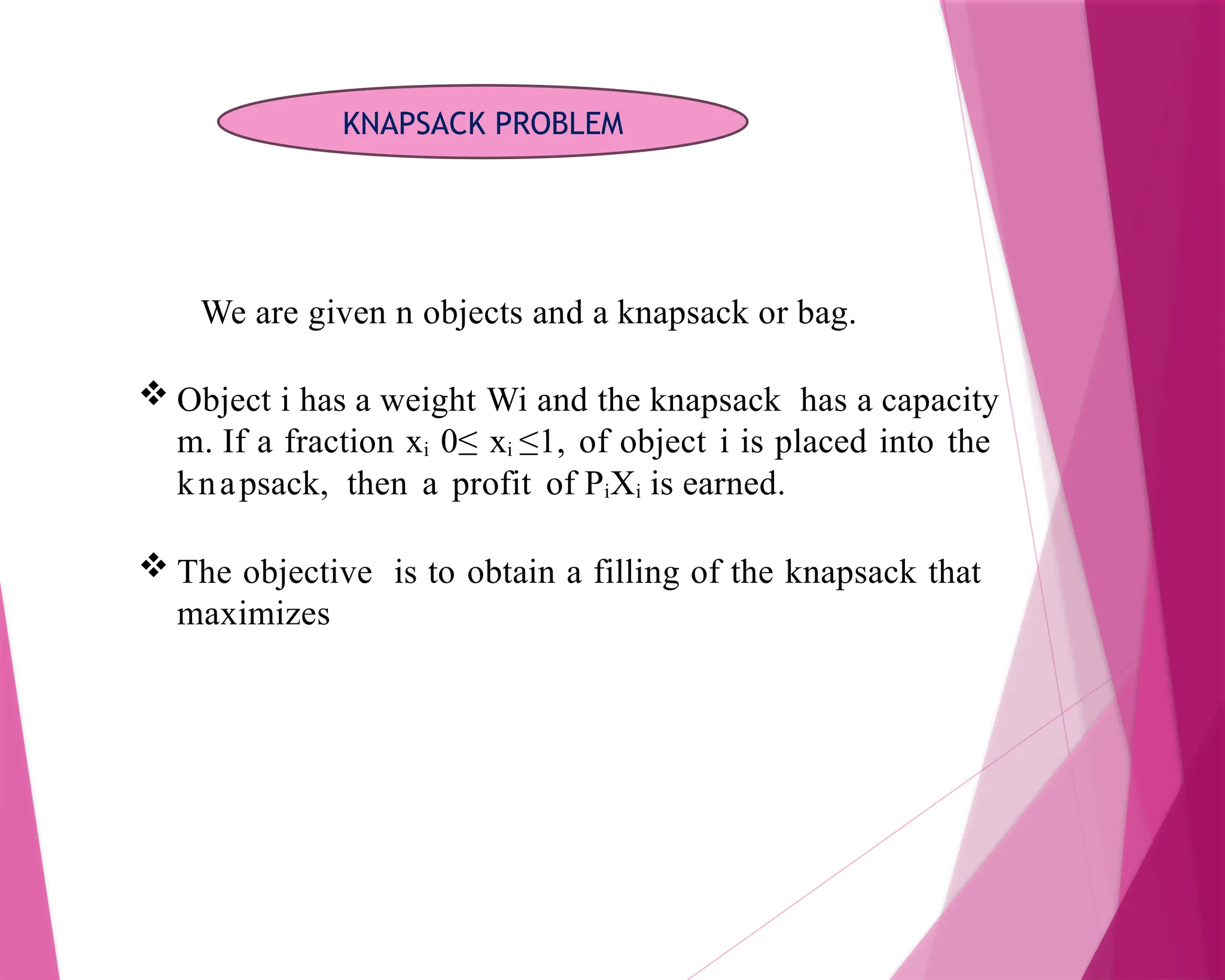
  We are givenn objects and a knapsack or bag.  Object i has a weight Wi and the knapsack has a capacity m. If a fraction xi 0≤ xi ≤1, of object i is placed into the knapsack, then a profit of PiXi is earned.  The objective is to obtain a filling of the knapsack that maximizes KNAPSACK PROBLEM
• 7.
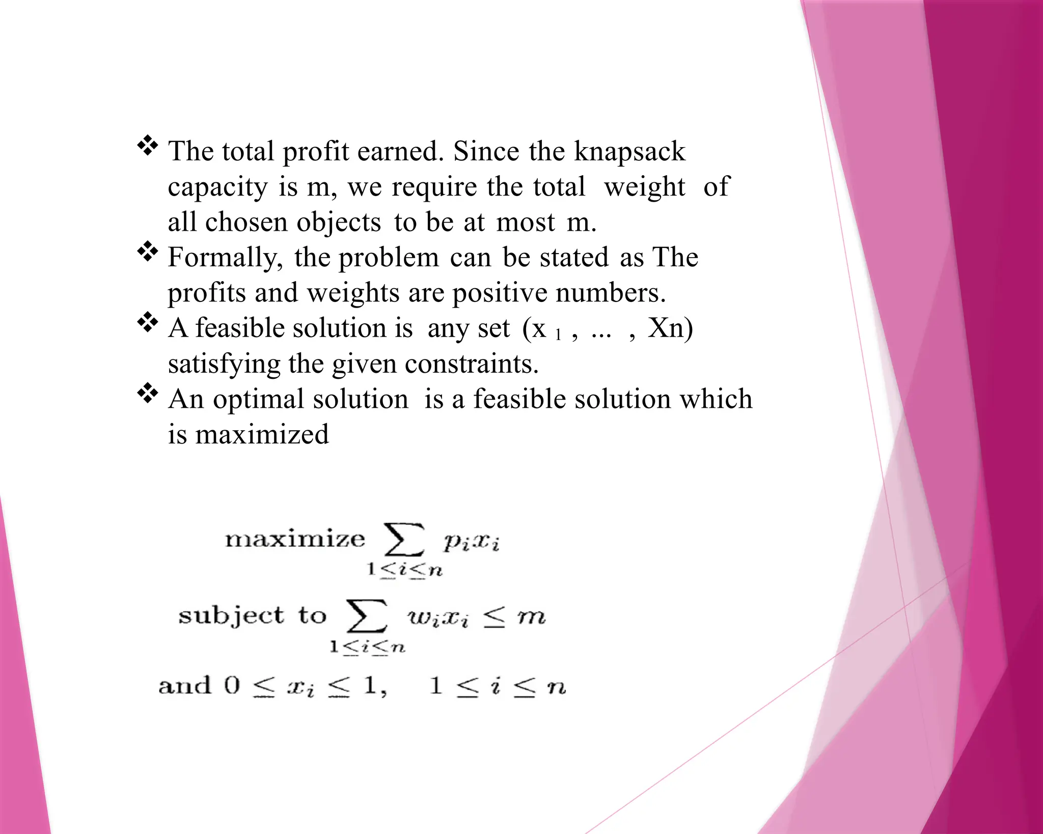
   The totalprofit earned. Since the knapsack capacity is m, we require the total weight of all chosen objects to be at most m.  Formally, the problem can be stated as The profits and weights are positive numbers.  A feasible solution is any set (x 1 , ... , Xn) satisfying the given constraints.  An optimal solution is a feasible solution which is maximized
• 8.
  Algorithm GreedyKnapsack (m,n) { for i 1  to n do x[i] = 0.0; U = m; for i 1  to n do { if(w[i] > U) then break; x[i] = 1.0; U = U – w[i]; } if (i<=m) x[i] = U/w[i]; } KNAPSACK ALGORITHM
• 9.
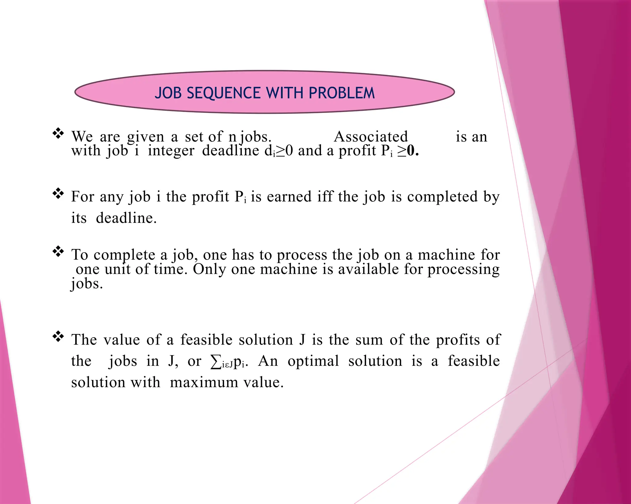
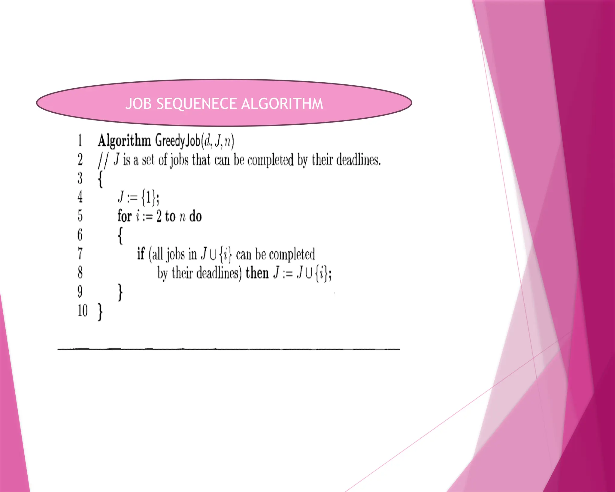
   We aregiven a set of n jobs. Associated is an with job i integer deadline di≥0 and a profit Pi ≥0.  For any job i the profit Pi is earned iff the job is completed by its deadline.  To complete a job, one has to process the job on a machine for one unit of time. Only one machine is available for processing jobs.  The value of a feasible solution J is the sum of the profits of the jobs in J, or ∑iεJpi. An optimal solution is a feasible solution with maximum value. JOB SEQUENCE WITH PROBLEM
• 10.
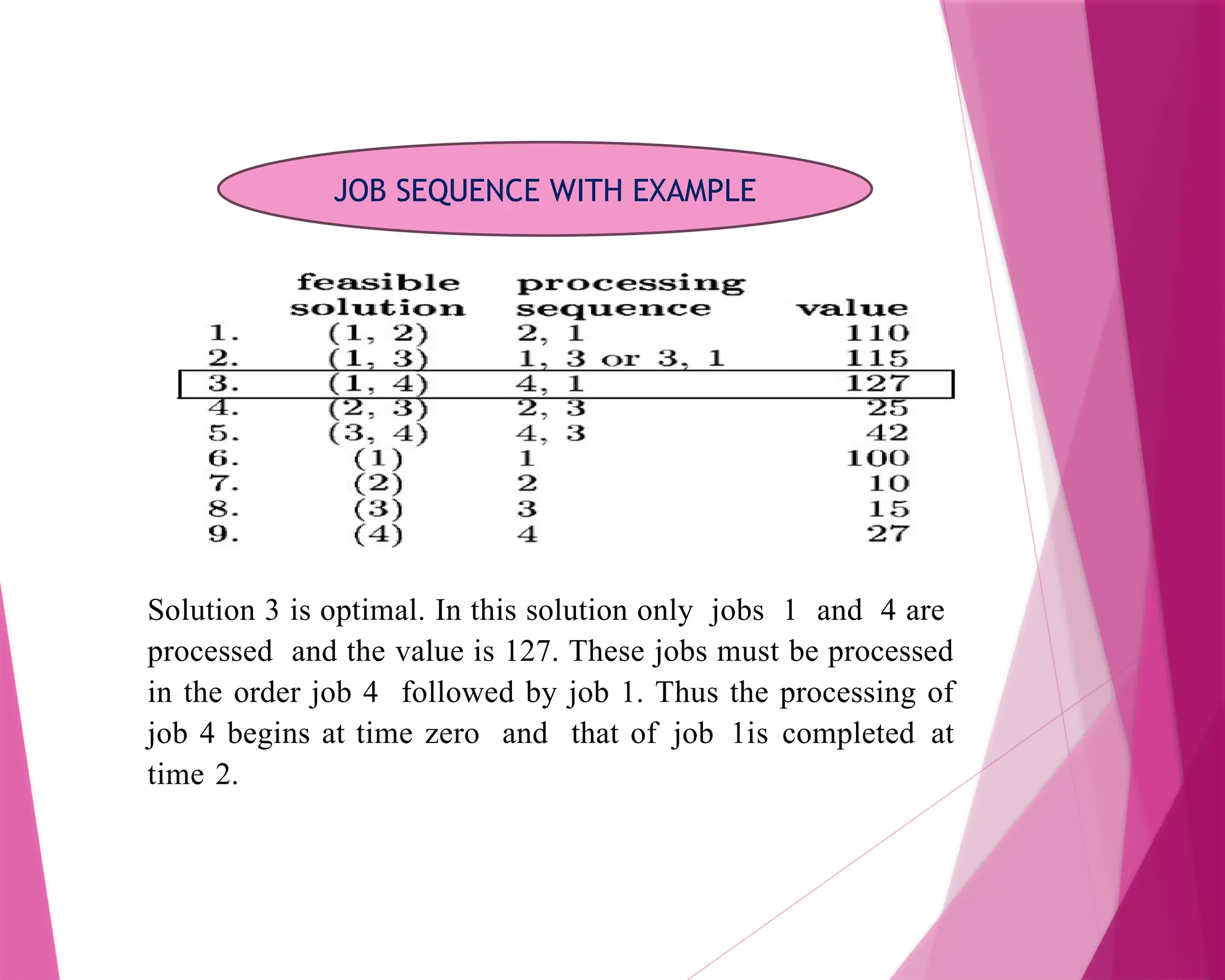
  Solution 3 isoptimal. In this solution only jobs 1 and 4 are processed and the value is 127. These jobs must be processed in the order job 4 followed by job 1. Thus the processing of job 4 begins at time zero and that of job 1is completed at time 2. JOB SEQUENCE WITH EXAMPLE
• 11.
  JOB SEQUENECE ALGORITHM
• 12.
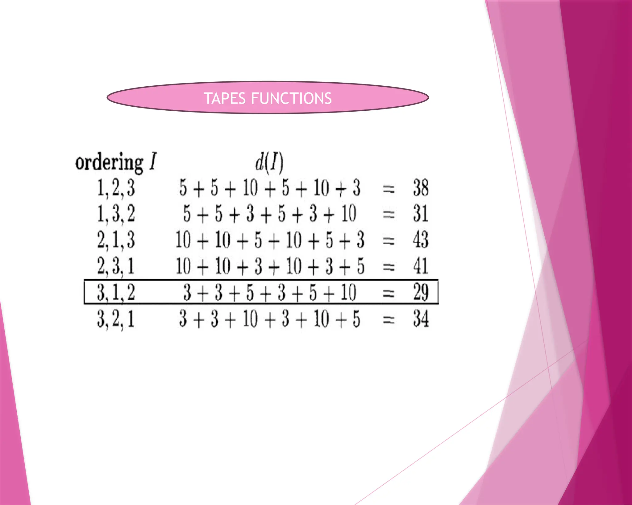
   We assumethat whenever a program is to be retrieved from this tape, the tape is initially positioned at the front.  Hence, if the programs are stored in the order I= i1, i2, ... , in, the time tj needed to retrieve program ij is proportional to ∑l≤k≤j lik.  If all programs are retrieved equally often, then the expected or mean retrieval time (MRT) is (1/n) ∑l≤j≤n tj.  In the optimal storage on tape problem, we are required to find a permutation for the n programs so that when they are stored on the tape in this order the MRT is minimized.  This problem fits the ordering paradigm. Minimizing the MRT is equivalent to minimizing d(I) =∑l≤j≤n∑l≤k≤j lik. OPTIMAL STORAGE ON TAPES
• 13.
  TAPES FUNCTIONS
• 14.
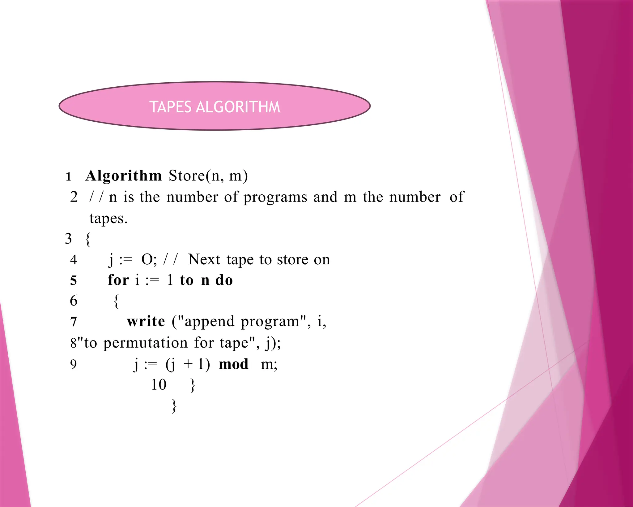
  1 Algorithm Store(n,m) 2 / / n is the number of programs and m the number of tapes. 3 { 4 j := O; / / Next tape to store on 5 for i := 1 to n do 6 { 7 write ("append program", i, 8"to permutation for tape", j); 9 j := (j + 1) mod m; 10 } } TAPES ALGORITHM
• 15.
   The optimalmerge pattern problem describes that there two sorted files containing n and m records respectively could be merged together to obtain one sorted file in time O(n +m).  When more than two sorted files are to be merged together, the merge can be accomplished by repeatedly merging sorted files in pairs.  Thus, if files x1 , x2, x3 and x4 are to be merged, we could first merge x1 and x2 to get a file y1. Then we could merge y1 and x3 to gety2. Finally, wecould merge y2 and x4 to get the desired sorted file. OPTIMAL MERGE PATTERNS
• 16.
   Alternatively, wecould first merge x1 and x2 getting yl, then merge x3 and x4 and get y2, and finally merge y1 and y2 and get the desired sorted file.  Given n sorted files, there are many ways in which to pairwise merge them into a single sorted file.  Different pairings require differing amounts of computing time. The problem we address ourselves to now is that of determining an optimal way to pairwise merge n sorted files.
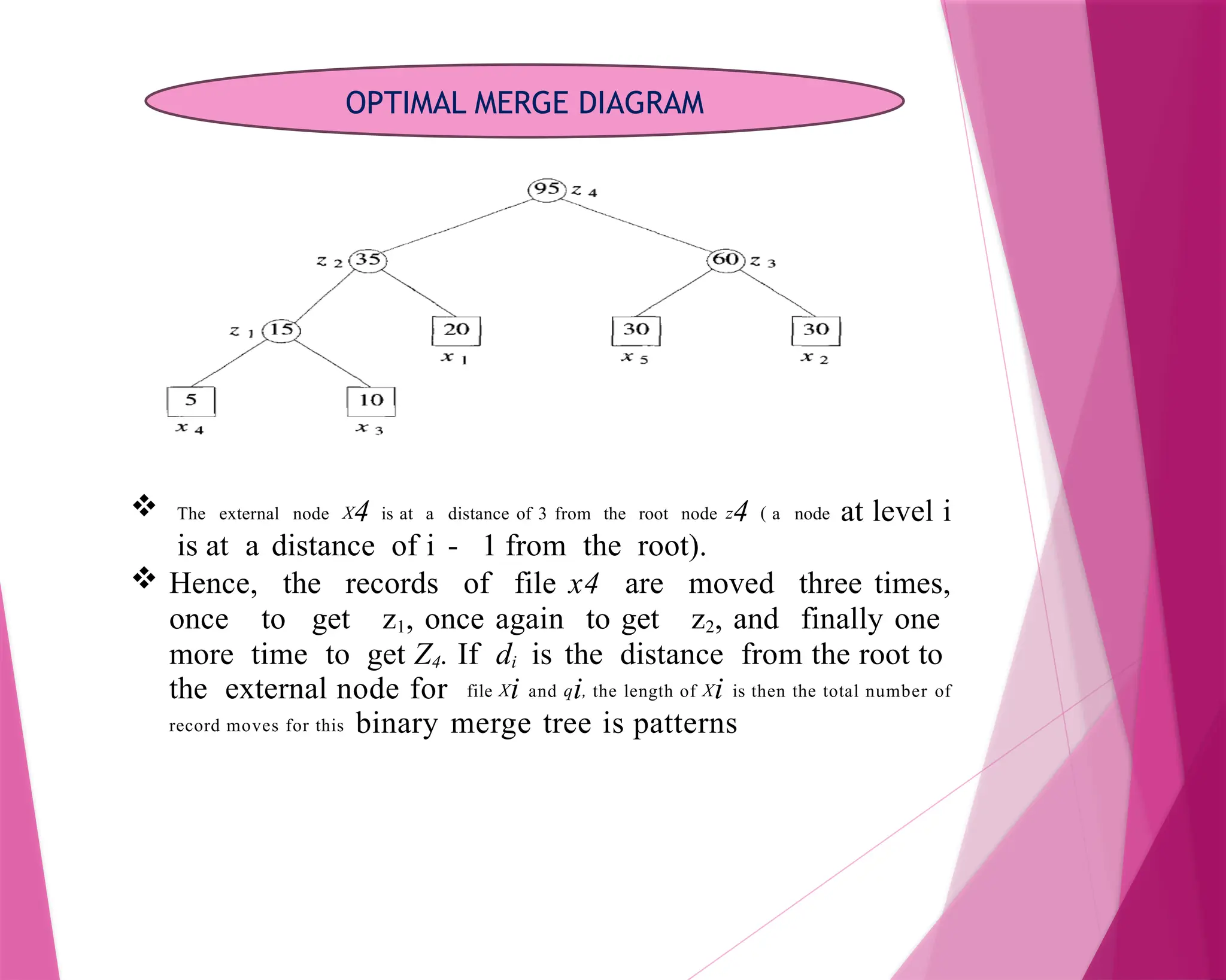
• 17.
   The externalnode X4 is at a distance of 3 from the root node z4 ( a node at level i is at a distance of i - 1 from the root).  Hence, the records of file x4 are moved three times, once to get z1, once again to get z2, and finally one more time to get Z4. If di is the distance from the root to the external node for file Xi and qi, the length of Xi is then the total number of record moves for this binary merge tree is patterns OPTIMAL MERGE DIAGRAM