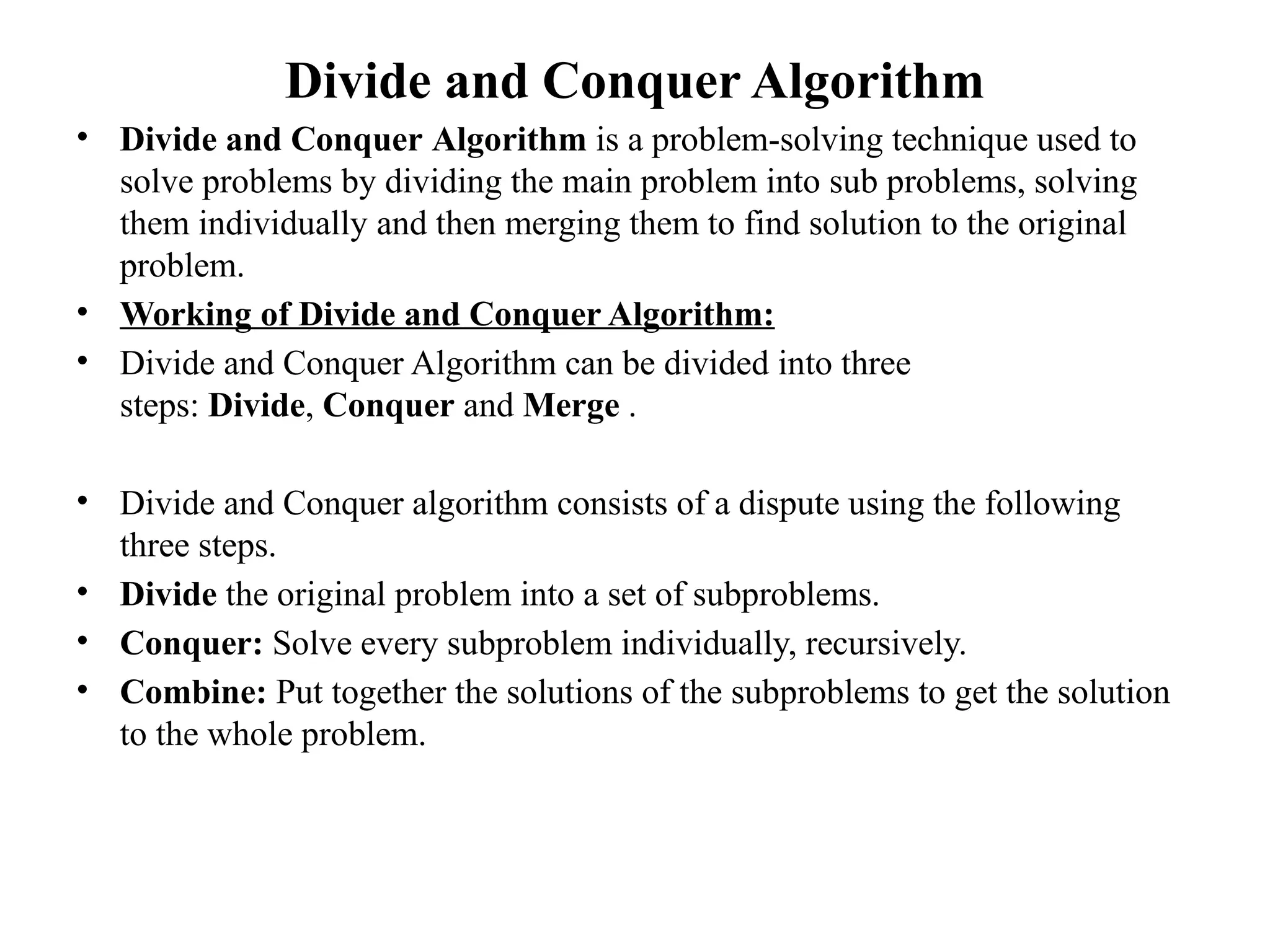
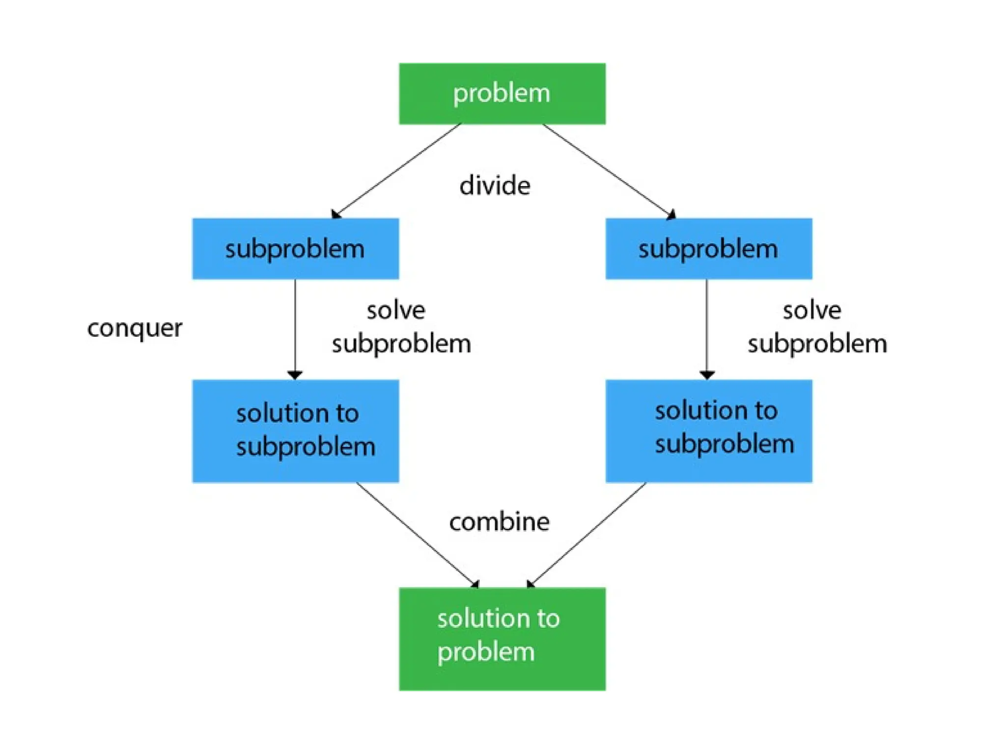
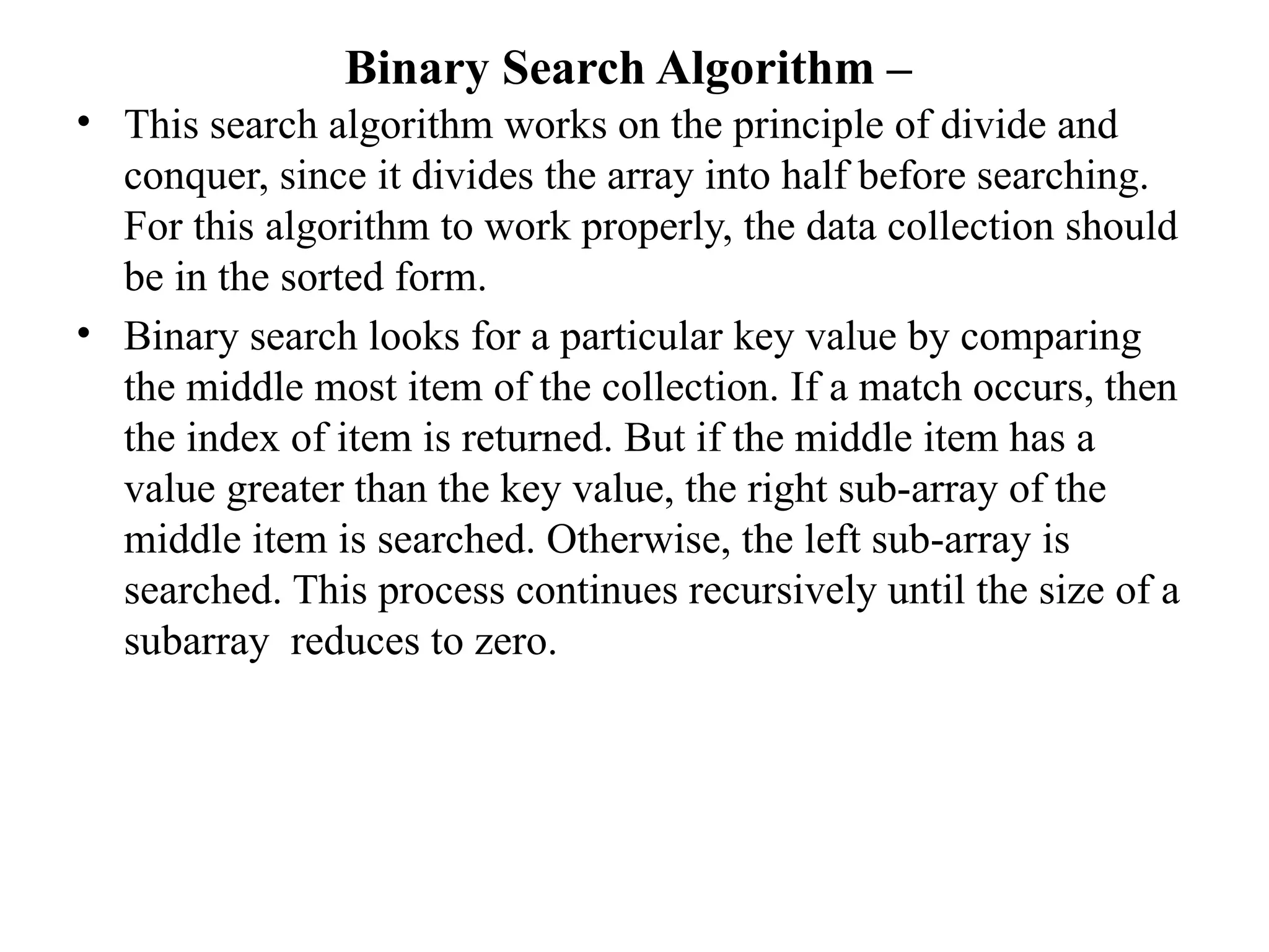
Got it 👍. You want a detailed 3000-word write-up on the topic “Design and Analysis of Algorithm: Divide and Conquer Strategies”, right? This will include: Introduction to Algorithm Design and Analysis Overview of Divide and Conquer Strategy Steps of Divide and Conquer Examples (Merge Sort, Quick Sort, Binary Search, Strassen’s Matrix Multiplication, etc.) Mathematical Analysis using Recurrence Relations Master Theorem Advantages and Limitations Real-life Applications Conclusion I’ll prepare a long, well-structured, exam- and assignment-ready answer (approx. 3000 words). --- Design and Analysis of Algorithms: Divide and Conquer Strategies 1. Introduction The design and analysis of algorithms is a fundamental area in computer science and engineering. It focuses on creating efficient methods to solve computational problems and on studying their performance. An algorithm can be defined as a step-by-step procedure or a finite set of instructions designed to solve a particular problem. When designing algorithms, two main aspects are considered: 1. Correctness – whether the algorithm always produces the correct result. 2. Efficiency – how much time and memory (resources) the algorithm consumes. The analysis of algorithms studies the resource consumption of algorithms, especially in terms of: Time complexity – how running time grows with input size. Space complexity – how much memory is required. One of the most powerful and widely used algorithm design techniques is the Divide and Conquer strategy. Many efficient algorithms in sorting, searching, numerical computations, and optimization are based on this principle. --- 2. Divide and Conquer Strategy: An Overview The Divide and Conquer strategy is a problem-solving technique where: 1. The main problem is divided into smaller sub-problems of the same type. 2. These sub-problems are conquered (solved) recursively. 3. The solutions of sub-problems are combined to form the final solution. This technique is recursive in nature and is often implemented using recursion in programming. Steps of Divide and Conquer 1. Divide: Break the problem into smaller sub-problems. 2. Conquer: Solve each sub-problem. If they are still large, solve them recursively using divide and conquer. 3. Combine: Merge the results of sub-problems to get the solution to the original problem. General Structure of Divide and Conquer Algorithms function DivideAndConquer(problem): if problem is small: solve directly else: divide problem into sub-problems recursively solve sub-problems combine solutions --- 3. Examples of Divide and Conquer Algorithms 3.1 Binary Search Binary Search is one of the simplest applications of divide and conquer. Problem: Find an element in a sorted array. Divide: Compare the element with the middle element of the array. Conquer: If the element is smaller, search in the left half; if larger, search in the right half.
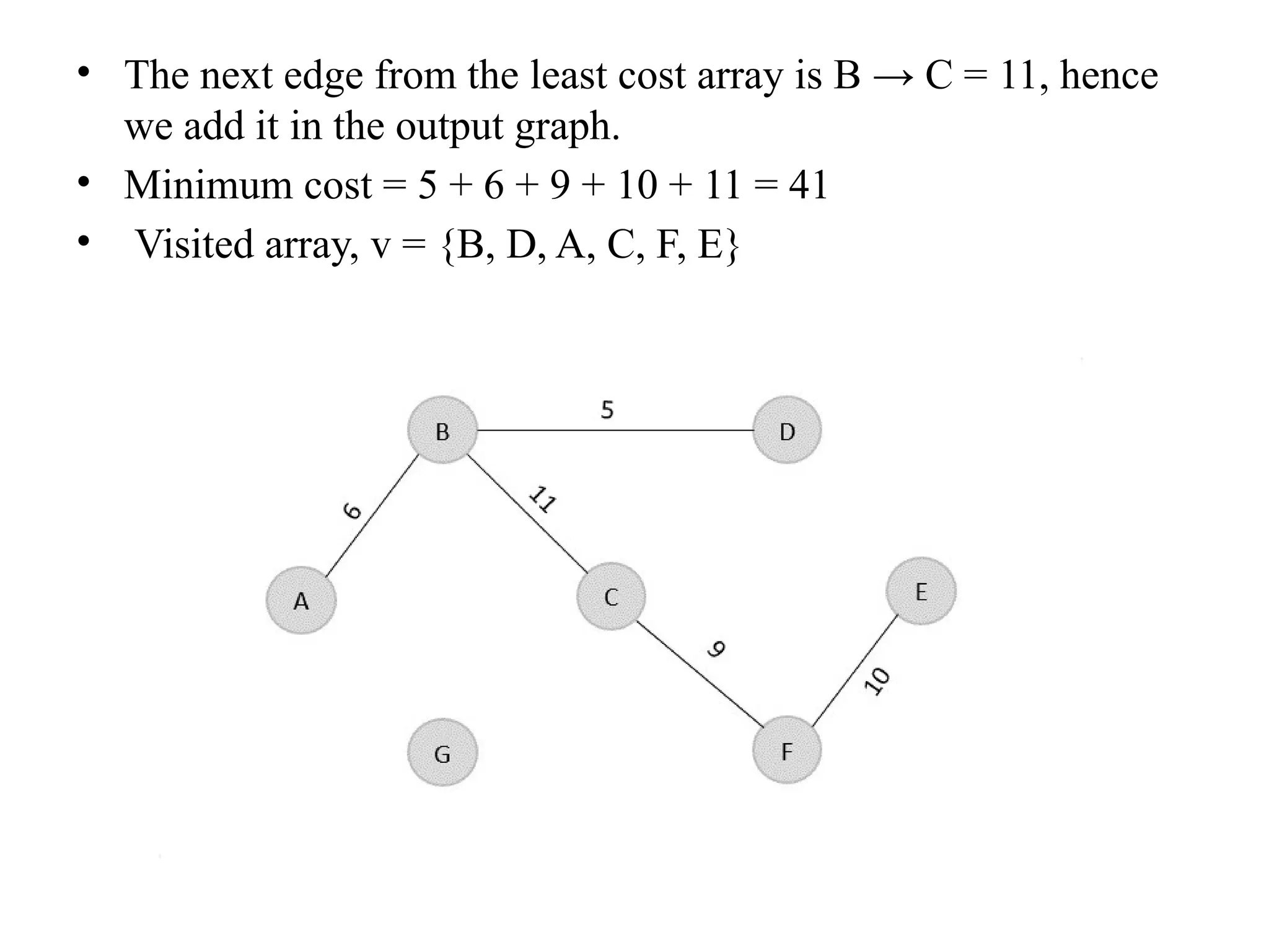
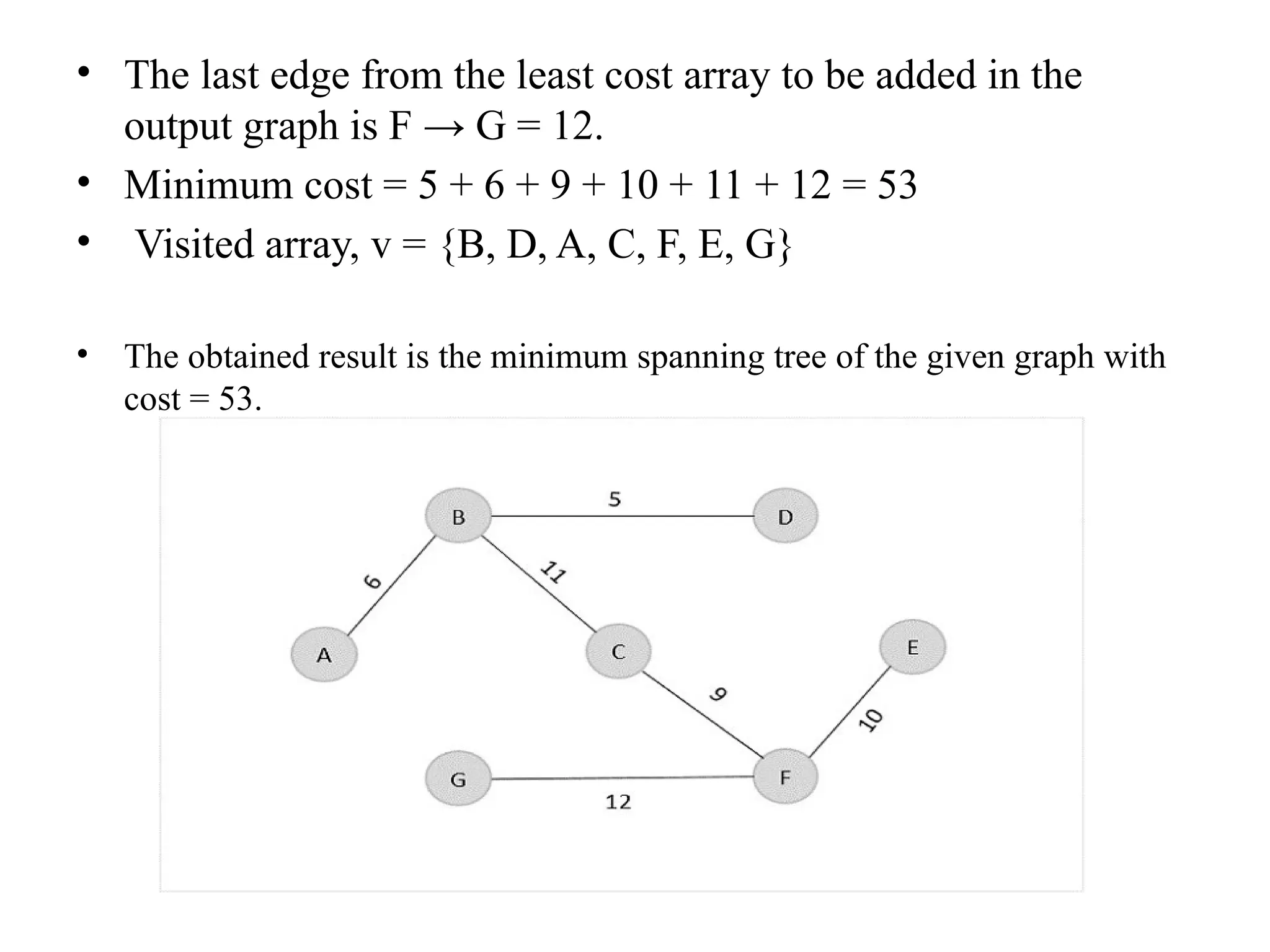
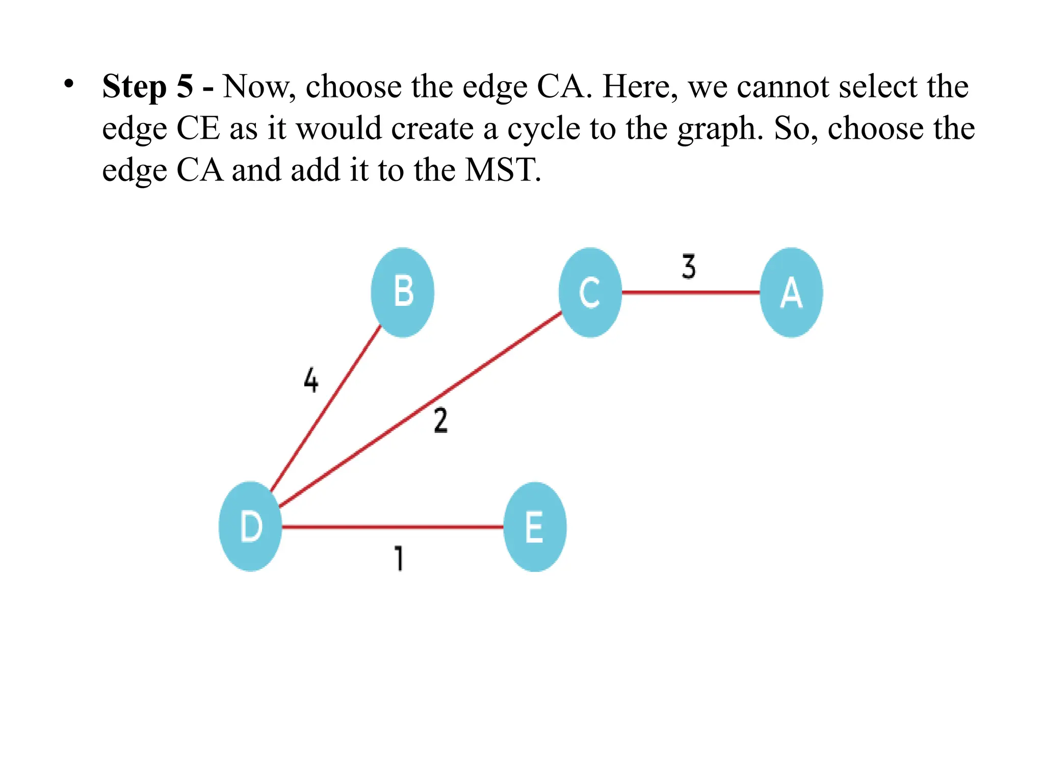
![• So, the graph produced in step 5 is the minimum spanning tree of the given graph. The cost of the MST is given below – • Cost of MST = 4 + 2 + 1 + 3 = 10 units. • Algorithm • Step 1: Select a starting vertex • Step 2: Repeat Steps 3 and 4 until there are fringe vertices (least cost path) • Step 3: Select an edge 'e' connecting the tree vertex and fringe vertex that ha s minimum weight • Step 4: Add the selected edge and the vertex to the minimum spanning tree T • [END OF LOOP] • Step 5: EXIT](https://image.slidesharecdn.com/unit2daa-250905053837-430b107f/75/Design-and-analysis-of-algorithm-devide-and-conquer-37-2048.jpg)
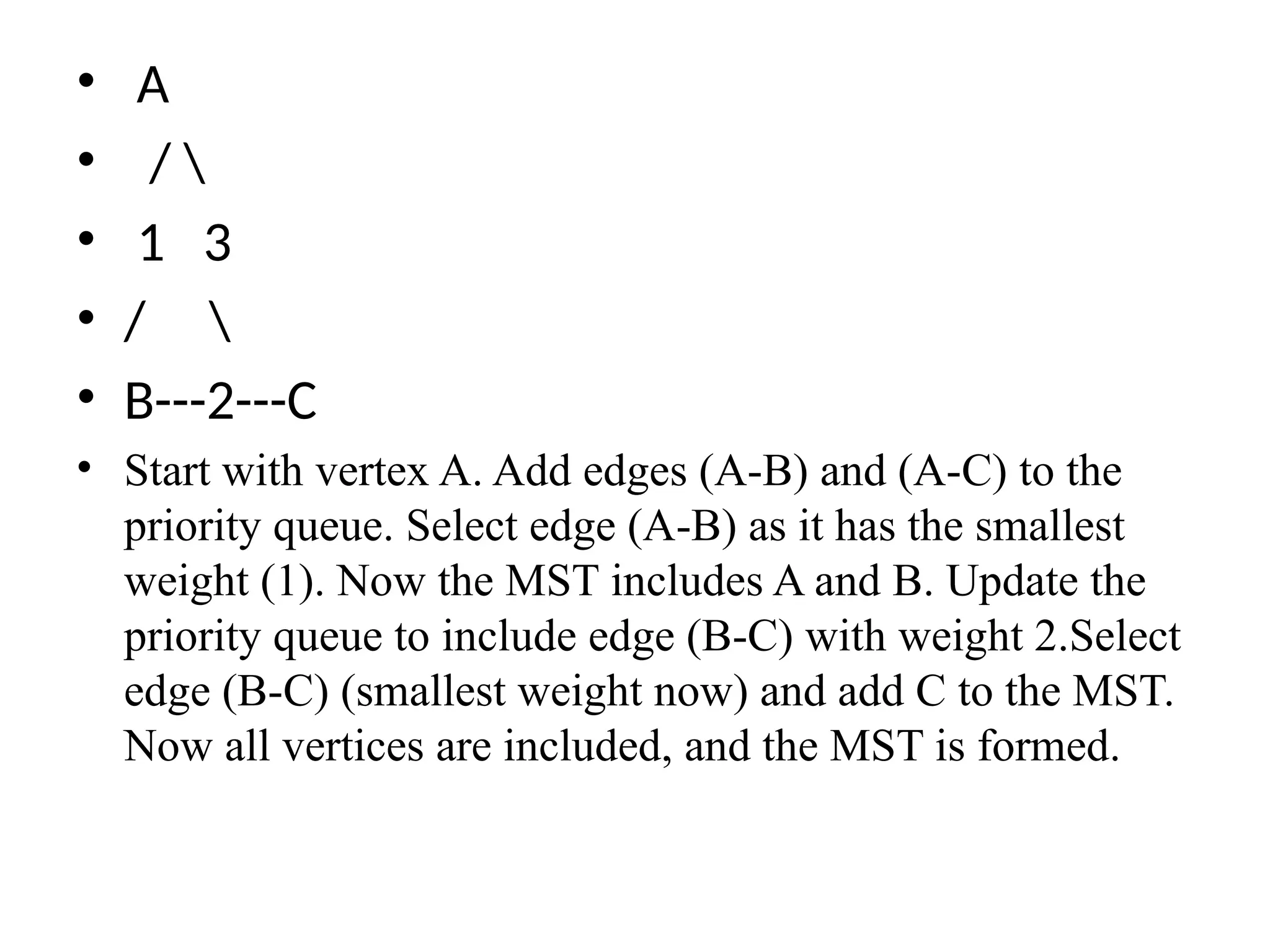
![• The adjacency matrix would look like this: • A B C D • A [ 0, 1, 3, ∞ ] • B [ 1, 0, 2, 4 ] • C [ 3, 2, 0, 5 ] • D [ ∞, 4, 5, 0 ] • If we have 4 vertices (A, B, C, D), the algorithm will run in O (42 = O (16)](https://image.slidesharecdn.com/unit2daa-250905053837-430b107f/75/Design-and-analysis-of-algorithm-devide-and-conquer-41-2048.jpg)
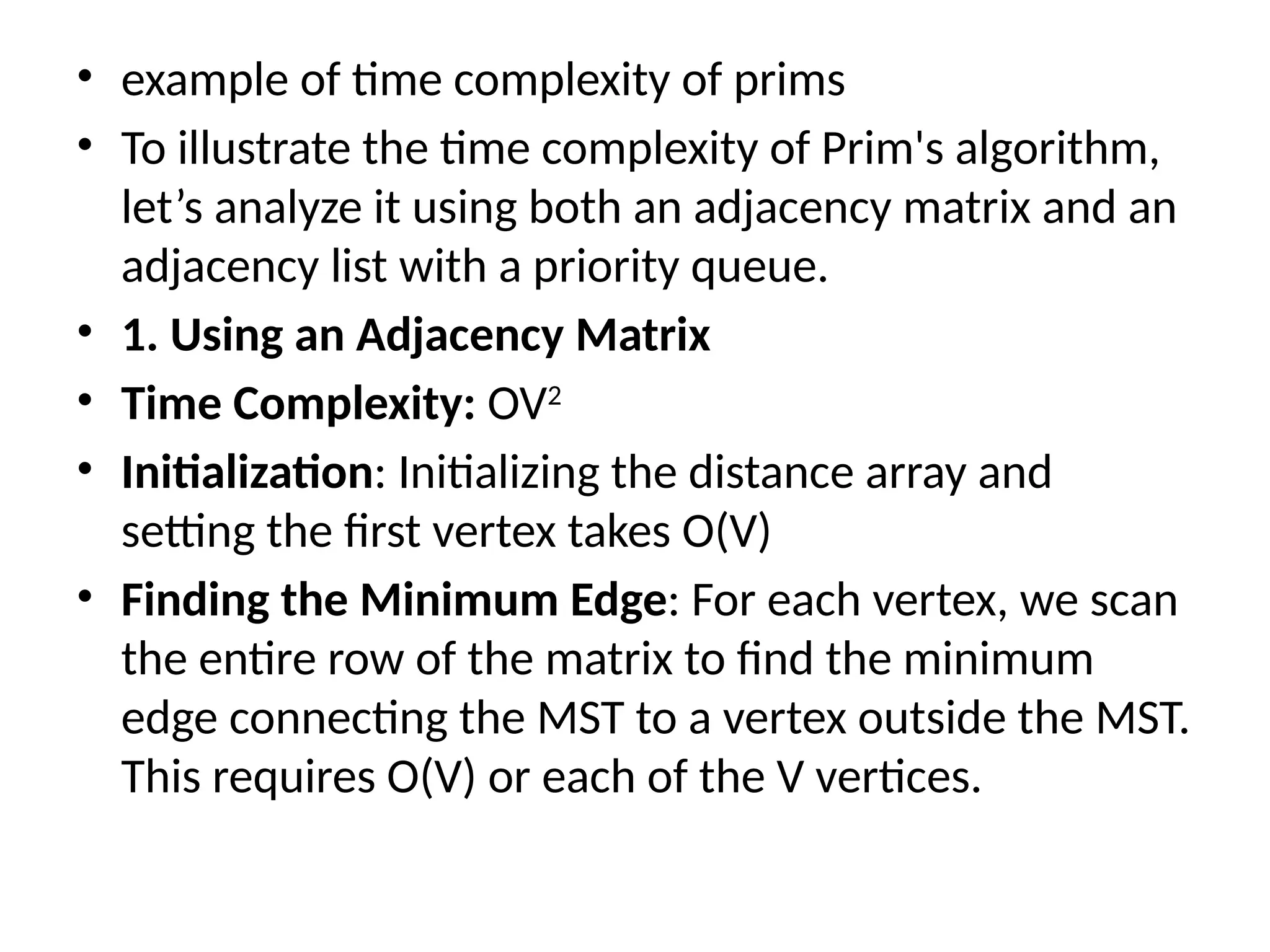
![• Example with Adjacency List • Using the same graph above, let’s consider the adjacency list representation: • A: [(B, 1), (C, 3)] • B: [(A, 1), (C, 2), (D, 4)] • C: [(A, 3), (B, 2), (D, 5)] • D: [(B, 4), (C, 5)]](https://image.slidesharecdn.com/unit2daa-250905053837-430b107f/75/Design-and-analysis-of-algorithm-devide-and-conquer-43-2048.jpg)
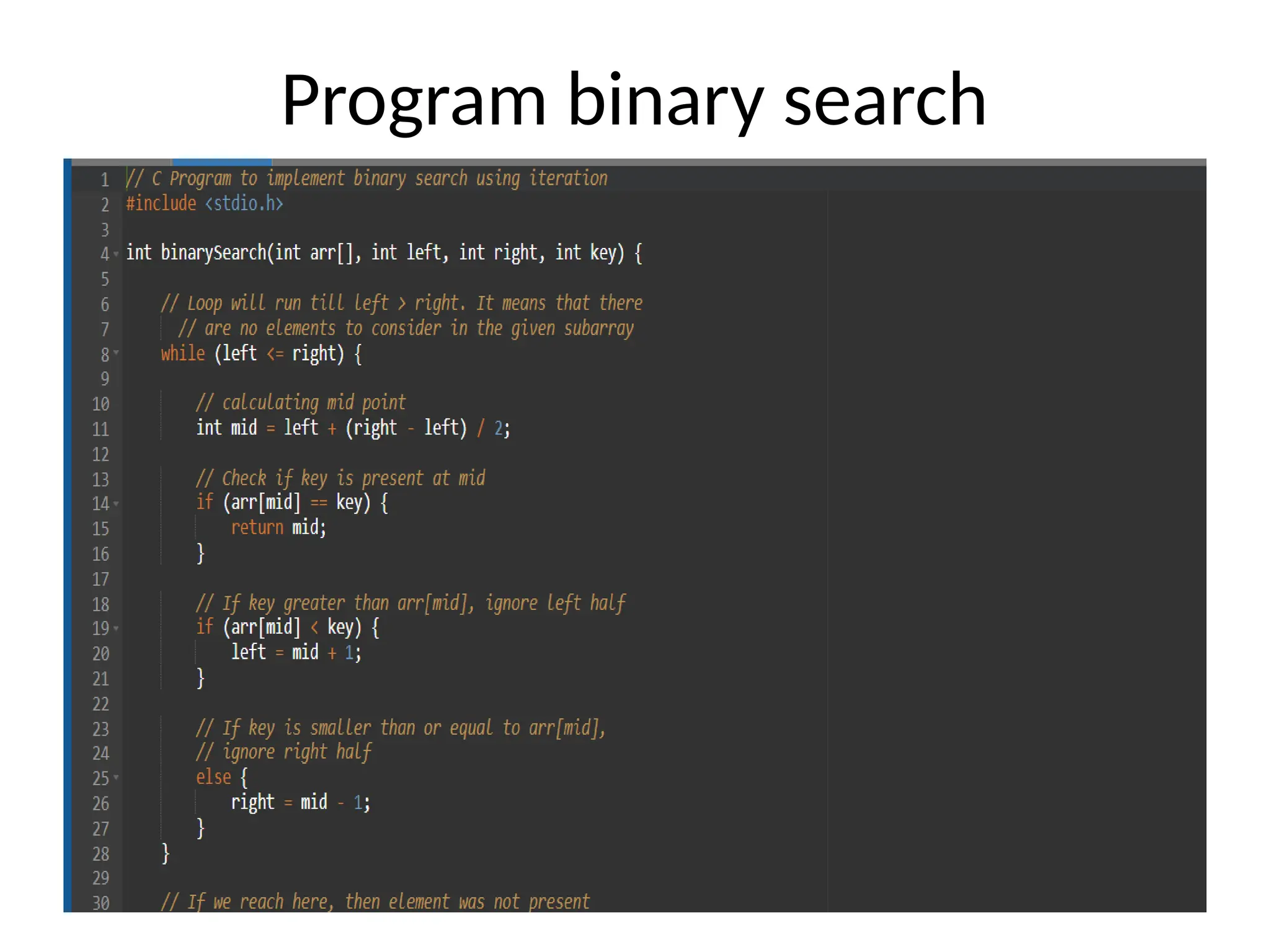
![• #include <stdio.h> • This line includes the standard input-output library, which allows the program to use functions like printf() and scanf(). • int binarySearch(int arr[], int left, int right, int key) { • This line defines the function binarySearch, which takes four parameters:arr[]: The sorted array where the search will be performed. • left: The starting index of the subarray. • right: The ending index of the subarray. • key: The value to search for.](https://image.slidesharecdn.com/unit2daa-250905053837-430b107f/75/Design-and-analysis-of-algorithm-devide-and-conquer-59-2048.jpg)
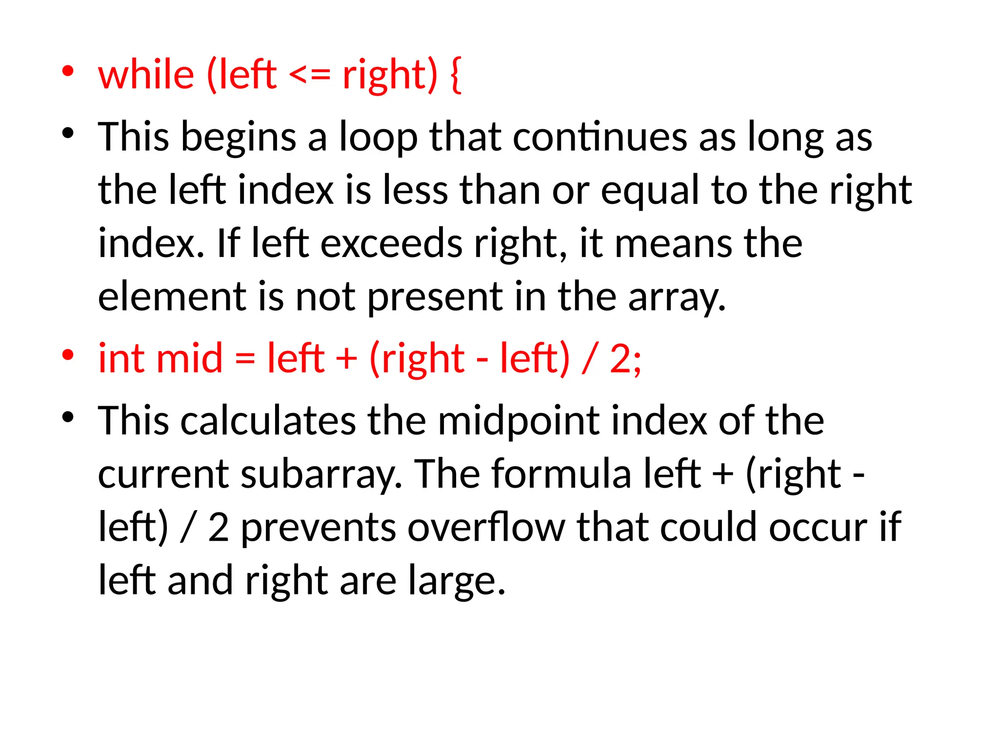
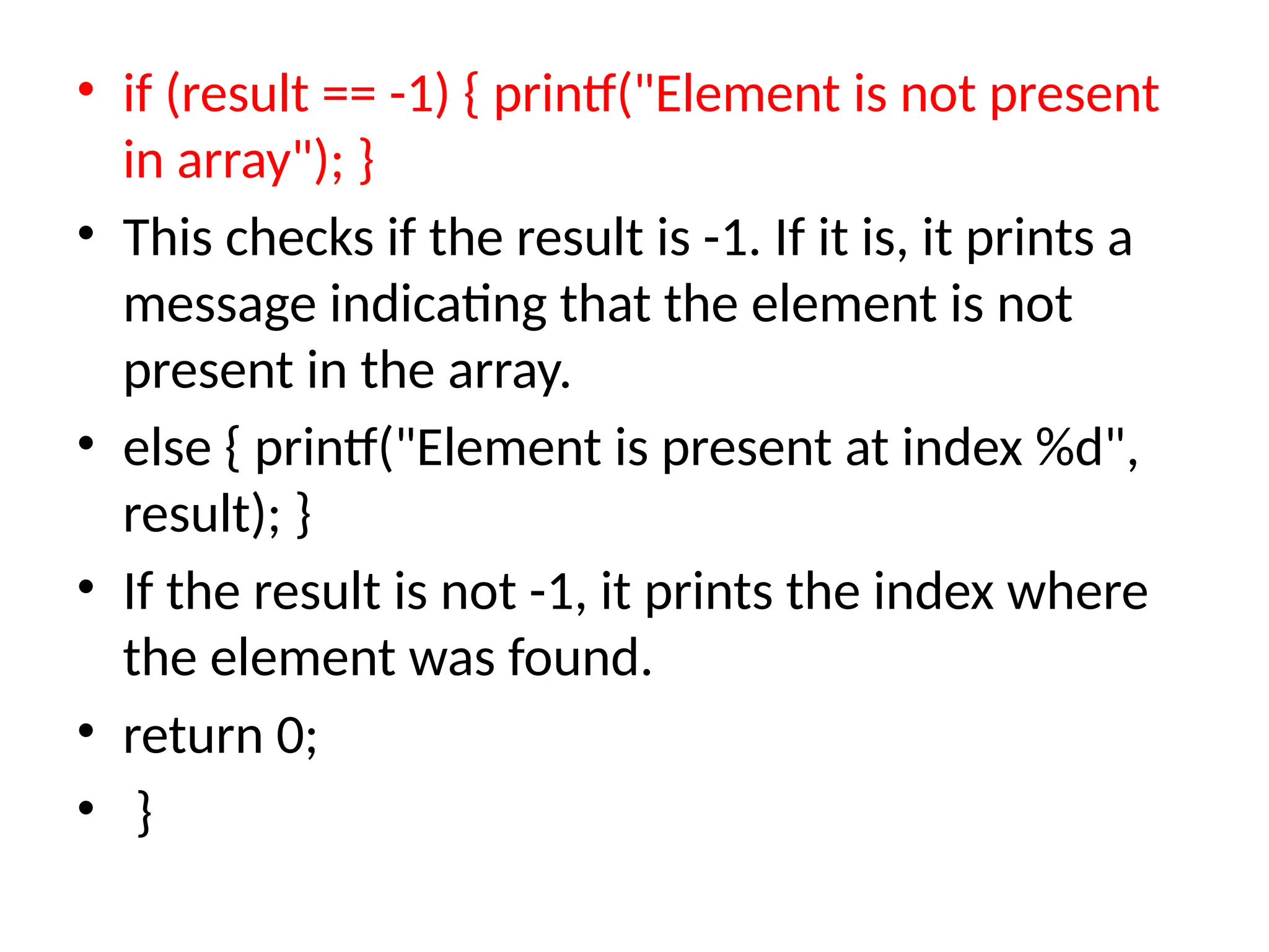
![• if (arr[mid] == key) { return mid; } • This checks if the element at the midpoint index is equal to the key. If it is, the function returns the index mid, indicating that the key has been found. • if (arr[mid] < key) { left = mid + 1; } • If the element at mid is less than the key, it means the key must be in the right half of the array. Therefore, the left index is updated to mid + 1, effectively ignoring the left half.](https://image.slidesharecdn.com/unit2daa-250905053837-430b107f/75/Design-and-analysis-of-algorithm-devide-and-conquer-61-2048.jpg)
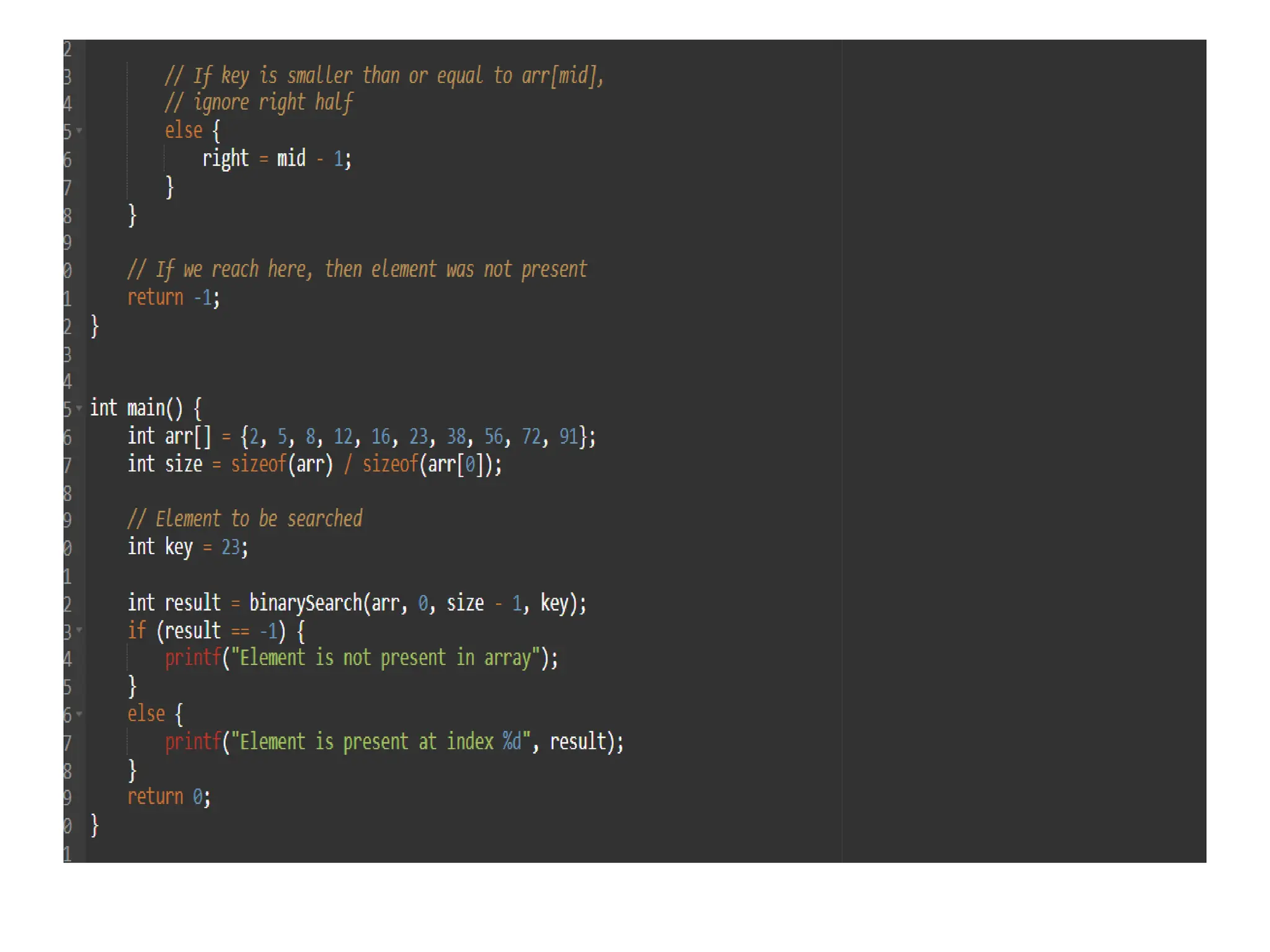
![• int main() { • This defines the main function, which is the entry point of the program. • int arr[] = {2, 5, 8, 12, 16, 23, 38, 56, 72, 91}; • An array of integers is defined. This is the sorted array where the binary search will be performed. • int size = sizeof(arr) / sizeof(arr[0]); • This calculates the size of the array by dividing the total size of the array by the size of a single element. • int key = 23; • This initializes the key variable with the value to be searched in the array. • int result = binarySearch(arr, 0, size - 1, key); • This calls the binarySearch function, passing the array, the left index (0), the right index (size - 1), and the key. The result (the index of the found element or -1) is stored in the variable result.](https://image.slidesharecdn.com/unit2daa-250905053837-430b107f/75/Design-and-analysis-of-algorithm-devide-and-conquer-63-2048.jpg)