Tree Data Structures with Types, Properties, Traversals, Advanced Variants, and Applications in Computer Science

Dr.M.Usha ASSOCIATE PROFESSOR, Department of CSE Velammal engineering College Velammal Engineering College (An Autonomous Institution, Affiliated to Anna University, Chennai) (Accredited by NAAC & NBA) NON LINEAR DATA STRUCTURES - BST

08/18/2025 VELAMMAL ENGINEERING COLLEGE, Dept. of CSE 2 CONTENTS  1) Introduction to Trees.  2) Basic terminologies  3) Binary tree  4) Binary tree types  5) Binary tree representation  6) Binary search tree  7) Creation of a binary tree  8) Operations on binary search tree Trees

08/18/2025 VELAMMAL ENGINEERING COLLEGE, Dept. of CSE 3 Nonlinear Data Structures  The data structure where data items are not organized sequentially is called non linear data structure.  A data item in a nonlinear data structure could be attached to several other data elements to reflect a special relationship among them and all the data items cannot be traversed in a single run.  Data structures like trees and graphs are some examples of widely used nonlinear data structures.

08/18/2025 VELAMMAL ENGINEERING COLLEGE, Dept. of CSE 4  A tree is a nonlinear hierarchical data structure that consists of nodes connected by edges .  It stores the information naturally in the form of hierarchical style.  In this, the data elements can be attached to more than one element exhibiting the hierarchical relationship which involves the relationship between the child, parent, and grandparent.  A tree can be empty with no nodes or a tree is a structure consisting of one node called the root and zero or one or more subtrees.  In a general tree, A node can have any number of children nodes but it can have only a single parent. TREE

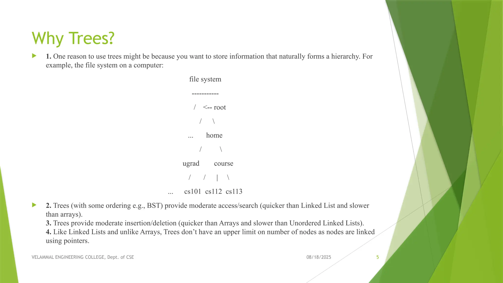
08/18/2025 VELAMMAL ENGINEERING COLLEGE, Dept. of CSE 5 Why Trees?  1. One reason to use trees might be because you want to store information that naturally forms a hierarchy. For example, the file system on a computer: file system ----------- / <-- root / ... home / ugrad course / / | ... cs101 cs112 cs113  2. Trees (with some ordering e.g., BST) provide moderate access/search (quicker than Linked List and slower than arrays). 3. Trees provide moderate insertion/deletion (quicker than Arrays and slower than Unordered Linked Lists). 4. Like Linked Lists and unlike Arrays, Trees don’t have an upper limit on number of nodes as nodes are linked using pointers.

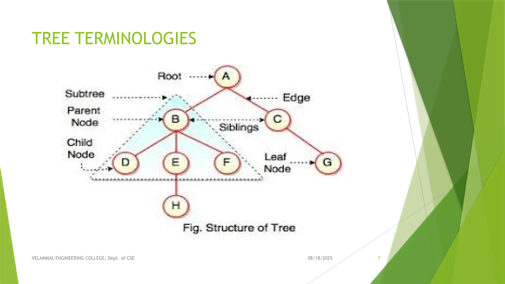
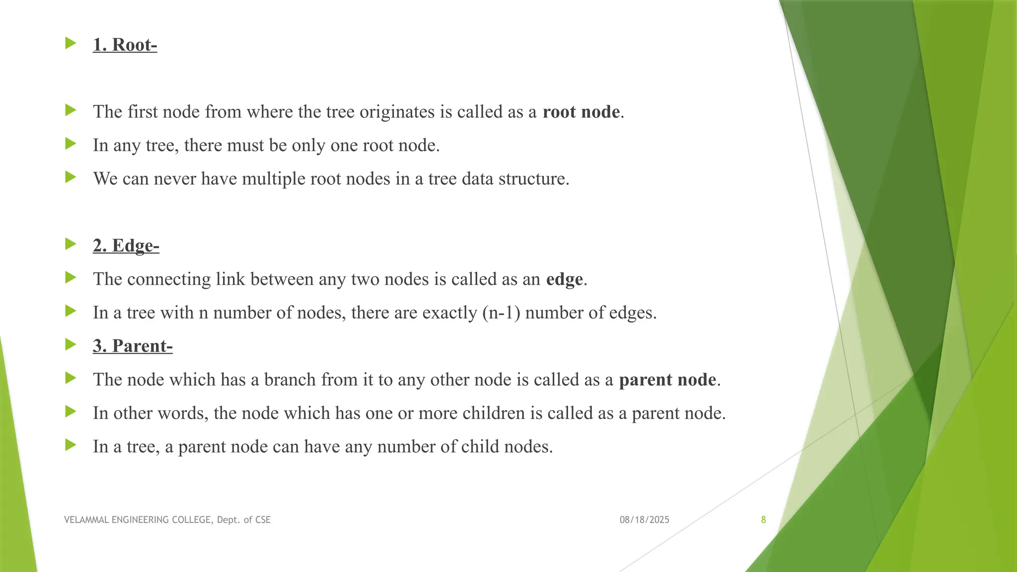
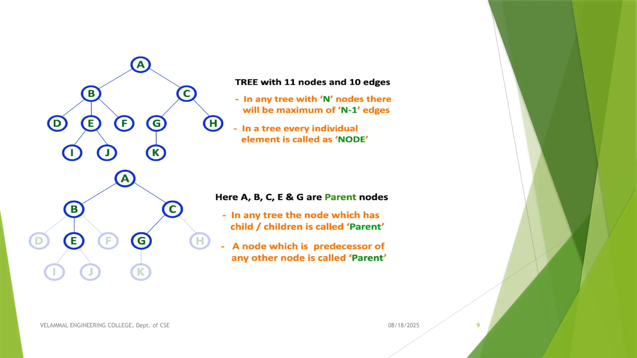
08/18/2025 VELAMMAL ENGINEERING COLLEGE, Dept. of CSE 6 TREE TERMINOLOGY

08/18/2025 VELAMMAL ENGINEERING COLLEGE, Dept. of CSE 7 TREE TERMINOLOGIES

08/18/2025 VELAMMAL ENGINEERING COLLEGE, Dept. of CSE 8  1. Root-  The first node from where the tree originates is called as a root node.  In any tree, there must be only one root node.  We can never have multiple root nodes in a tree data structure.  2. Edge-  The connecting link between any two nodes is called as an edge.  In a tree with n number of nodes, there are exactly (n-1) number of edges.  3. Parent-  The node which has a branch from it to any other node is called as a parent node.  In other words, the node which has one or more children is called as a parent node.  In a tree, a parent node can have any number of child nodes.

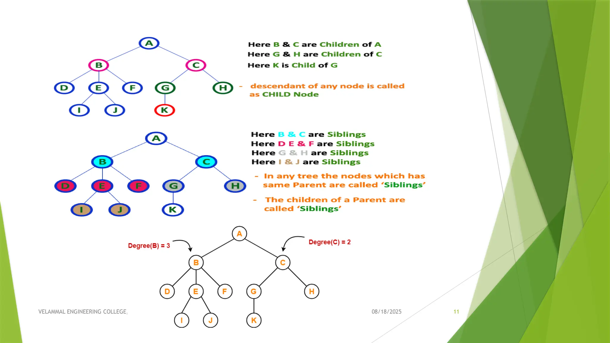
08/18/2025 VELAMMAL ENGINEERING COLLEGE, Dept. of CSE 9

08/18/2025 VELAMMAL ENGINEERING COLLEGE, Dept. of CSE 10  4. Child-  The node which is a descendant of some node is called as a child node.  All the nodes except root node are child nodes.  5. Siblings-  Nodes which belong to the same parent are called as siblings.  In other words, nodes with the same parent are sibling nodes.  6. Degree-  Degree of a node is the total number of children of that node.  Degree of a tree is the highest degree of a node among all the nodes in the tree.

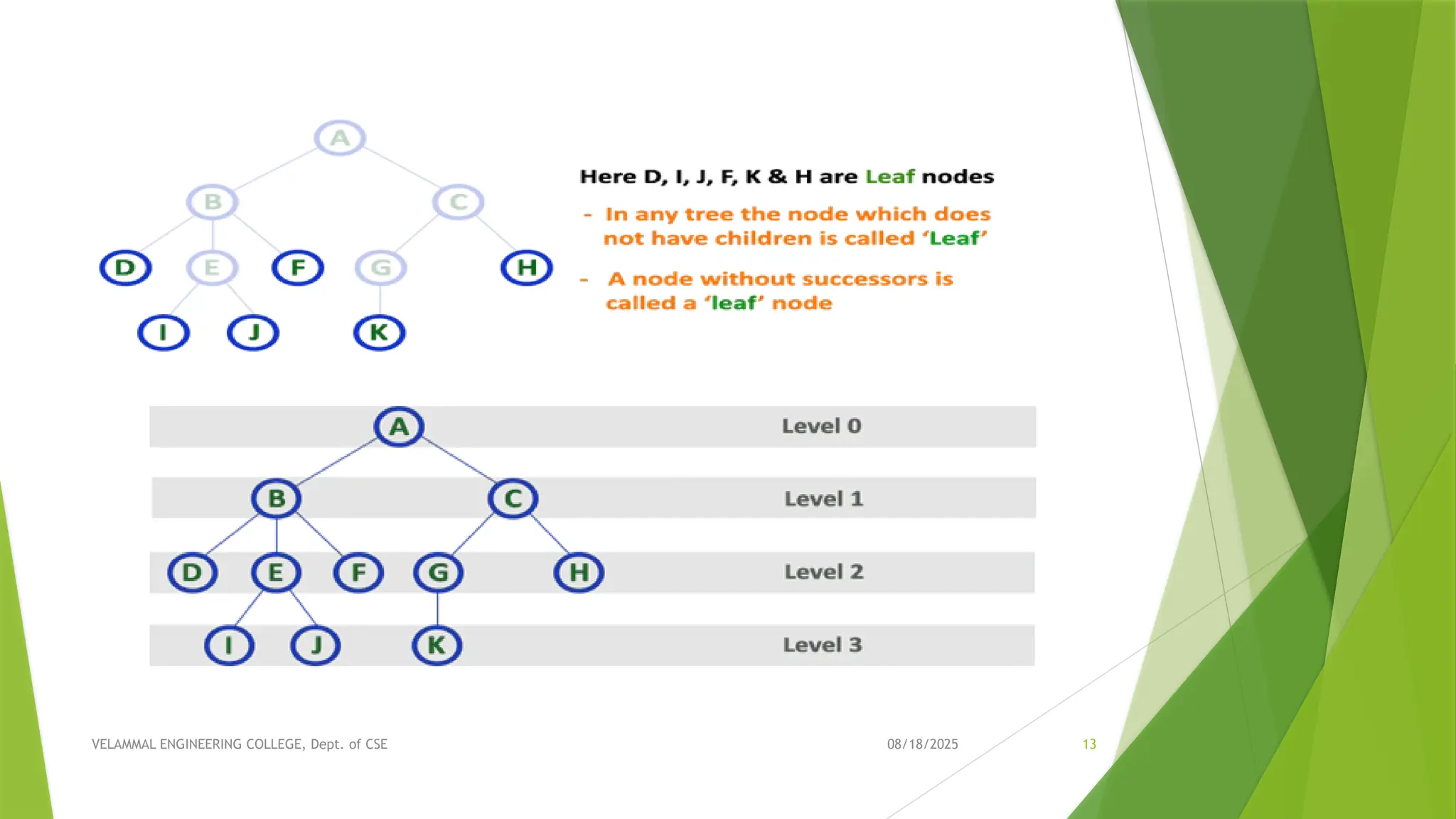
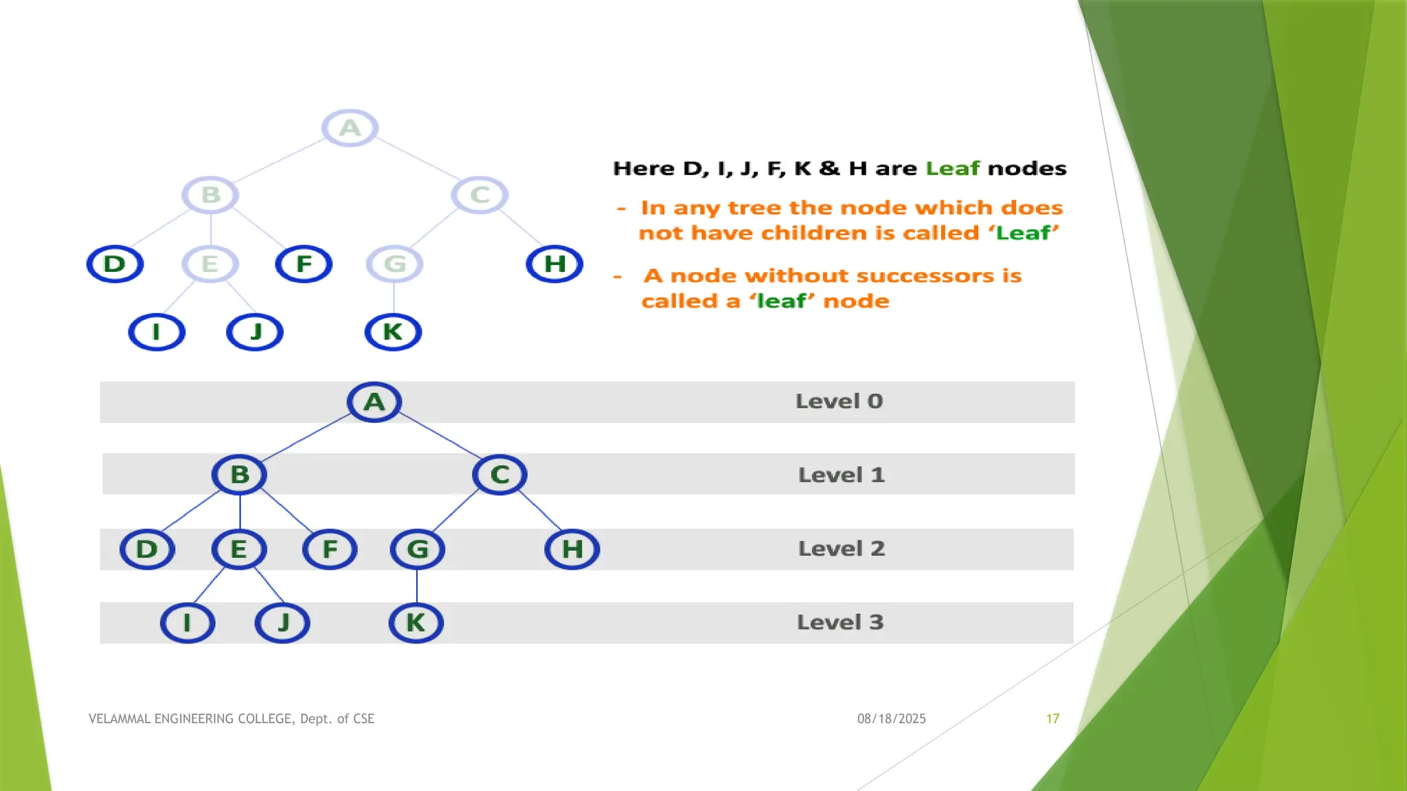
08/18/2025 VELAMMAL ENGINEERING COLLEGE, Dept. of CSE 12  7. Internal Node-  The node which has at least one child is called as an internal node.  Internal nodes are also called as non-terminal nodes.  Every non-leaf node is an internal node.  8. Leaf Node-  The node which does not have any child is called as a leaf node.  Leaf nodes are also called as external nodes or terminal nodes.  9. Level-  In a tree, each step from top to bottom is called as level of a tree.  The level count starts with 0 and increments by 1 at each level or step.

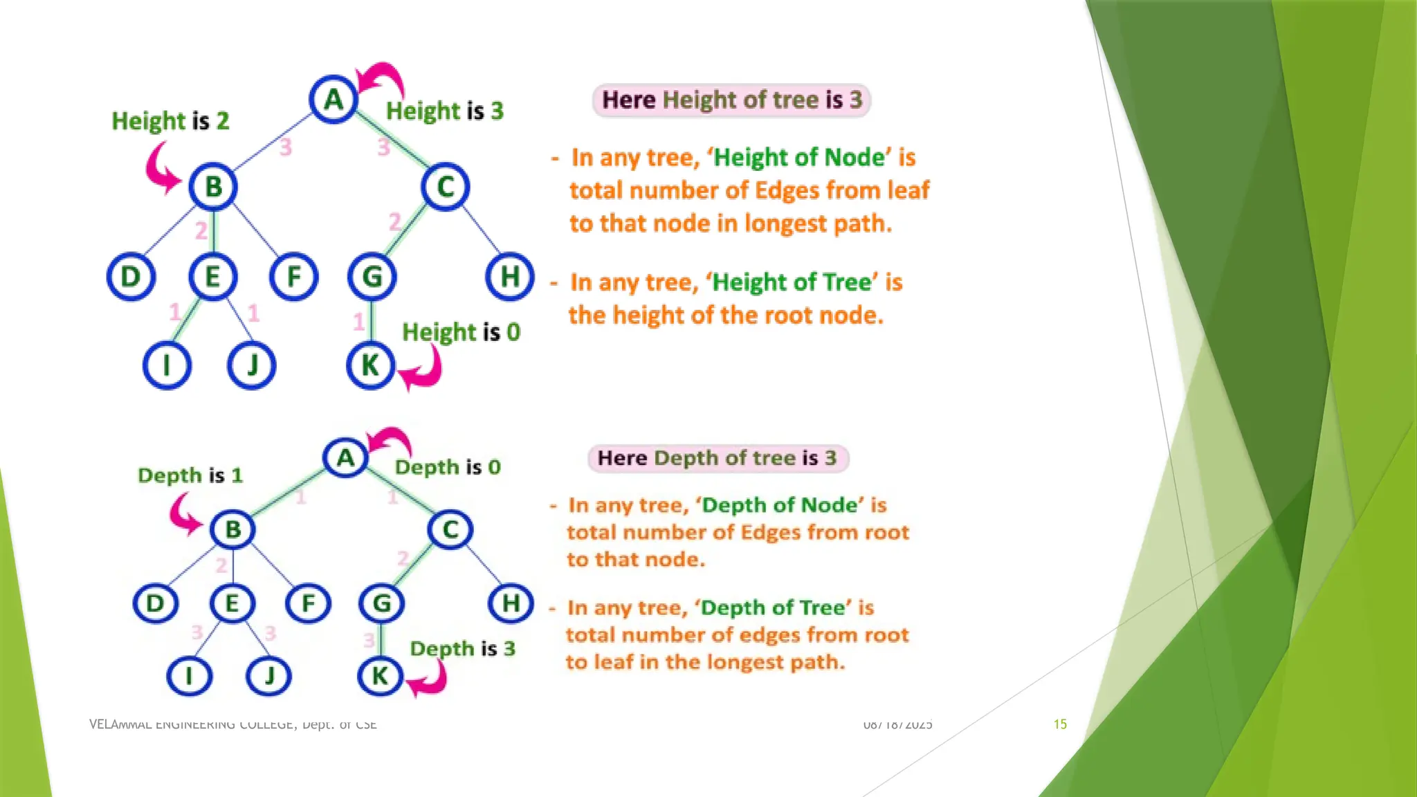
08/18/2025 VELAMMAL ENGINEERING COLLEGE, Dept. of CSE 14  10. Height-  Total number of edges that lies on the longest path from any leaf node to a particular node is called as height of that node.  Height of a tree is the height of root node.  Height of all leaf nodes = 0  11. Depth-  Total number of edges from root node to a particular node is called as depth of that node.  Depth of a tree is the total number of edges from root node to a leaf node in the longest path.  Depth of the root node = 0  The terms “level” and “depth” are used interchangeably.

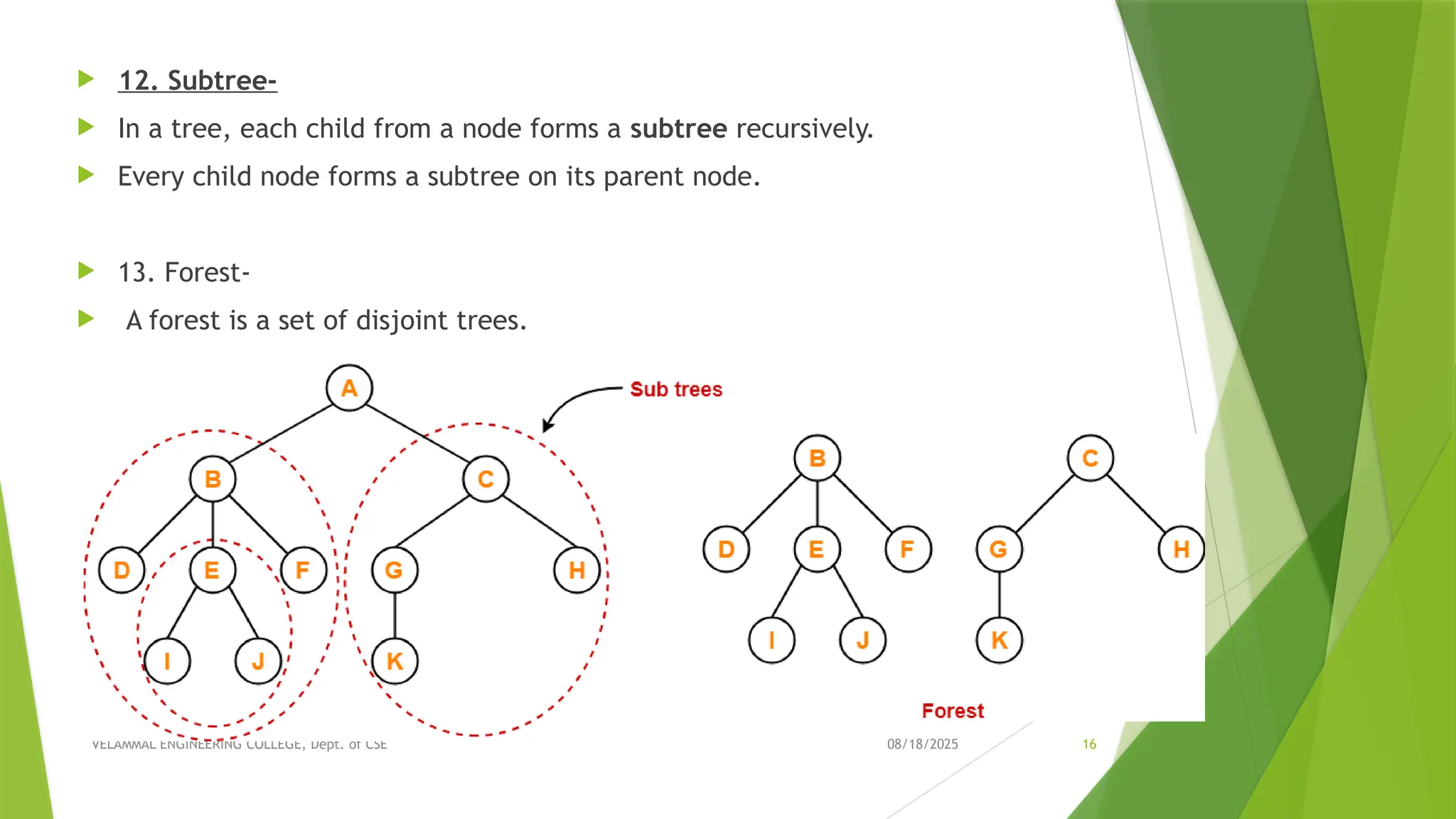
08/18/2025 VELAMMAL ENGINEERING COLLEGE, Dept. of CSE 16  12. Subtree-  In a tree, each child from a node forms a subtree recursively.  Every child node forms a subtree on its parent node.  13. Forest-  A forest is a set of disjoint trees.

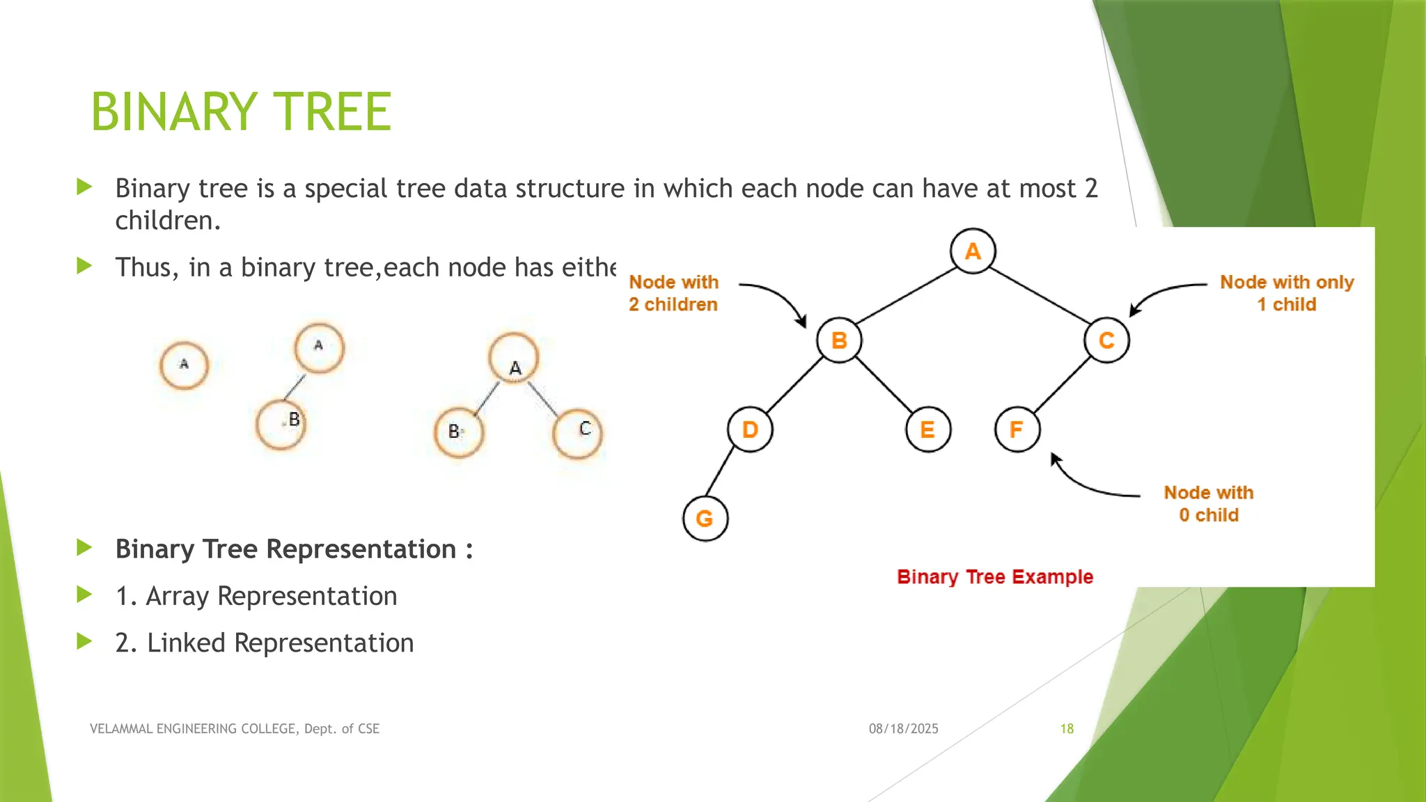
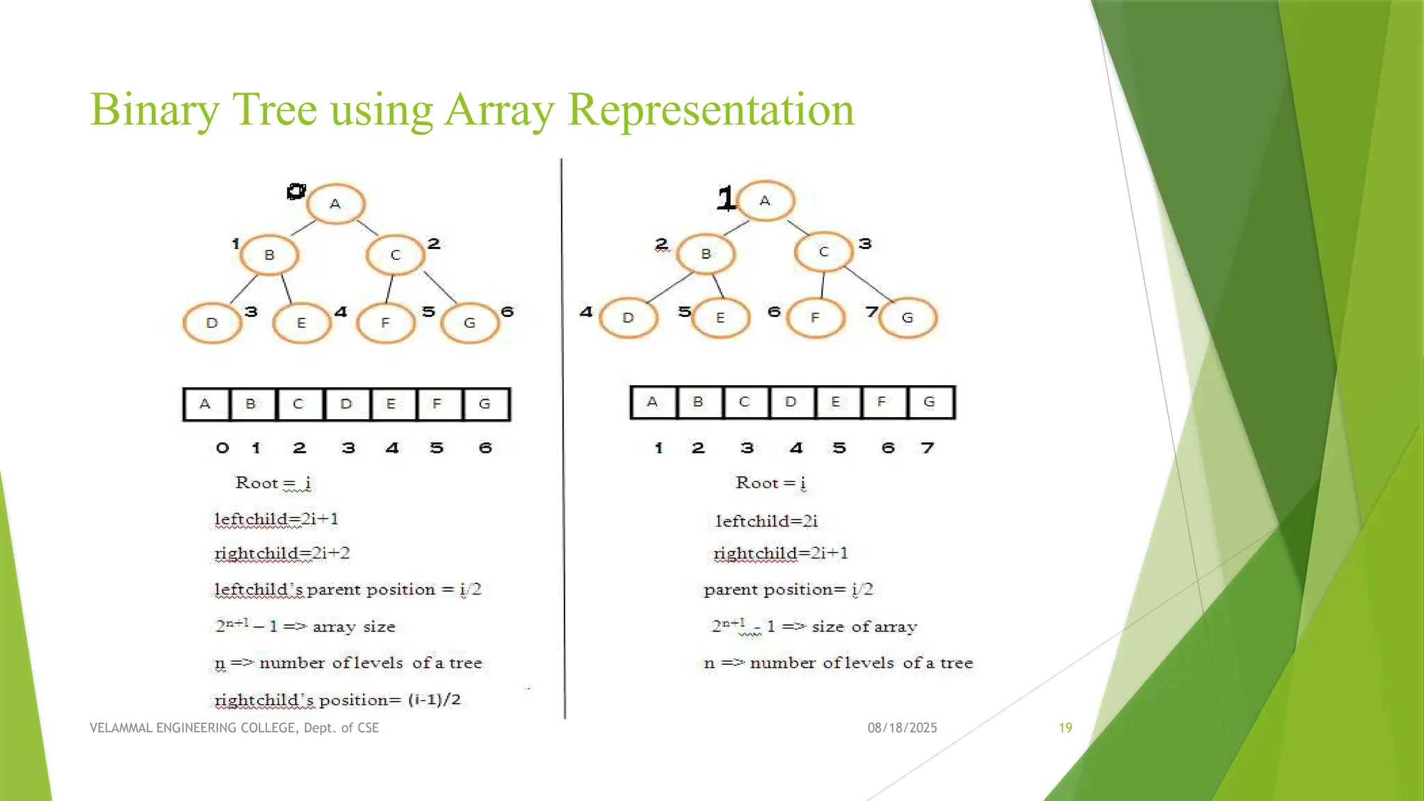
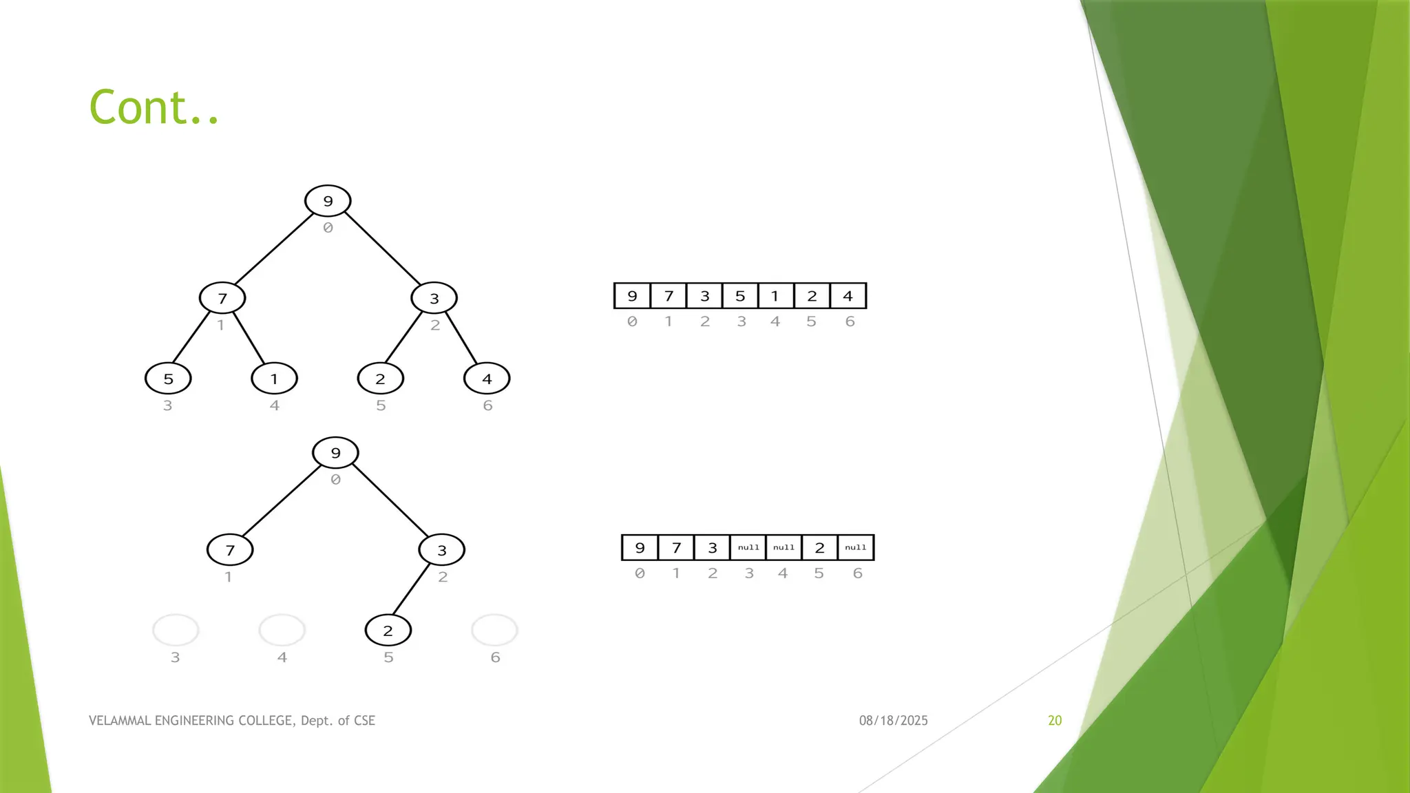
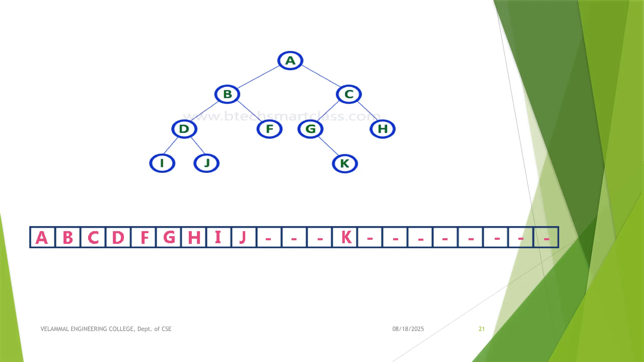
08/18/2025 VELAMMAL ENGINEERING COLLEGE, Dept. of CSE 18 BINARY TREE  Binary tree is a special tree data structure in which each node can have at most 2 children.  Thus, in a binary tree,each node has either 0 child or 1 child or 2 children.  Binary Tree Representation :  1. Array Representation  2. Linked Representation

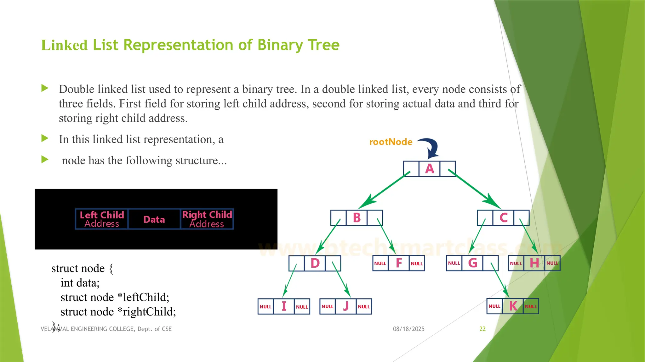
08/18/2025 VELAMMAL ENGINEERING COLLEGE, Dept. of CSE 19 Binary Tree using Array Representation

08/18/2025 VELAMMAL ENGINEERING COLLEGE, Dept. of CSE 20 Cont..

08/18/2025 VELAMMAL ENGINEERING COLLEGE, Dept. of CSE 22 Linked List Representation of Binary Tree  Double linked list used to represent a binary tree. In a double linked list, every node consists of three fields. First field for storing left child address, second for storing actual data and third for storing right child address.  In this linked list representation, a  node has the following structure... struct node { int data; struct node *leftChild; struct node *rightChild; };

08/18/2025 VELAMMAL ENGINEERING COLLEGE, Dept. of CSE 23 Types of Binary Trees-  FULL BINARY TREE  PERFECT BINARY TREE  COMPLETE BINARY TREE  SKEWED BINARY TREE

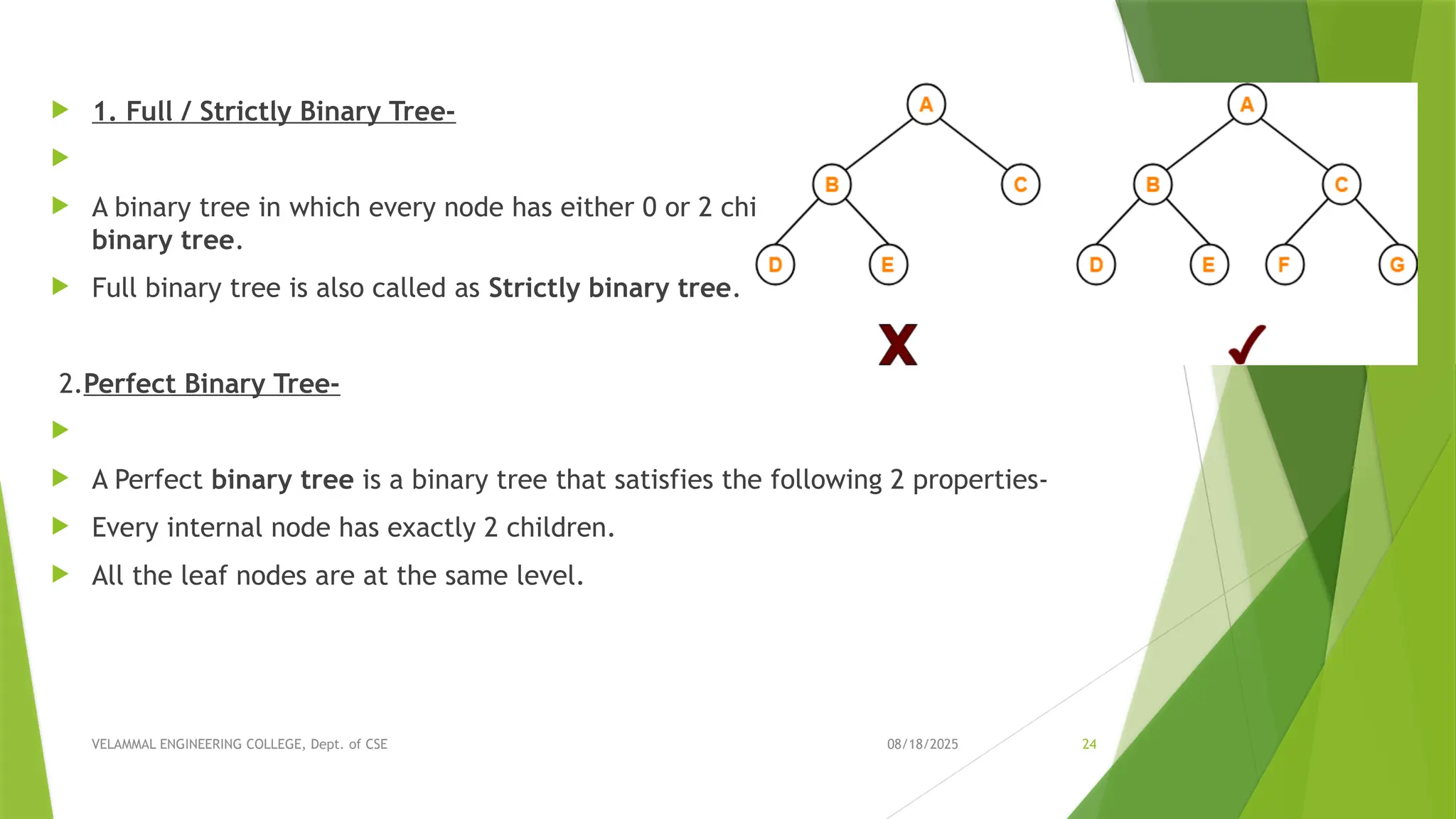
08/18/2025 VELAMMAL ENGINEERING COLLEGE, Dept. of CSE 24  1. Full / Strictly Binary Tree-   A binary tree in which every node has either 0 or 2 children is called as a Full binary tree.  Full binary tree is also called as Strictly binary tree. 2.Perfect Binary Tree-   A Perfect binary tree is a binary tree that satisfies the following 2 properties-  Every internal node has exactly 2 children.  All the leaf nodes are at the same level.

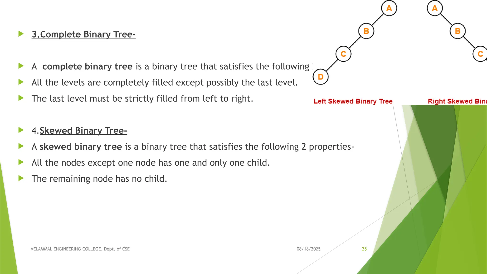
08/18/2025 VELAMMAL ENGINEERING COLLEGE, Dept. of CSE 25  3.Complete Binary Tree-  A complete binary tree is a binary tree that satisfies the following 2 properties-  All the levels are completely filled except possibly the last level.  The last level must be strictly filled from left to right.  4.Skewed Binary Tree-  A skewed binary tree is a binary tree that satisfies the following 2 properties-  All the nodes except one node has one and only one child.  The remaining node has no child.

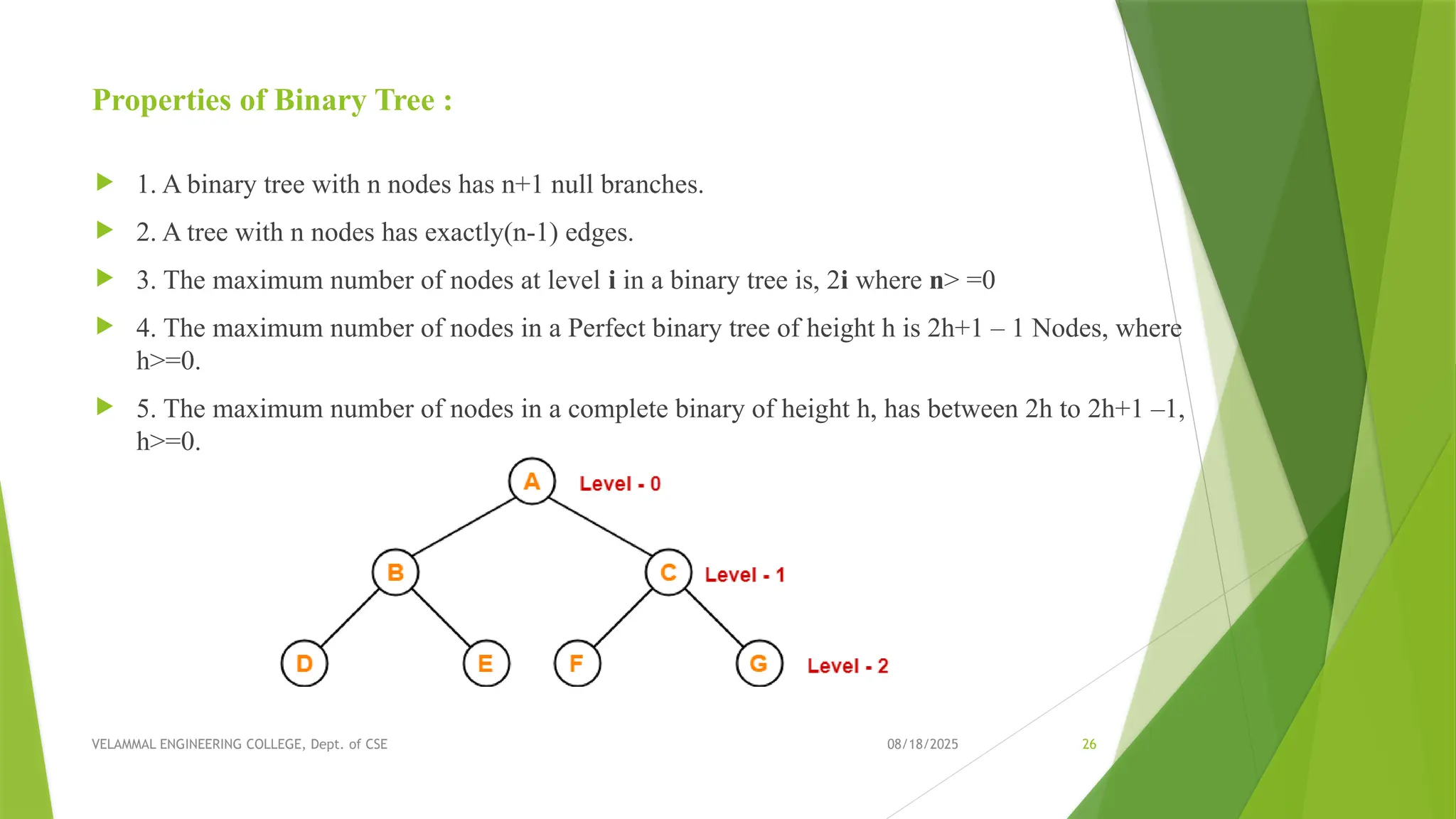
08/18/2025 VELAMMAL ENGINEERING COLLEGE, Dept. of CSE 26 Properties of Binary Tree :  1. A binary tree with n nodes has n+1 null branches.  2. A tree with n nodes has exactly(n-1) edges.  3. The maximum number of nodes at level i in a binary tree is, 2i where n> =0  4. The maximum number of nodes in a Perfect binary tree of height h is 2h+1 – 1 Nodes, where h>=0.  5. The maximum number of nodes in a complete binary of height h, has between 2h to 2h+1 –1, h>=0.

08/18/2025 VELAMMAL ENGINEERING COLLEGE, Dept. of CSE 27 Binary Tree Traversals  Displaying (or) visiting order of nodes in a binary tree is called as Binary Tree Traversal.  There are three types of binary tree traversals.  In - Order Traversal  Pre - Order Traversal  Post - Order Traversal

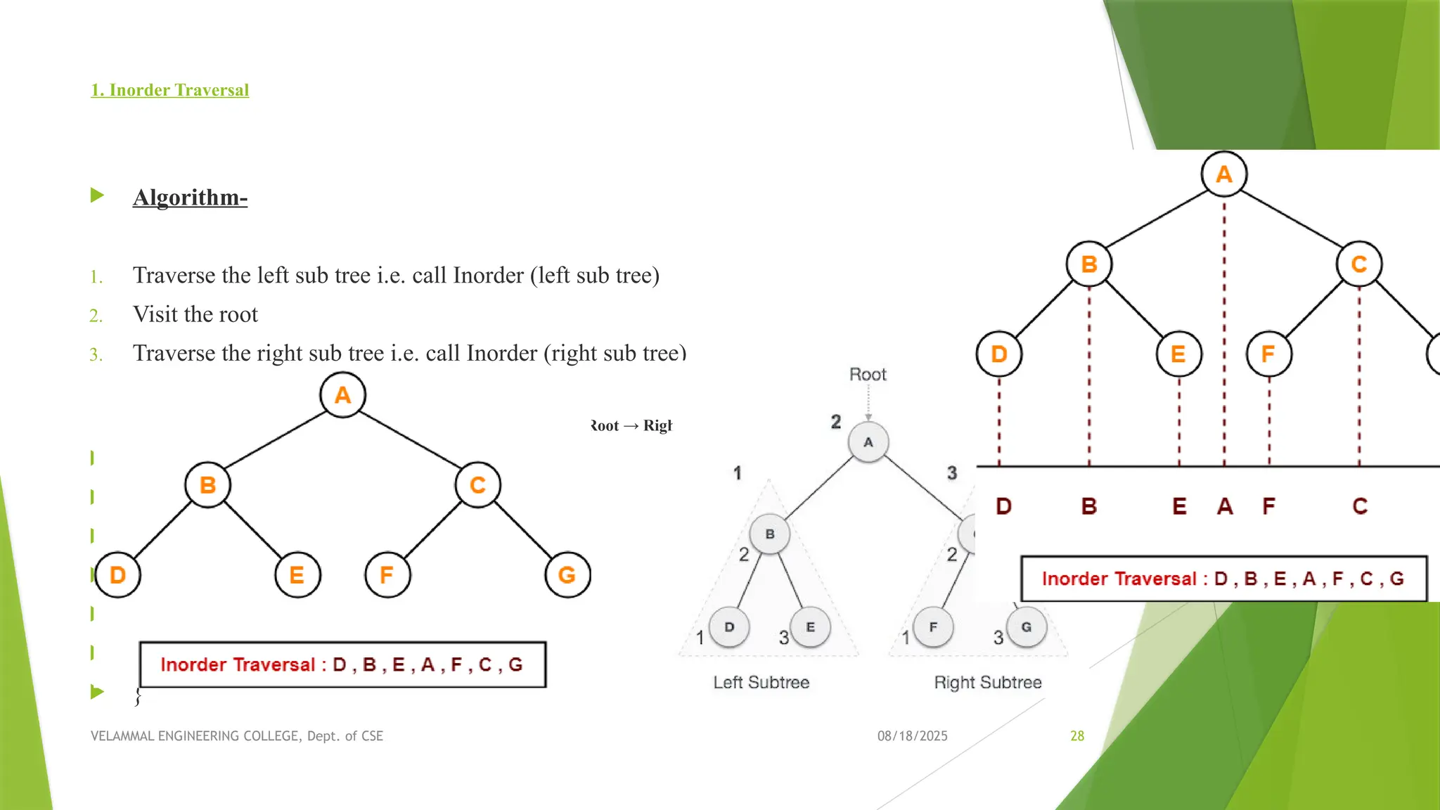
08/18/2025 VELAMMAL ENGINEERING COLLEGE, Dept. of CSE 28 1. Inorder Traversal  Algorithm- 1. Traverse the left sub tree i.e. call Inorder (left sub tree) 2. Visit the root 3. Traverse the right sub tree i.e. call Inorder (right sub tree)  Left → Root → Right  void inorder_traversal(struct node* root) {  if(root != NULL) {  inorder_traversal(root->leftChild);  printf("%d ",root->data);  inorder_traversal(root->rightChild);  }  }

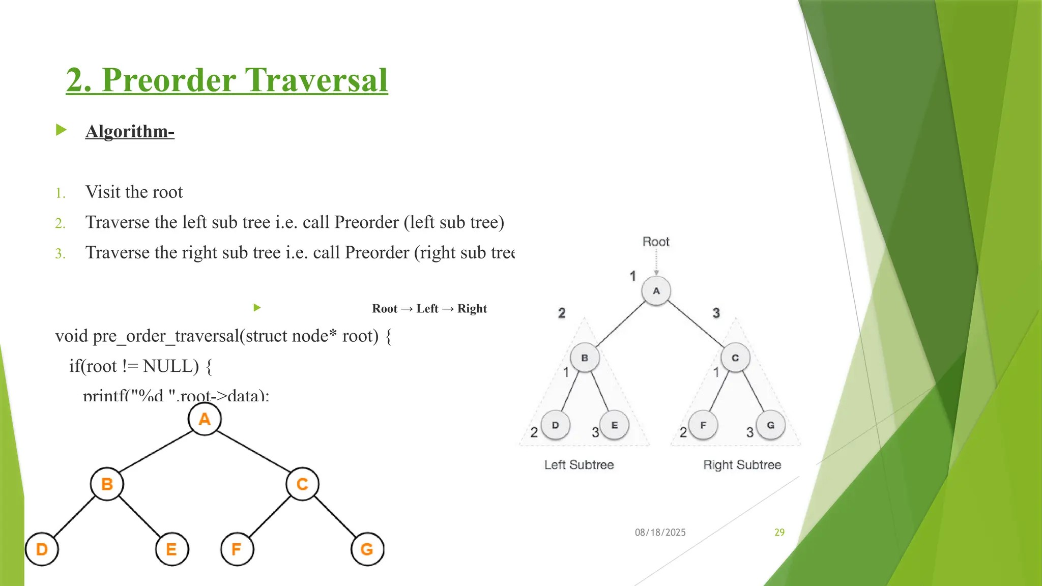
08/18/2025 VELAMMAL ENGINEERING COLLEGE, Dept. of CSE 29 2. Preorder Traversal  Algorithm- 1. Visit the root 2. Traverse the left sub tree i.e. call Preorder (left sub tree) 3. Traverse the right sub tree i.e. call Preorder (right sub tree)  Root → Left → Right void pre_order_traversal(struct node* root) { if(root != NULL) { printf("%d ",root->data); pre_order_traversal(root->leftChild); pre_order_traversal(root->rightChild); } }

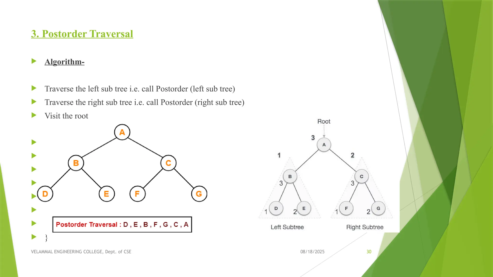
08/18/2025 VELAMMAL ENGINEERING COLLEGE, Dept. of CSE 30 3. Postorder Traversal  Algorithm-  Traverse the left sub tree i.e. call Postorder (left sub tree)  Traverse the right sub tree i.e. call Postorder (right sub tree)  Visit the root  Left → Right → Root  void post_order_traversal(struct node* root) {  if(root != NULL) {  post_order_traversal(root->leftChild);  post_order_traversal(root->rightChild);  printf("%d ", root->data);  }  }

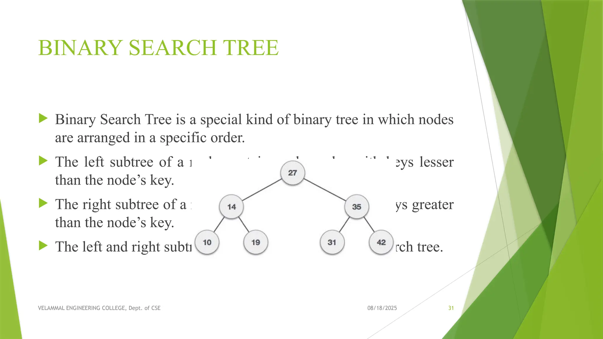
08/18/2025 VELAMMAL ENGINEERING COLLEGE, Dept. of CSE 31 BINARY SEARCH TREE  Binary Search Tree is a special kind of binary tree in which nodes are arranged in a specific order.  The left subtree of a node contains only nodes with keys lesser than the node’s key.  The right subtree of a node contains only nodes with keys greater than the node’s key.  The left and right subtree each must also be a binary search tree.

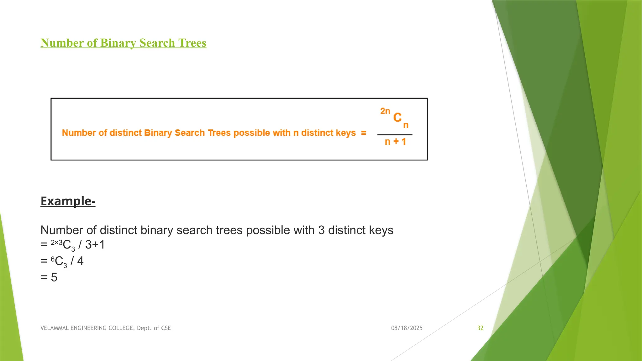
08/18/2025 VELAMMAL ENGINEERING COLLEGE, Dept. of CSE 32 Number of Binary Search Trees Example- Number of distinct binary search trees possible with 3 distinct keys = 2×3 C3 / 3+1 = 6 C3 / 4 = 5

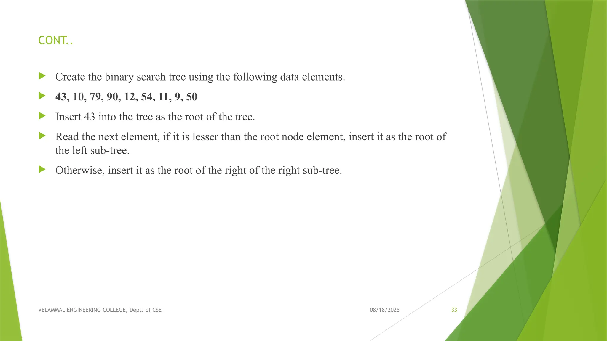
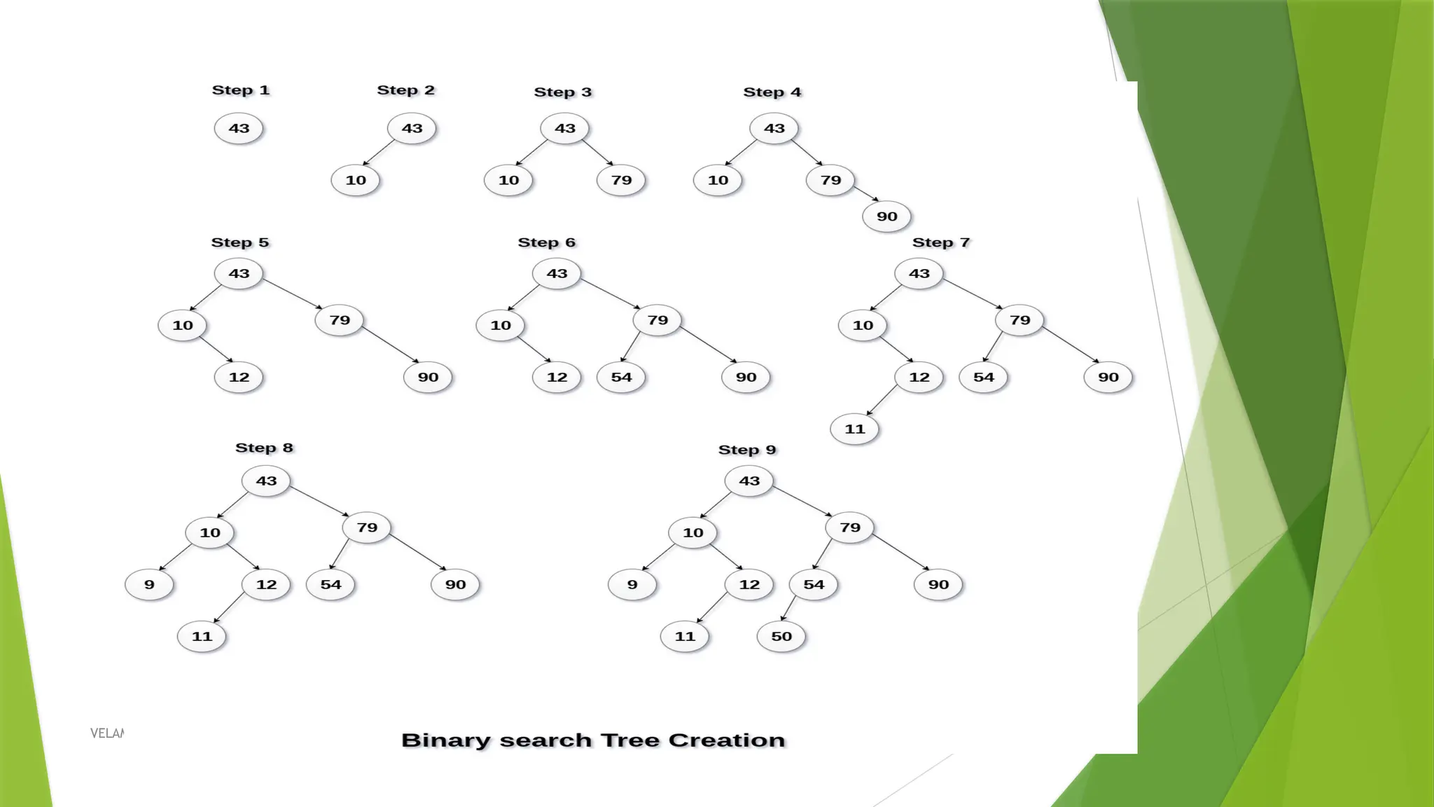
08/18/2025 VELAMMAL ENGINEERING COLLEGE, Dept. of CSE 33 CONT..  Create the binary search tree using the following data elements.  43, 10, 79, 90, 12, 54, 11, 9, 50  Insert 43 into the tree as the root of the tree.  Read the next element, if it is lesser than the root node element, insert it as the root of the left sub-tree.  Otherwise, insert it as the root of the right of the right sub-tree.

08/18/2025 VELAMMAL ENGINEERING COLLEGE, Dept. of CSE 36 Operations on BST  Insert an element – Delete an element – Search for an element – Find the minimum/maximum element – Find the successor/predecessor of a node.  Basic operations of a tree  Search − Searches an element in a tree.  FindMin – Find Minimum element in a tree  FindMax – Find Maximum element in a tree  Insert − Inserts an element in a tree.  Delete − deletes an element in a tree.  Pre-order Traversal − Traverses a tree in a pre-order manner.  In-order Traversal − Traverses a tree in an in-order manner.  Post-order Traversal − Traverses a tree in a post-order manner.

08/18/2025 VELAMMAL ENGINEERING COLLEGE, Dept. of CSE 37 1. Search Operation  Search Operation is performed to search a particular element in the Binary Search Tree.  Rules-  For searching a given key in the BST,  Compare the key with the value of root node.  If the key is present at the root node, then return the root node.  If the key is greater than the root node value, then recur for the root node’s right subtree.  If the key is smaller than the root node value, then recur for the root node’s left subtree.

08/18/2025 VELAMMAL ENGINEERING COLLEGE, Dept. of CSE 38 Algorithm: Search (ROOT, ITEM) •Step 1: IF ROOT -> DATA = ITEM OR ROOT = NULL Return ROOT ELSE IF ITEM < ROOT -> DATA Return search(ROOT -> LEFT, ITEM) ELSE Return search(ROOT -> RIGHT,ITEM) [END OF IF] [END OF IF] •Step 2: END

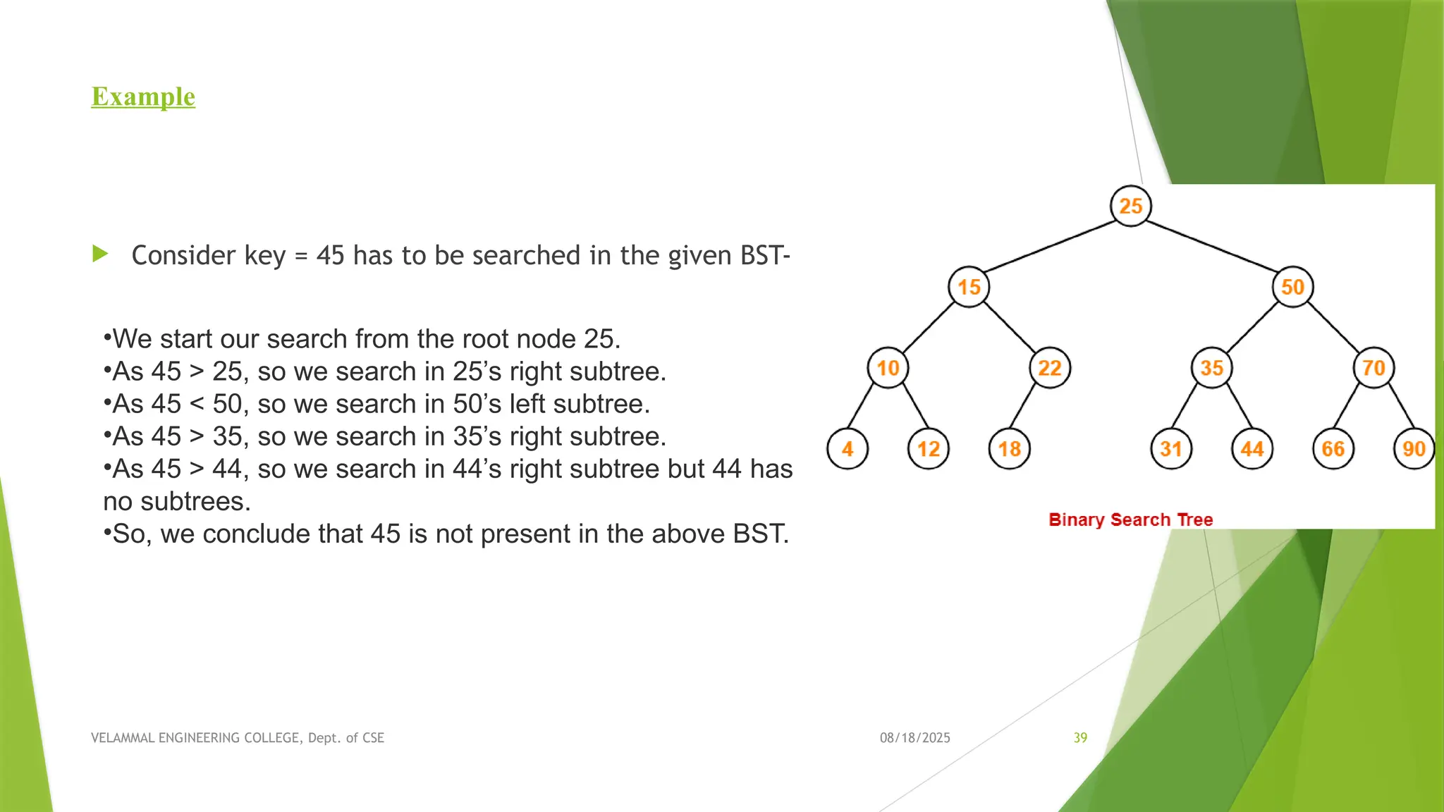
08/18/2025 VELAMMAL ENGINEERING COLLEGE, Dept. of CSE 39 Example  Consider key = 45 has to be searched in the given BST- •We start our search from the root node 25. •As 45 > 25, so we search in 25’s right subtree. •As 45 < 50, so we search in 50’s left subtree. •As 45 > 35, so we search in 35’s right subtree. •As 45 > 44, so we search in 44’s right subtree but 44 has no subtrees. •So, we conclude that 45 is not present in the above BST.

08/18/2025 VELAMMAL ENGINEERING COLLEGE, Dept. of CSE 40 2. Insertion Operation  Rules-  Insert function is used to add a new element in a binary search tree at appropriate location. Insert function is to be designed in such a way that, it must node violate the property of binary search tree at each value.  Allocate the memory for tree.  Set the data part to the value and set the left and right pointer of tree, point to NULL.  If the item to be inserted, will be the first element of the tree, then the left and right of this node will point to NULL.  Else, check if the item is less than the root element of the tree, if this is true, then recursively perform this operation with the left of the root.  If this is false, then perform this operation recursively with the right sub-tree of the root.

08/18/2025 VELAMMAL ENGINEERING COLLEGE, Dept. of CSE 41 Insert (TREE, ITEM) •Step 1: IF ROOT = NULL Allocate memory for TREE SET ROOT -> DATA = ITEM SET ROOT -> LEFT = ROOT -> RIGHT = NULL ELSE IF ITEM < ROOT -> DATA Insert(ROOT -> LEFT, ITEM) ELSE Insert(ROOT -> RIGHT, ITEM) [END OF IF] [END OF IF] •Step 2: END

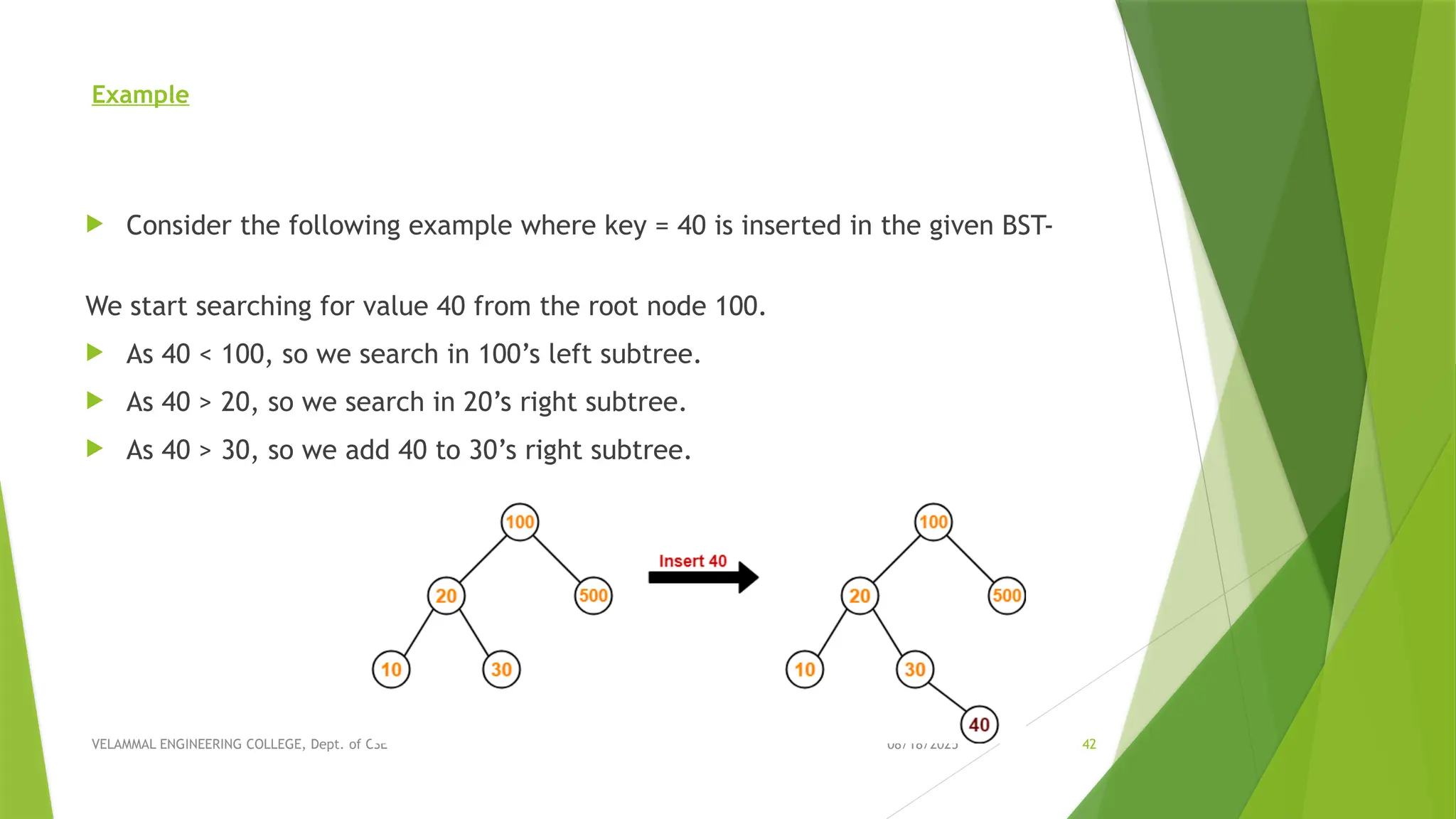
08/18/2025 VELAMMAL ENGINEERING COLLEGE, Dept. of CSE 42 Example  Consider the following example where key = 40 is inserted in the given BST- We start searching for value 40 from the root node 100.  As 40 < 100, so we search in 100’s left subtree.  As 40 > 20, so we search in 20’s right subtree.  As 40 > 30, so we add 40 to 30’s right subtree.

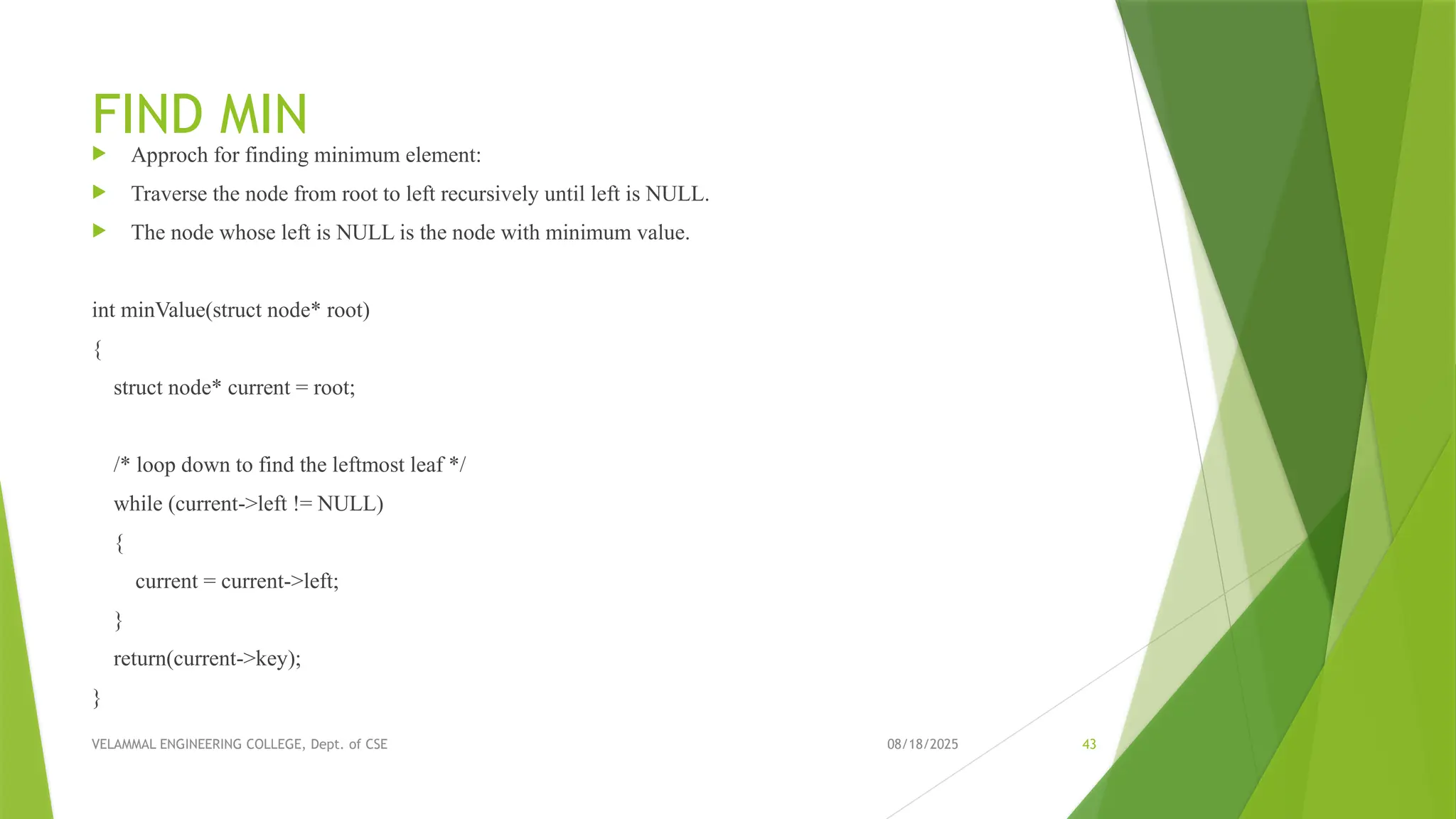
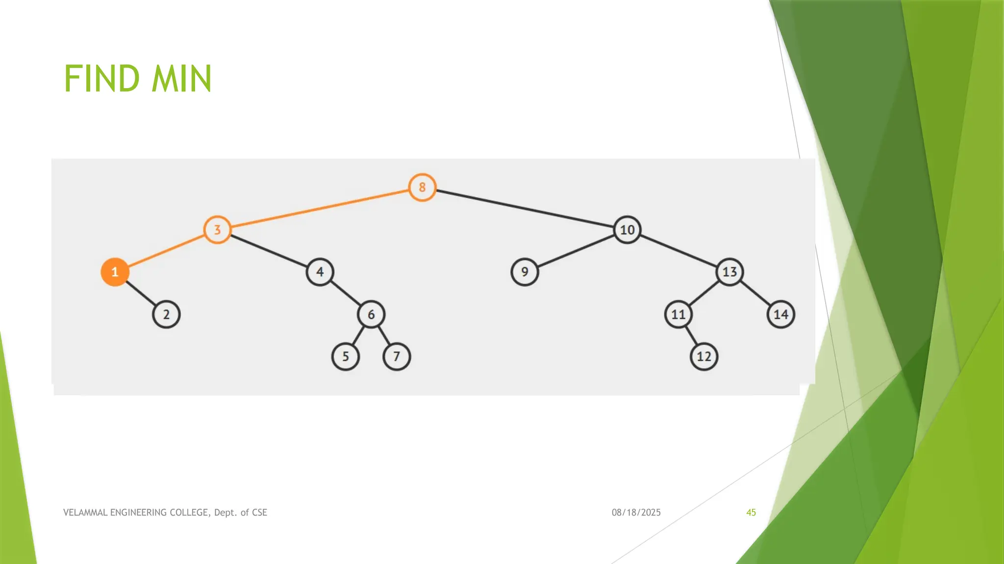
08/18/2025 VELAMMAL ENGINEERING COLLEGE, Dept. of CSE 43 FIND MIN  Approch for finding minimum element:  Traverse the node from root to left recursively until left is NULL.  The node whose left is NULL is the node with minimum value. int minValue(struct node* root) { struct node* current = root; /* loop down to find the leftmost leaf */ while (current->left != NULL) { current = current->left; } return(current->key); }

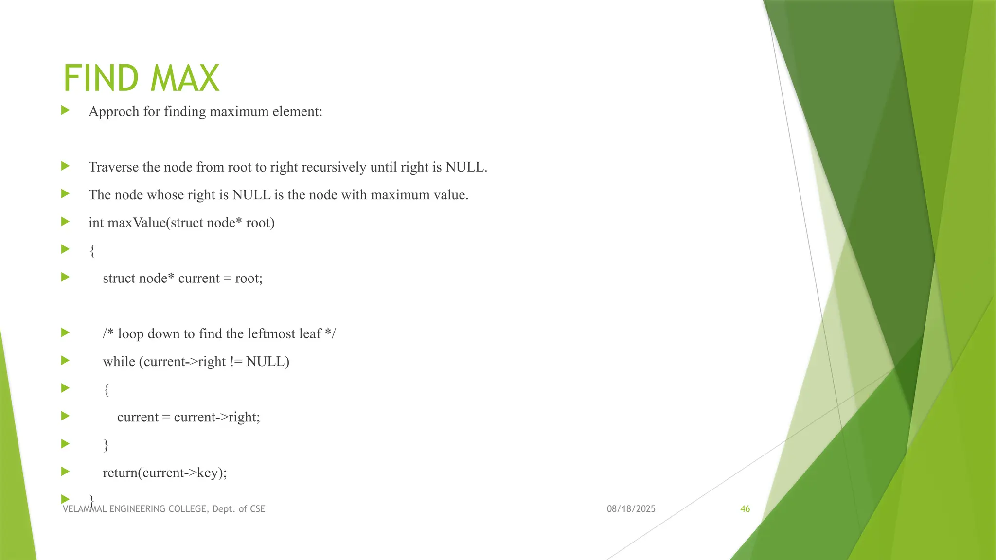
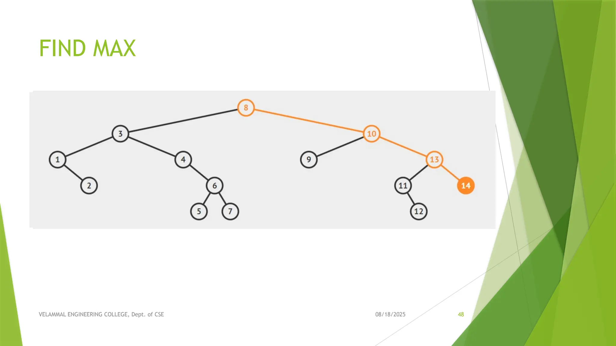
08/18/2025 VELAMMAL ENGINEERING COLLEGE, Dept. of CSE 44 find_min( struct btree *t ) { if( T == NULL ) return NULL; else if( T->left == NULL ) return( T ); else return( find_min ( T->left ) ); }

08/18/2025 VELAMMAL ENGINEERING COLLEGE, Dept. of CSE 45 FIND MIN

08/18/2025 VELAMMAL ENGINEERING COLLEGE, Dept. of CSE 46 FIND MAX  Approch for finding maximum element:  Traverse the node from root to right recursively until right is NULL.  The node whose right is NULL is the node with maximum value.  int maxValue(struct node* root)  {  struct node* current = root;  /* loop down to find the leftmost leaf */  while (current->right != NULL)  {  current = current->right;  }  return(current->key);  }

08/18/2025 VELAMMAL ENGINEERING COLLEGE, Dept. of CSE 47 find_min( struct btree *t ) { if( T == NULL ) return NULL; else if( T->right == NULL ) return( T ); else return( find_max ( T->right) ); }

08/18/2025 VELAMMAL ENGINEERING COLLEGE, Dept. of CSE 48 FIND MAX

08/18/2025 VELAMMAL ENGINEERING COLLEGE, Dept. of CSE 49 Time Complexity:  O(N) Worst case happens for left skewed trees in finding the minimum value. O(N) Worst case happens for right skewed trees in finding the maximum value.  O(1) Best case happens for left skewed trees in finding the maximum value. O(1) Best case happens for right skewed trees in finding the minimum value.

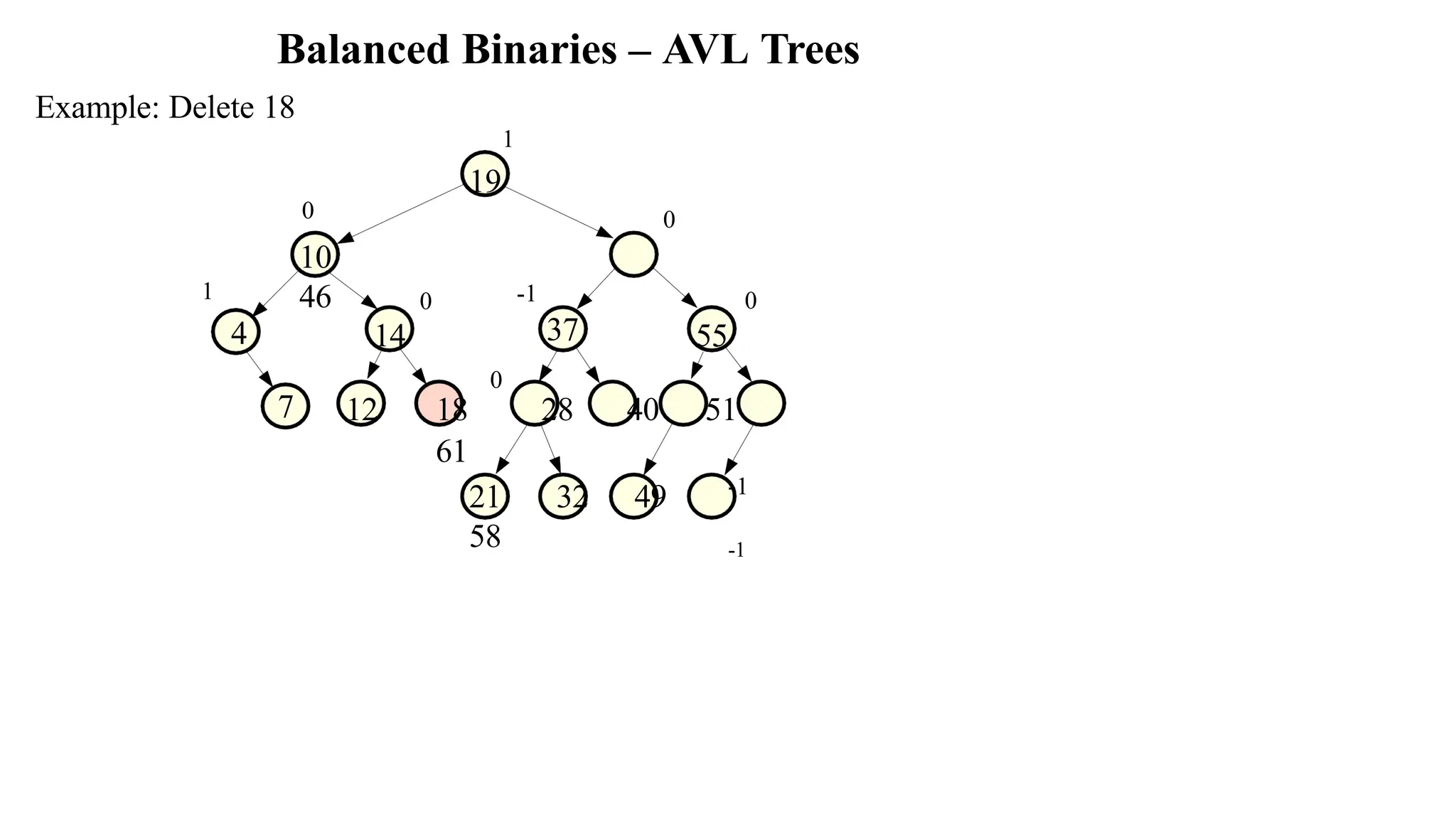
08/18/2025 VELAMMAL ENGINEERING COLLEGE, Dept. of CSE 50 3. Deletion Operation  Deletion Operation is performed to delete a particular element from the Binary Search Tree. • Case-01: Deletion Of A Node Having No Child (Leaf Node) • Case-02: Deletion Of A Node Having Only One Child • Case-02: Deletion Of A Node Having Two Children

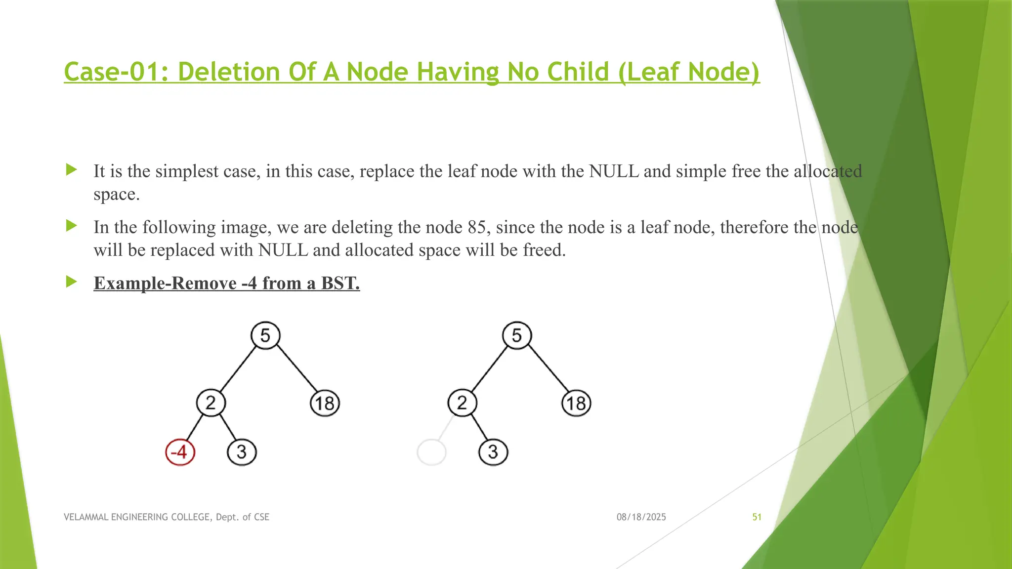
08/18/2025 VELAMMAL ENGINEERING COLLEGE, Dept. of CSE 51 Case-01: Deletion Of A Node Having No Child (Leaf Node)  It is the simplest case, in this case, replace the leaf node with the NULL and simple free the allocated space.  In the following image, we are deleting the node 85, since the node is a leaf node, therefore the node will be replaced with NULL and allocated space will be freed.  Example-Remove -4 from a BST.

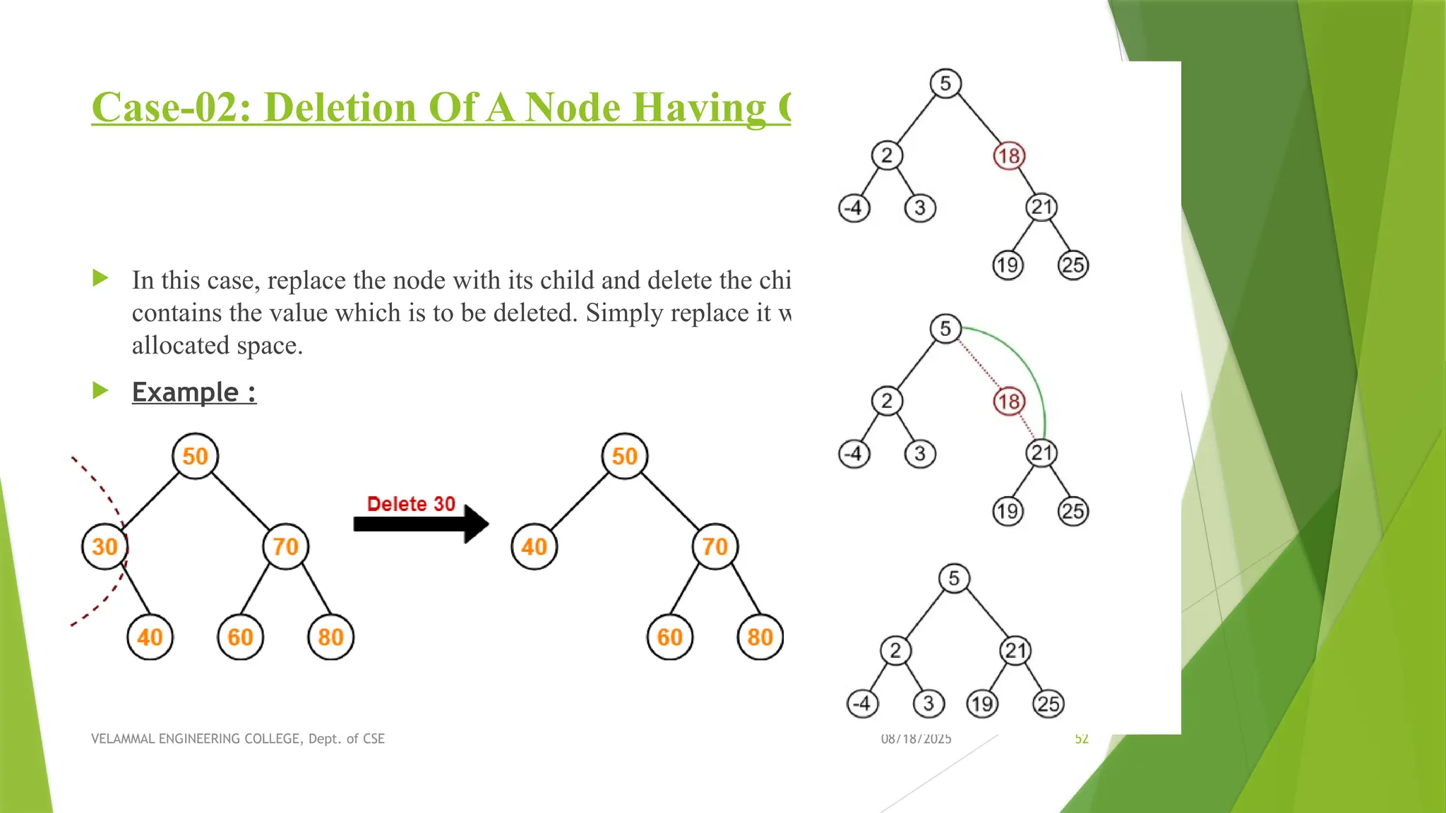
08/18/2025 VELAMMAL ENGINEERING COLLEGE, Dept. of CSE 52 Case-02: Deletion Of A Node Having Only One Child  In this case, replace the node with its child and delete the child node, which now contains the value which is to be deleted. Simply replace it with the NULL and free the allocated space.  Example :

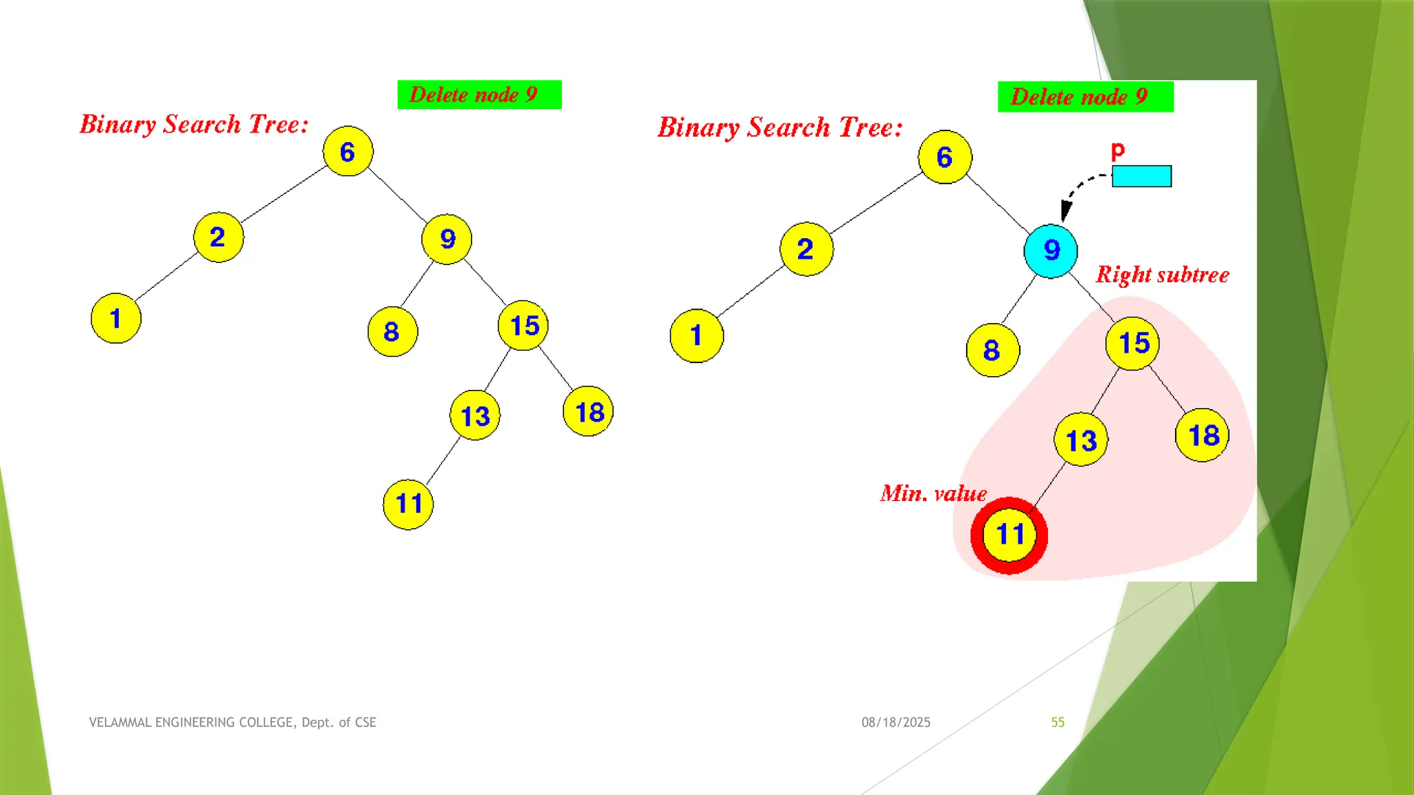
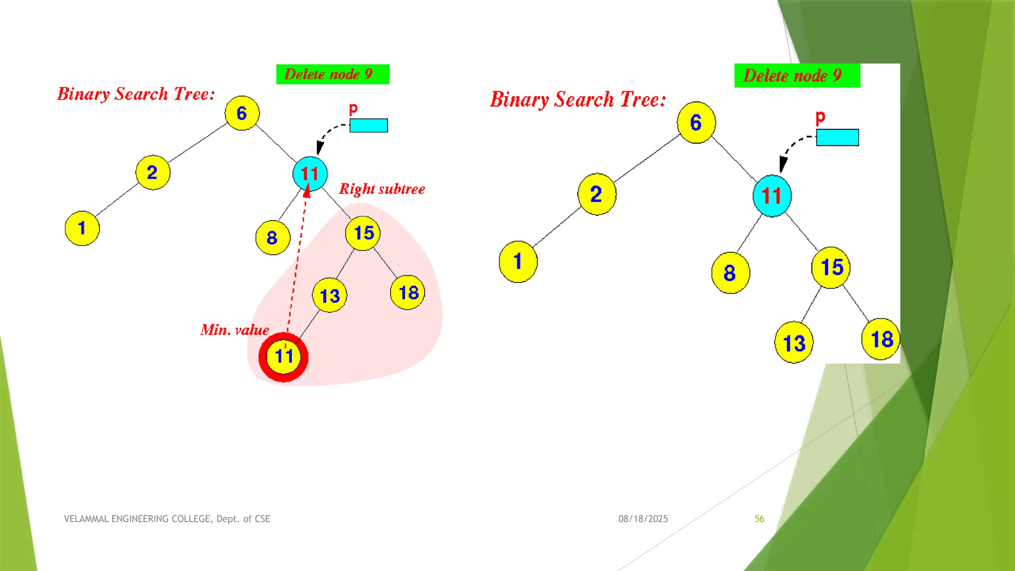
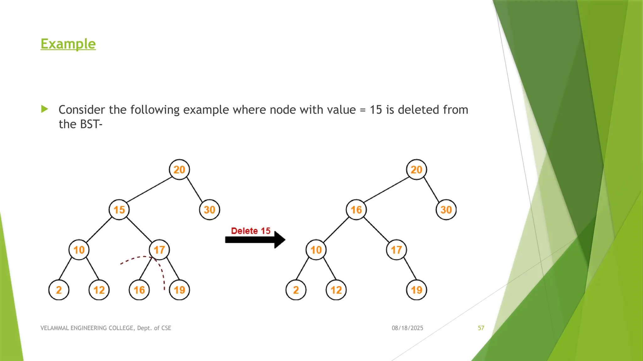
08/18/2025 VELAMMAL ENGINEERING COLLEGE, Dept. of CSE 53 Case-02: Deletion Of A Node Having Two Children  A node with two children may be deleted from the BST in the following two ways-  Method-01:  Visit to the right subtree of the deleting node.  Pluck the least value element called as inorder successor.  Replace the deleting element with its inorder successor.

08/18/2025 VELAMMAL ENGINEERING COLLEGE, Dept. of CSE 54  Algorithm  Delete (TREE, ITEM)  Step 1: IF TREE = NULL Write "item not found in the tree" ELSE IF ITEM < TREE -> DATA Delete(TREE->LEFT, ITEM) ELSE IF ITEM > TREE -> DATA Delete(TREE -> RIGHT, ITEM) ELSE IF TREE -> LEFT AND TREE -> RIGHT SET TEMP = findLargestNode(TREE -> LEFT) SET TREE -> DATA = TEMP -> DATA Delete(TREE -> LEFT, TEMP -> DATA) ELSE SET TEMP = TREE IF TREE -> LEFT = NULL AND TREE -> RIGHT = NULL SET TREE = NULL ELSE IF TREE -> LEFT != NULL SET TREE = TREE -> LEFT ELSE SET TREE = TREE -> RIGHT [END OF IF] FREE TEMP [END OF IF] Step 2: END

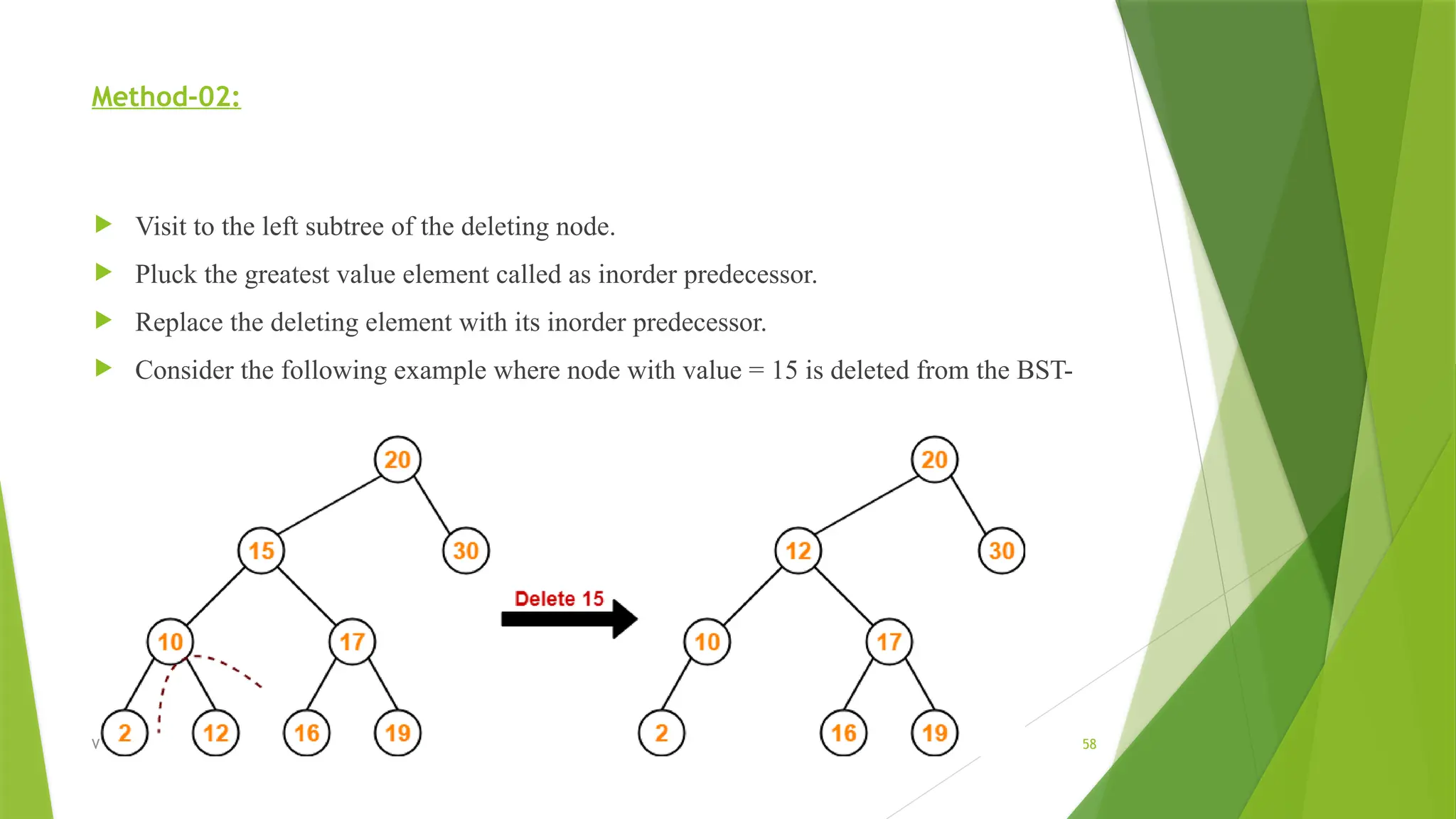
08/18/2025 VELAMMAL ENGINEERING COLLEGE, Dept. of CSE 57 Example  Consider the following example where node with value = 15 is deleted from the BST-

08/18/2025 VELAMMAL ENGINEERING COLLEGE, Dept. of CSE 58 Method-02:  Visit to the left subtree of the deleting node.  Pluck the greatest value element called as inorder predecessor.  Replace the deleting element with its inorder predecessor.  Consider the following example where node with value = 15 is deleted from the BST-

08/18/2025 VELAMMAL ENGINEERING COLLEGE, Dept. of CSE 59 Advantages of using binary search tree  Searching become very efficient in a binary search tree since, we get a hint at each step, about which sub-tree contains the desired element.  The binary search tree is considered as efficient data structure in compare to arrays and linked lists. In searching process, it removes half sub-tree at every step. Searching for an element in a binary search tree takes o(log2n) time. In worst case, the time it takes to search an element is 0(n).  It also speed up the insertion and deletion operations as compare to that in array and linked list.

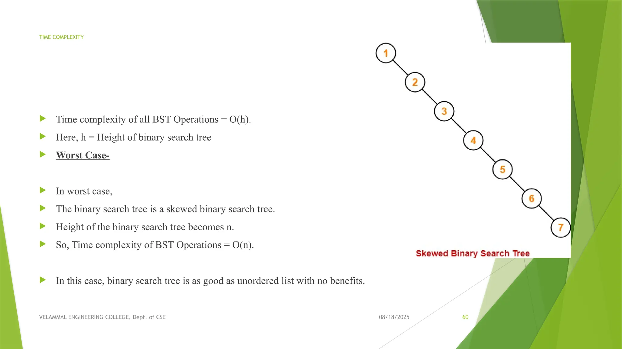
08/18/2025 VELAMMAL ENGINEERING COLLEGE, Dept. of CSE 60 TIME COMPLEXITY  Time complexity of all BST Operations = O(h).  Here, h = Height of binary search tree  Worst Case-  In worst case,  The binary search tree is a skewed binary search tree.  Height of the binary search tree becomes n.  So, Time complexity of BST Operations = O(n).  In this case, binary search tree is as good as unordered list with no benefits.

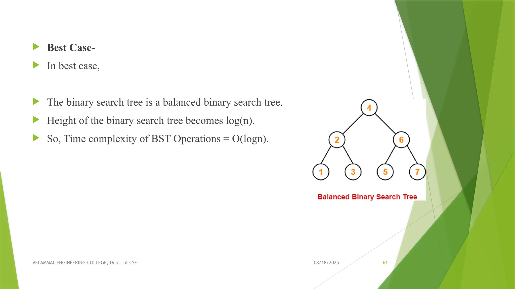
08/18/2025 VELAMMAL ENGINEERING COLLEGE, Dept. of CSE 61  Best Case-  In best case,  The binary search tree is a balanced binary search tree.  Height of the binary search tree becomes log(n).  So, Time complexity of BST Operations = O(logn).

08/18/2025 VELAMMAL ENGINEERING COLLEGE, Dept. of CSE 62 APPLICATIONS -BST 1) Used to express arithmetic expressions 2) Used to evaluate expression trees. 3) Used for indexing IP addresses. 4) It is used to implement dictionary. 5) It is used to implement multilevel indexing in DATABASE. 7) To implement Huffman Coding Algorithm. 8) It is used to implement searching Algorithm. 9) Implementing routing table in router.

08/18/2025 VELAMMAL ENGINEERING COLLEGE, Dept. of CSE 63 THANK YOU

Balanced Binaries – AVL Trees

Balanced Binaries – AVL Trees Height of a tree node: 1. The height of a node with no elements is 0 2. The height of a node with 1 element is 1 3. The height of a node with > 1 element is 1 + the height of its tallest subtree

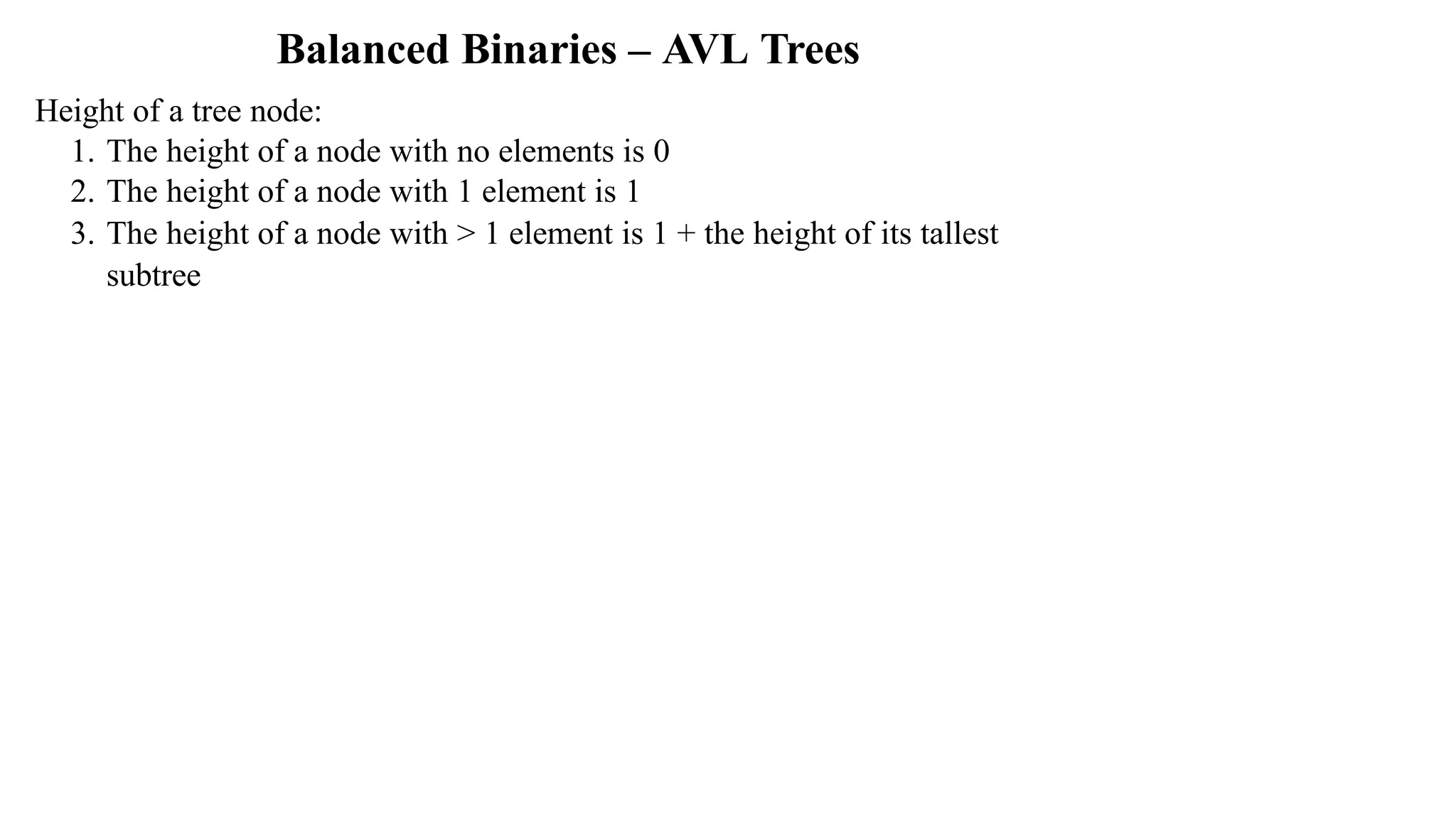
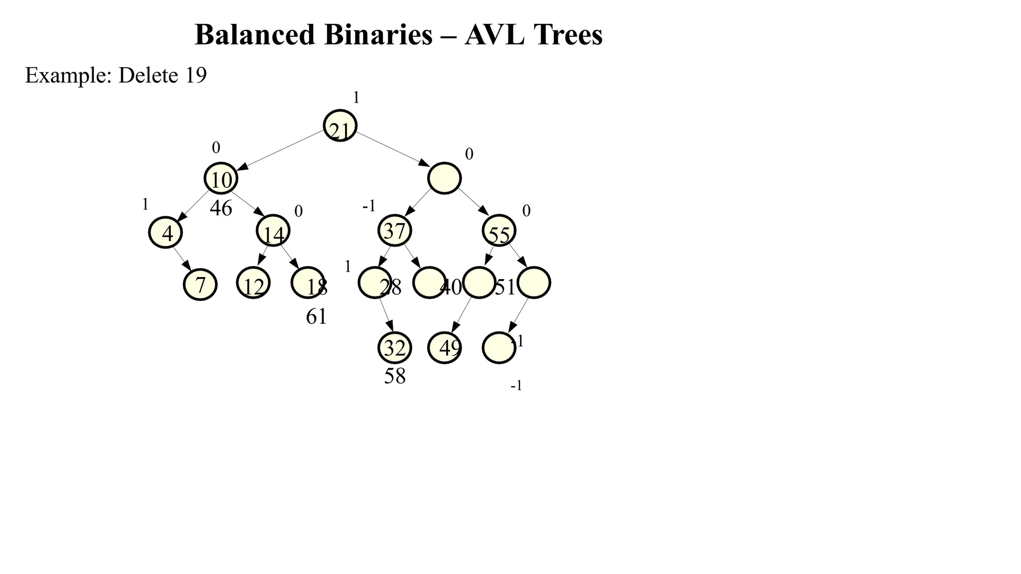
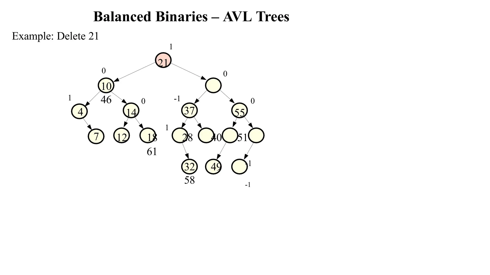
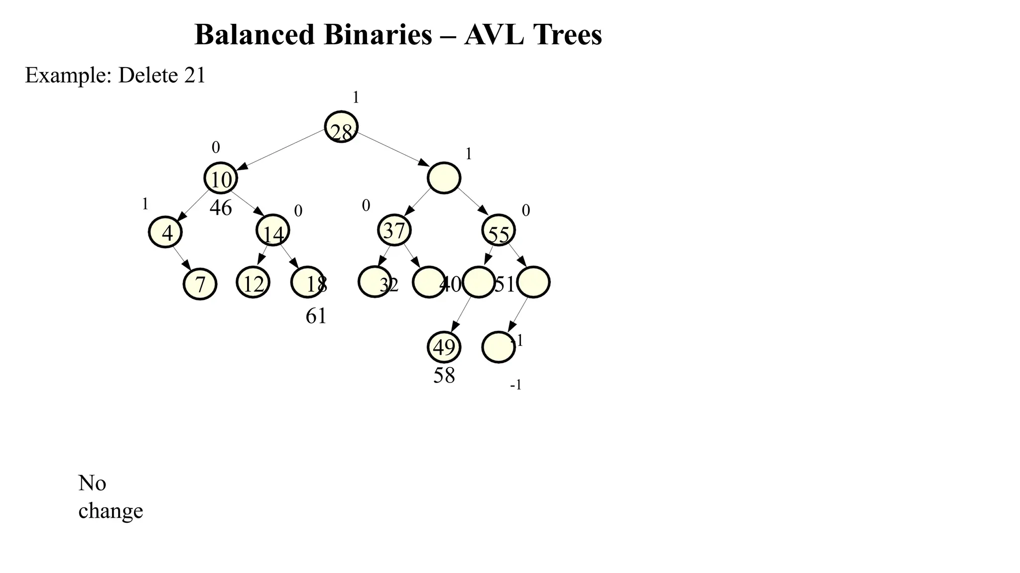
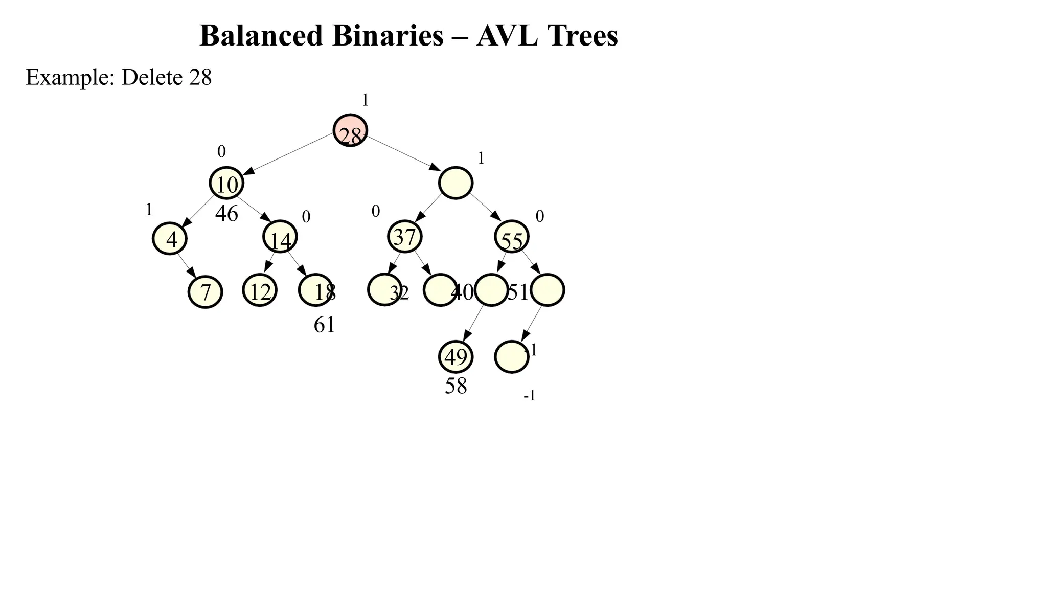
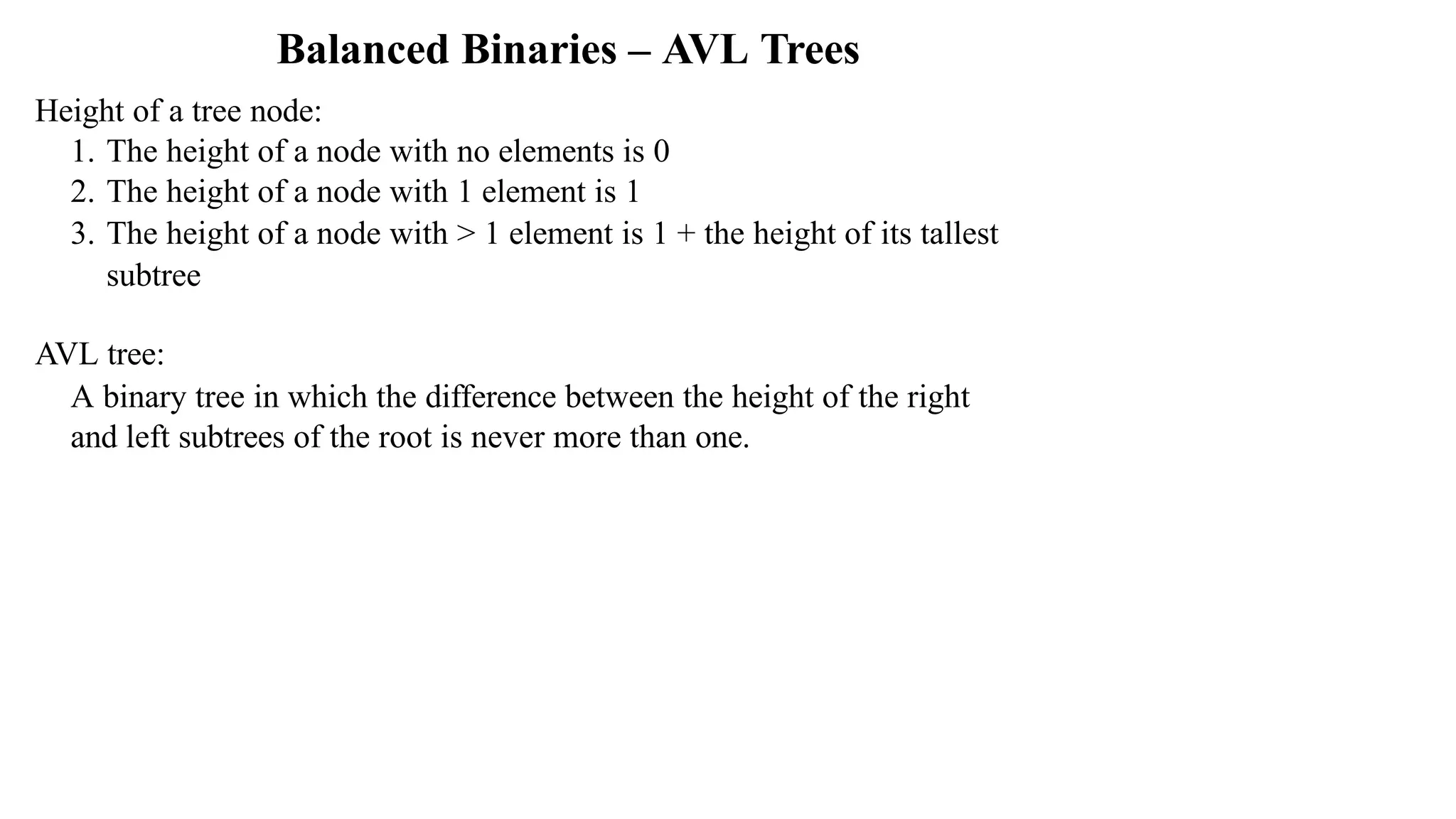
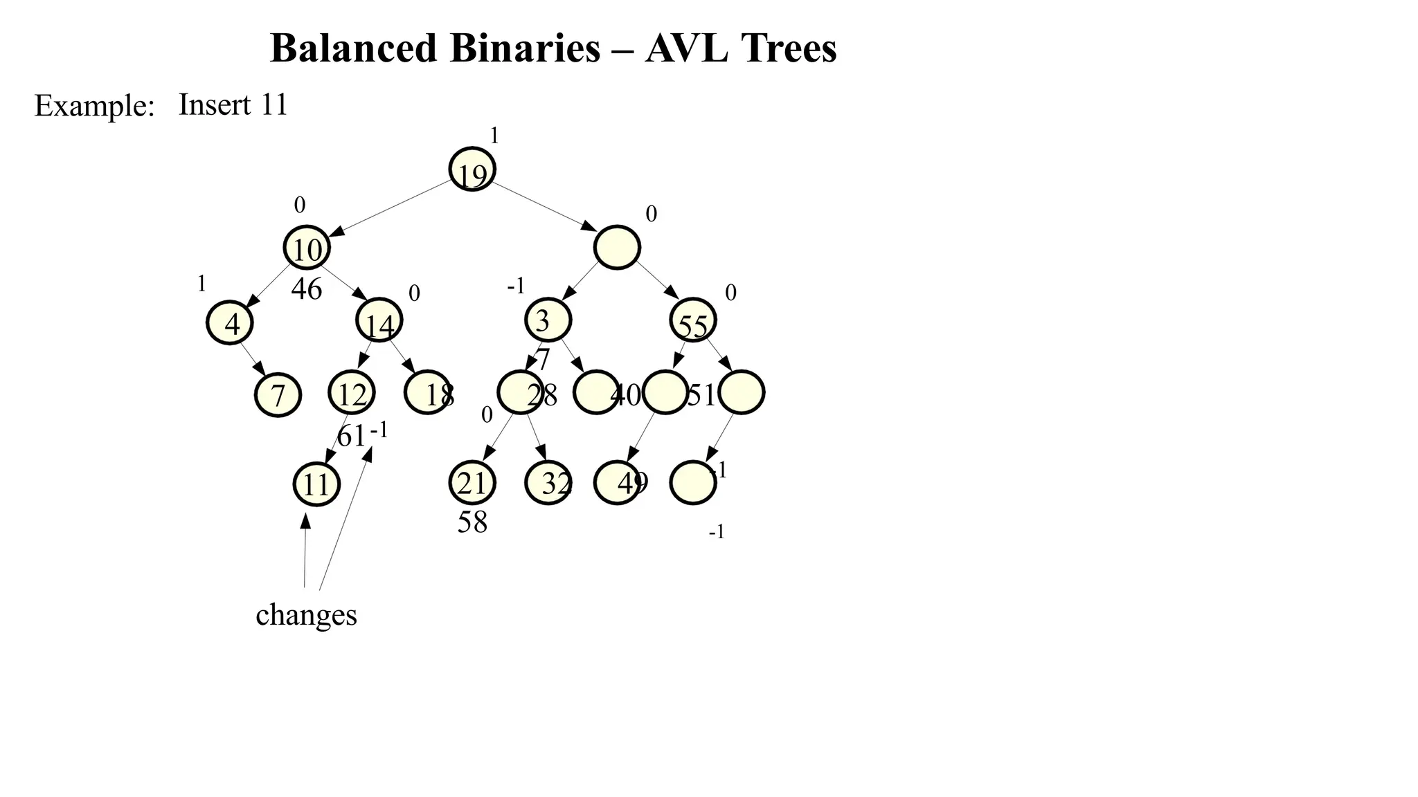
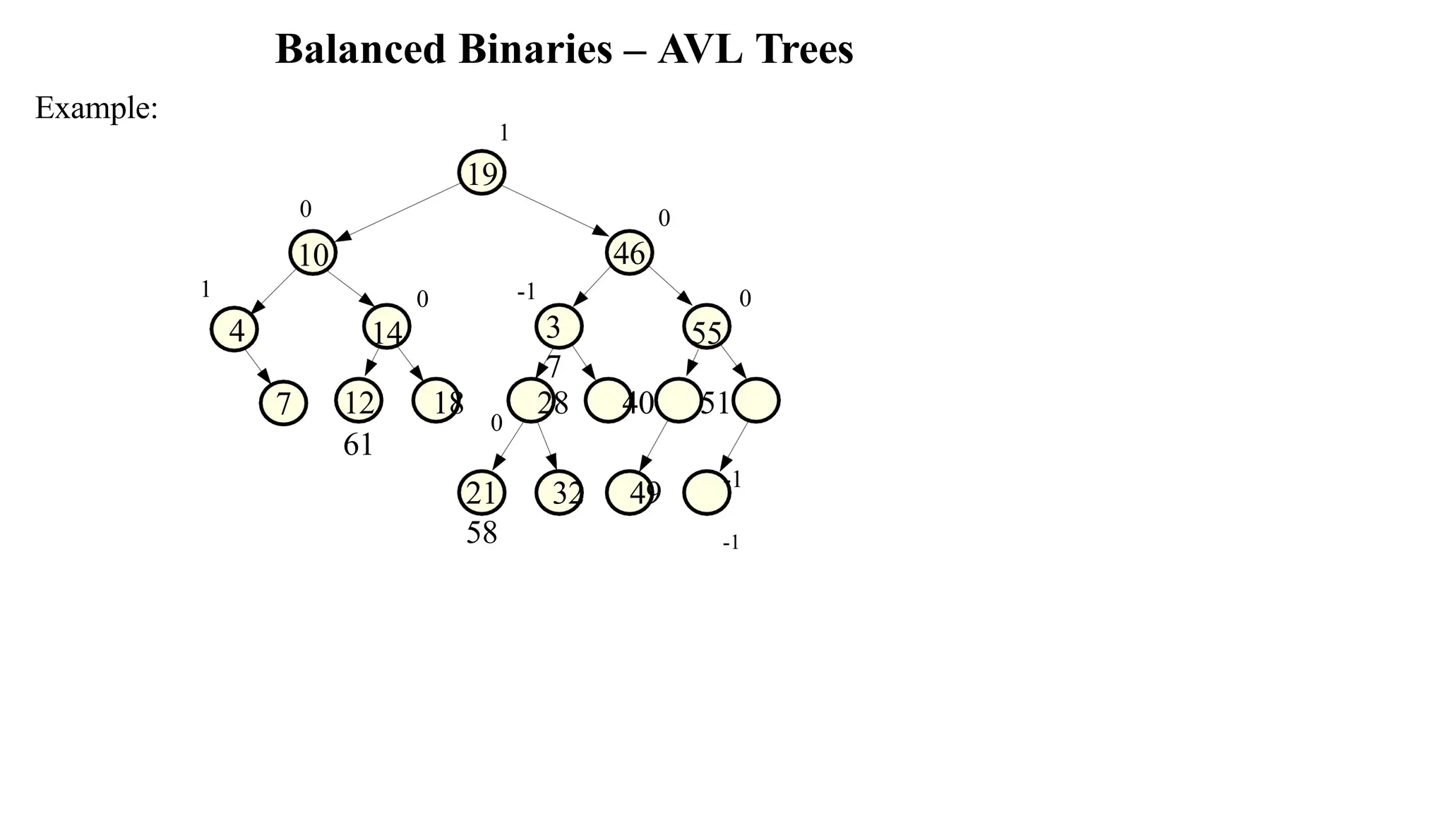
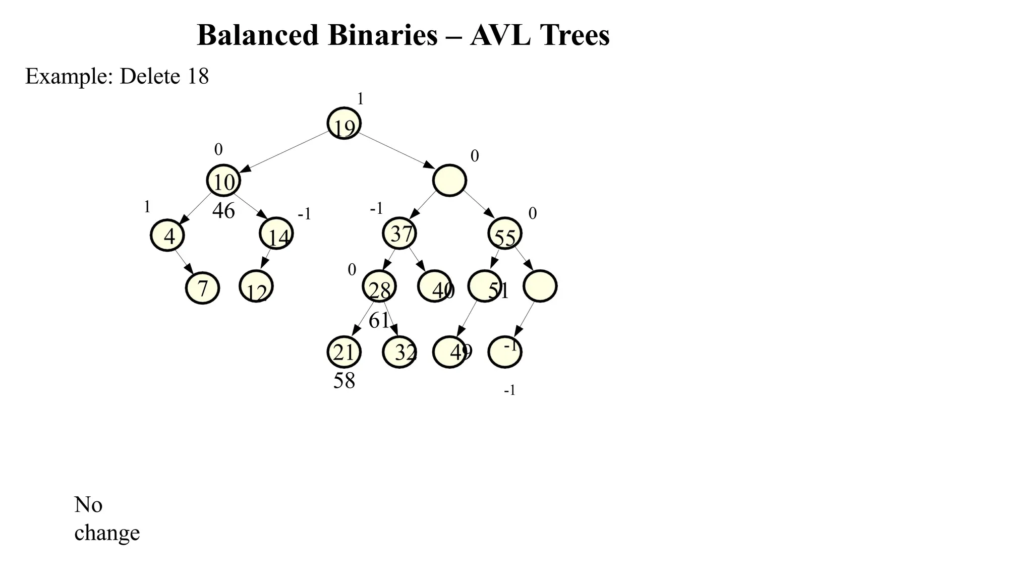
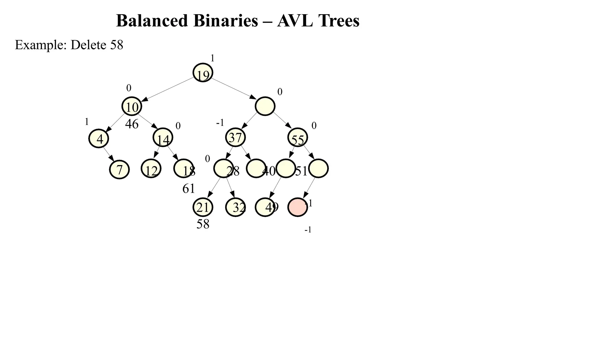
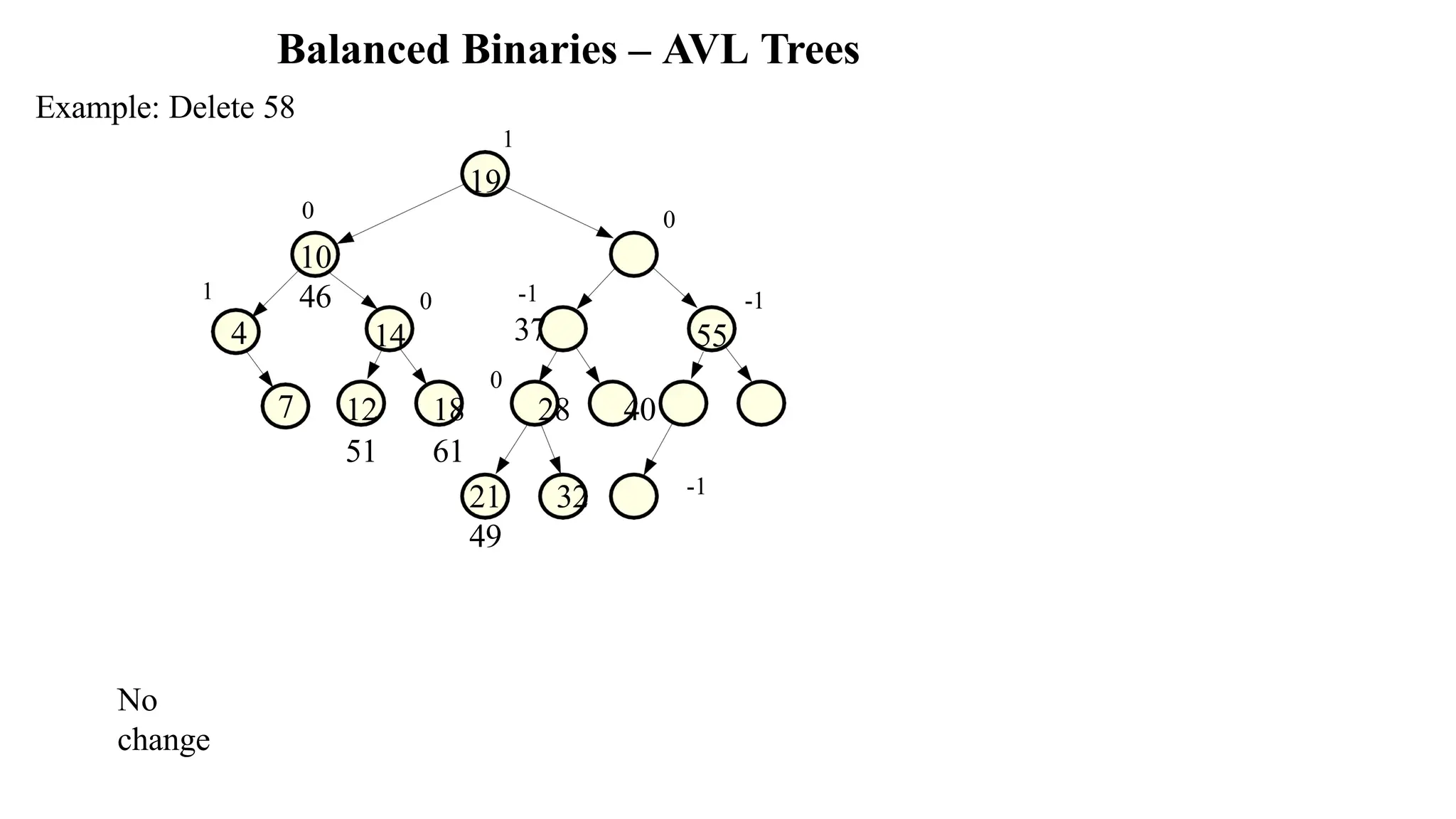
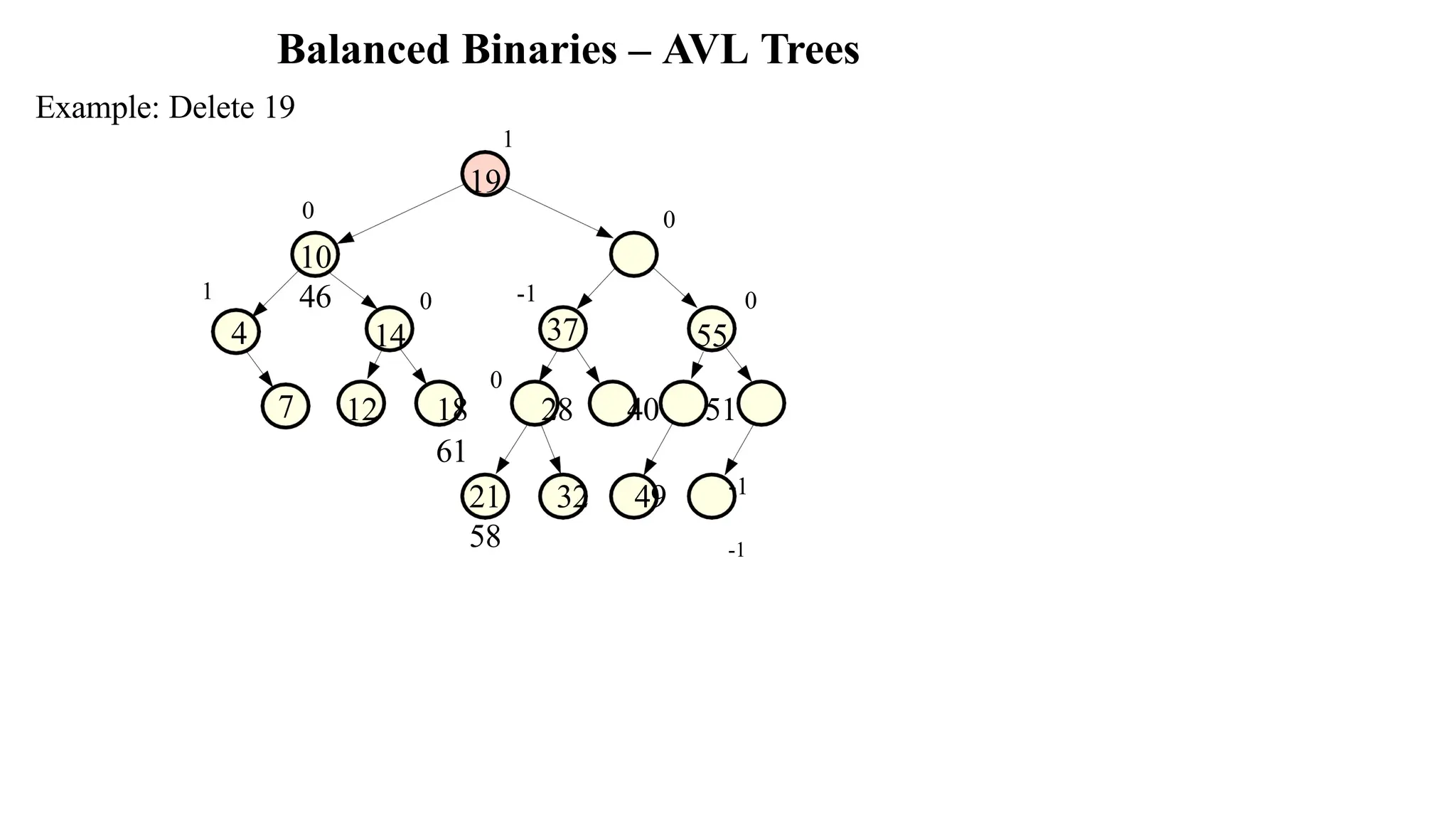
Balanced Binaries – AVL Trees Height of a tree node: 1. The height of a node with no elements is 0 2. The height of a node with 1 element is 1 3. The height of a node with > 1 element is 1 + the height of its tallest subtree AVL tree: A binary tree in which the difference between the height of the right and left subtrees of the root is never more than one.

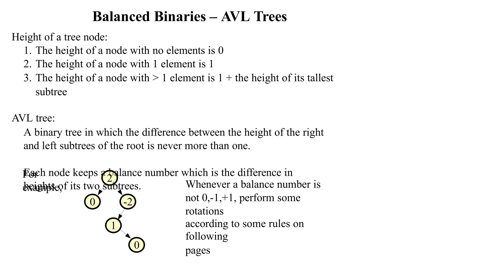
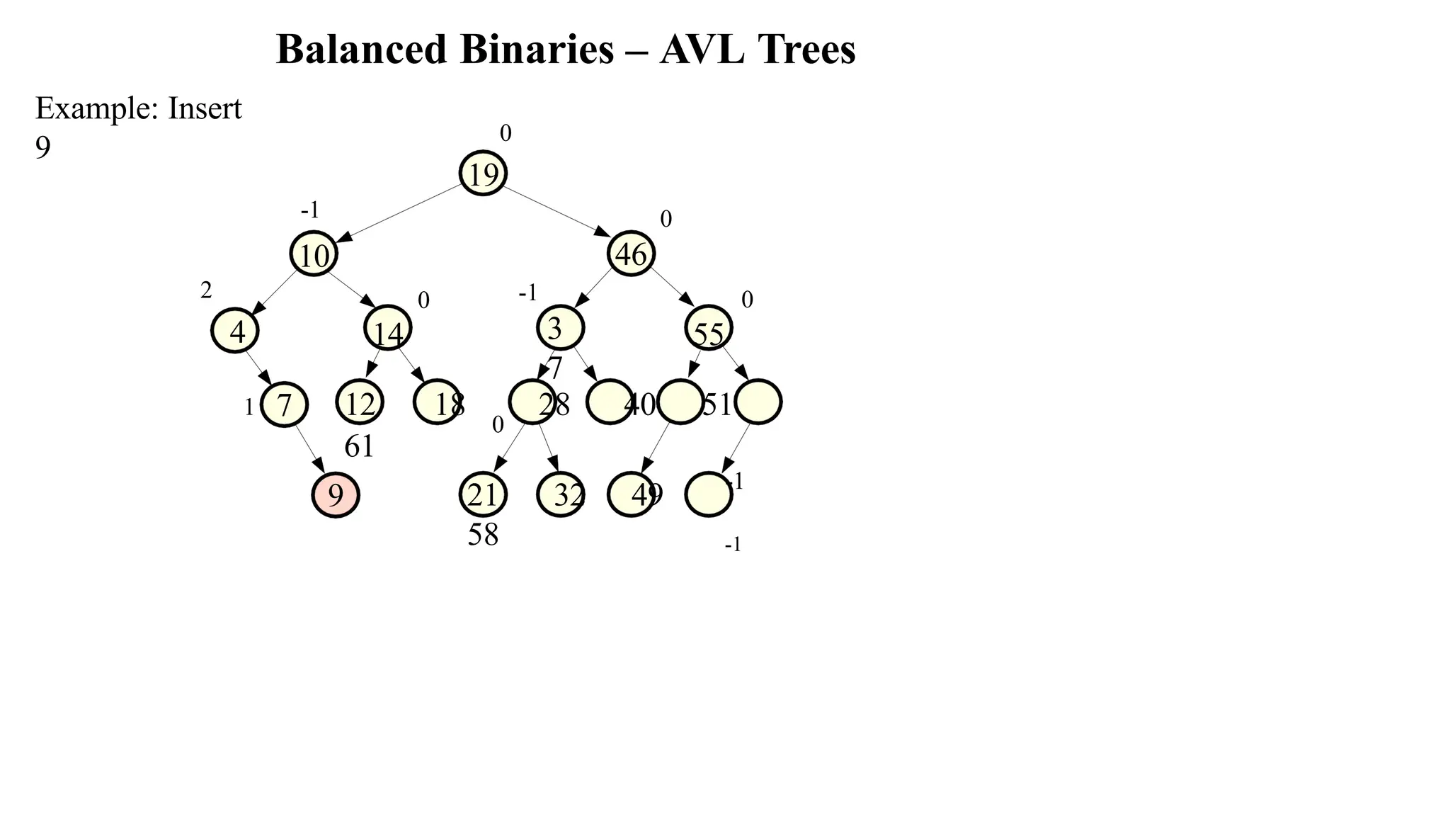
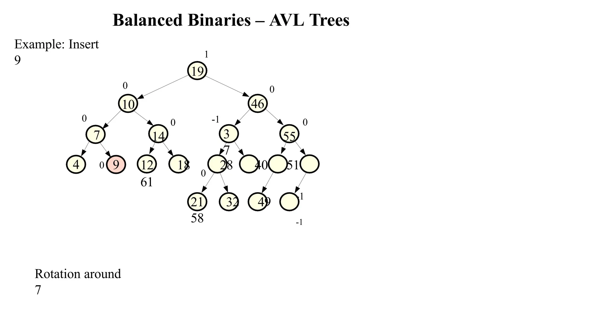
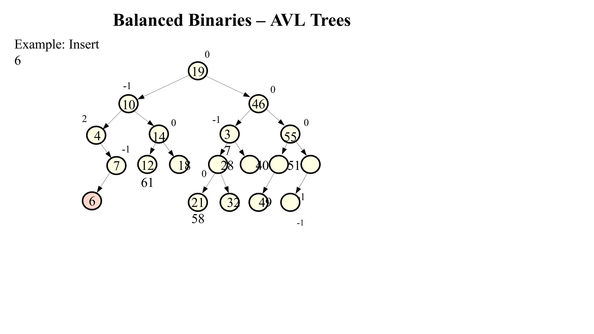
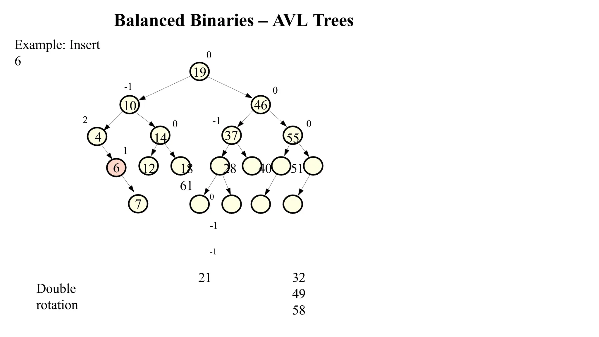
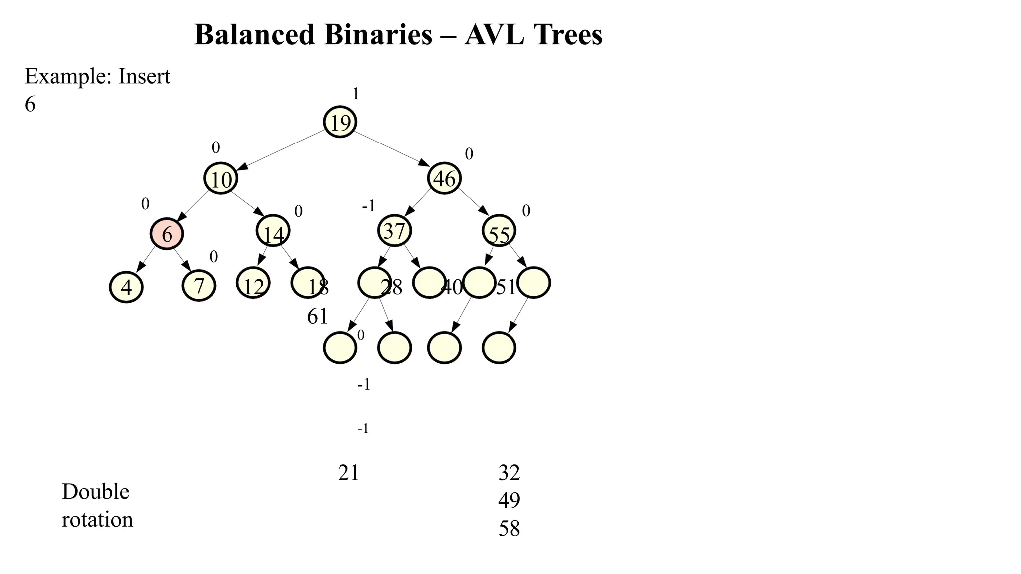
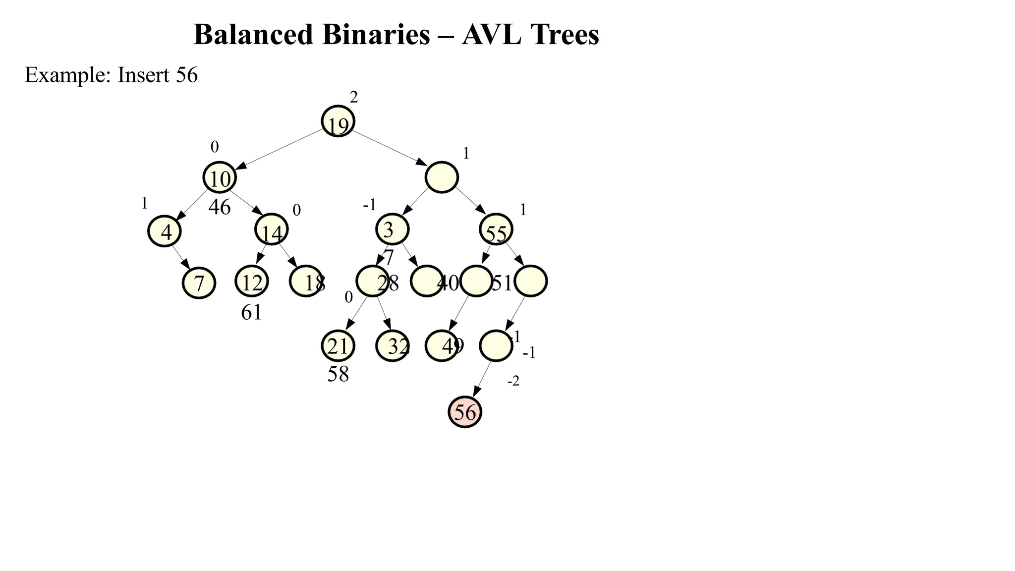
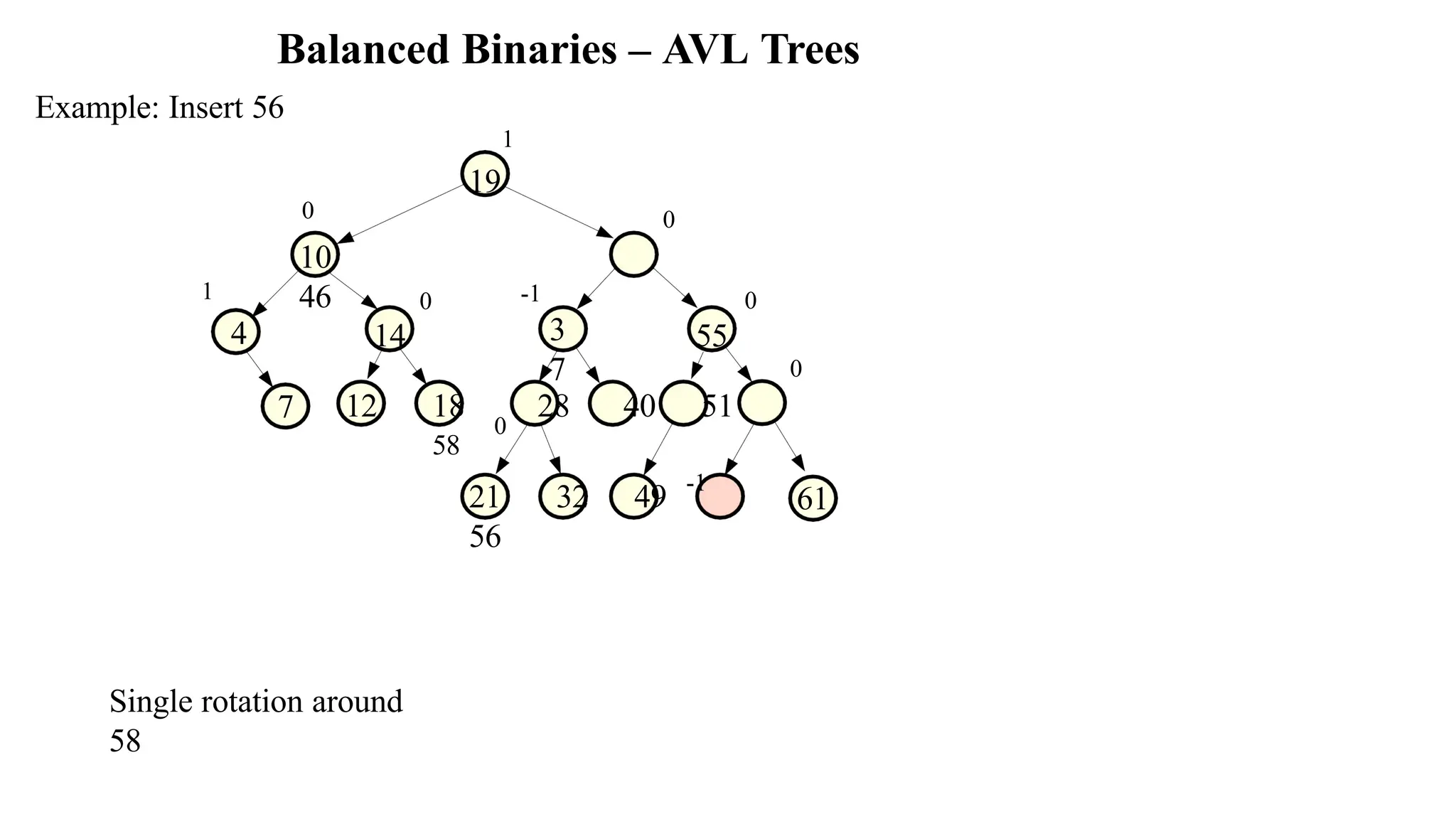
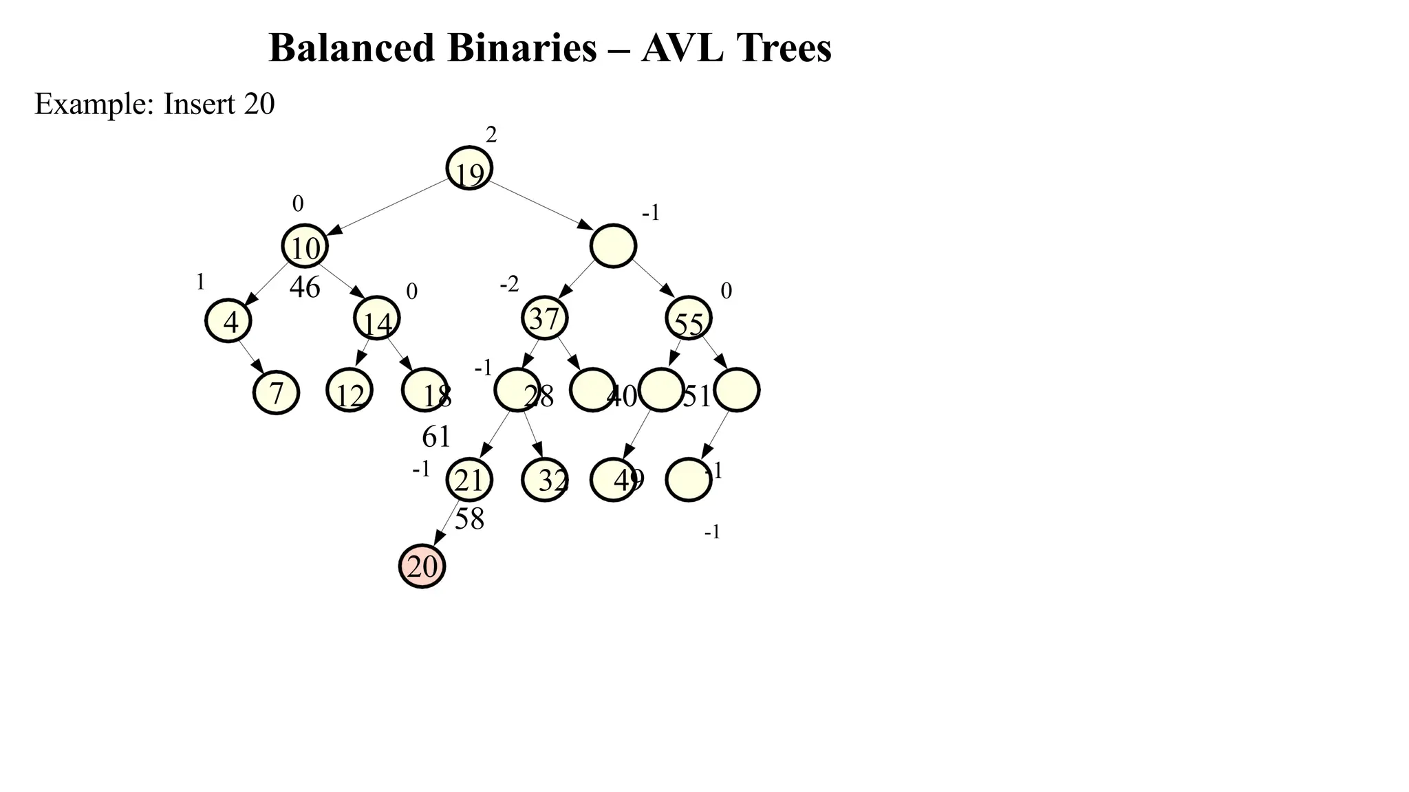
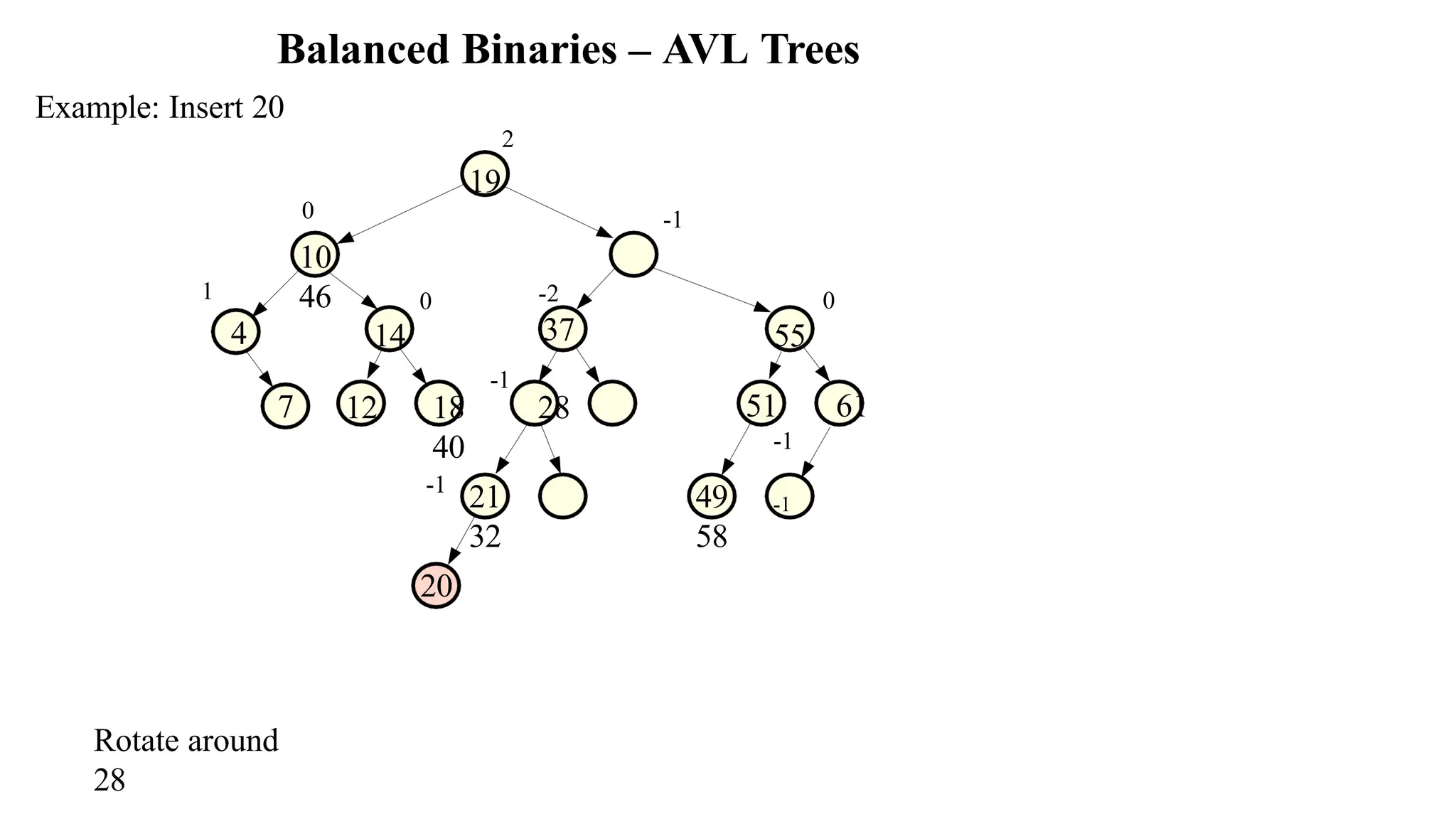
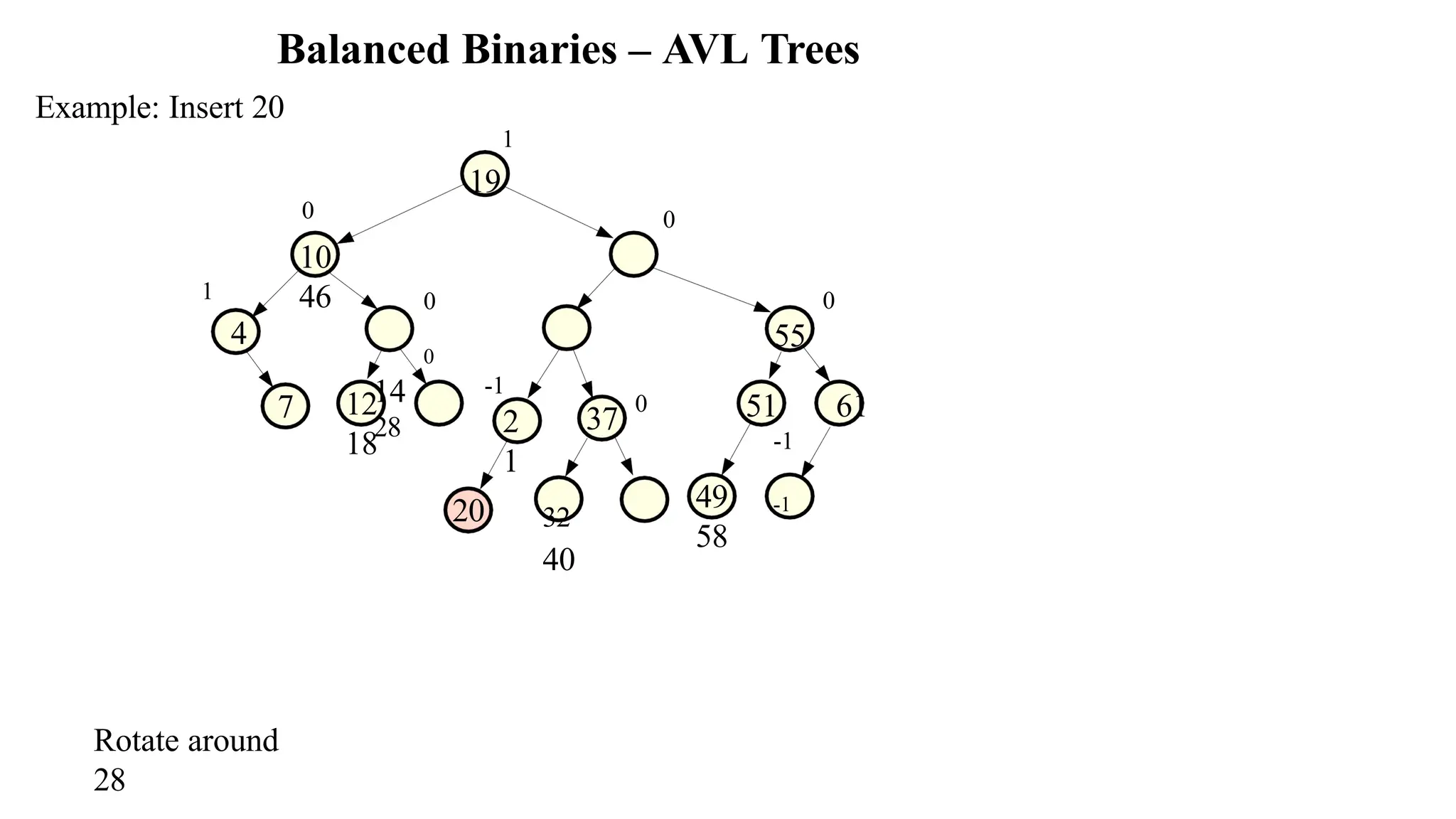
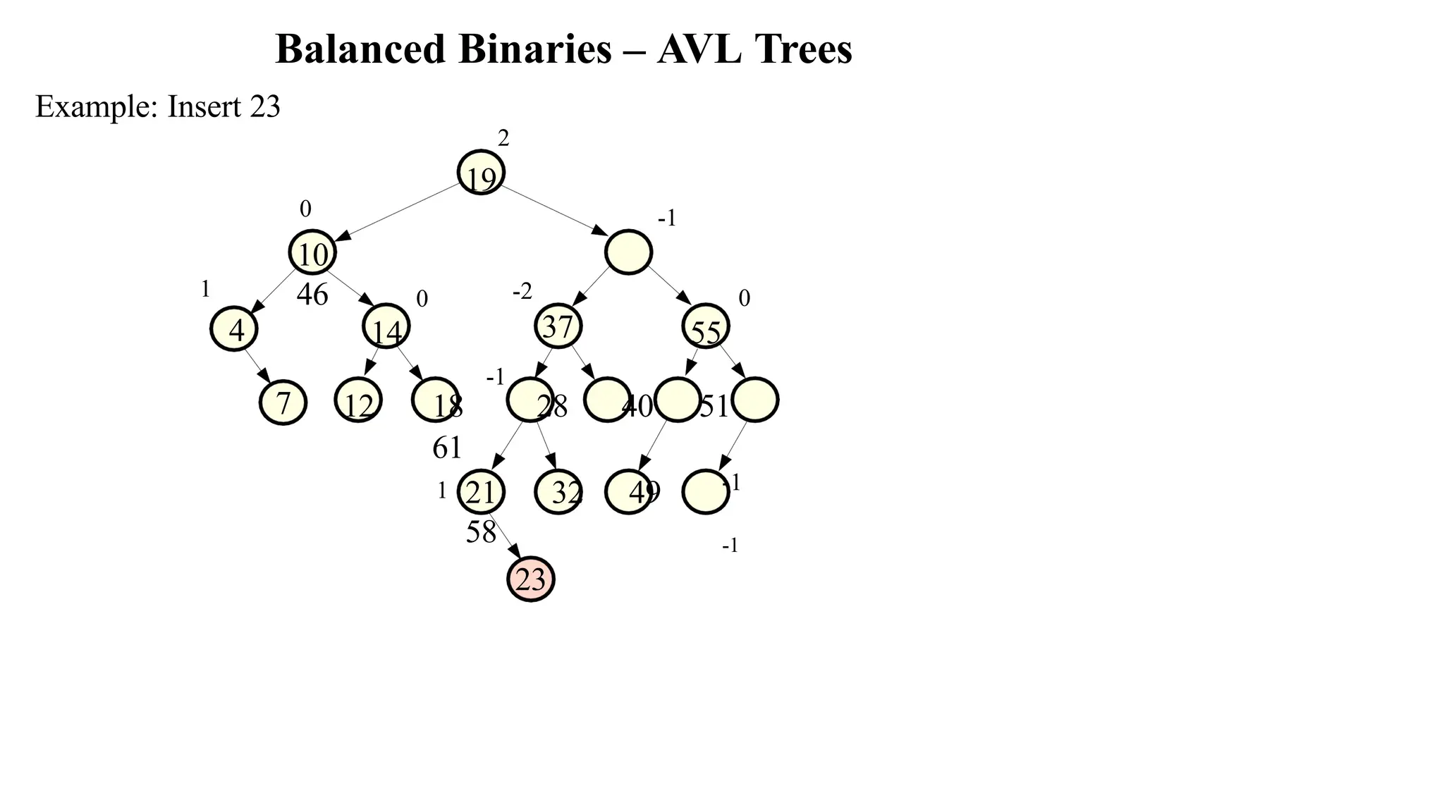
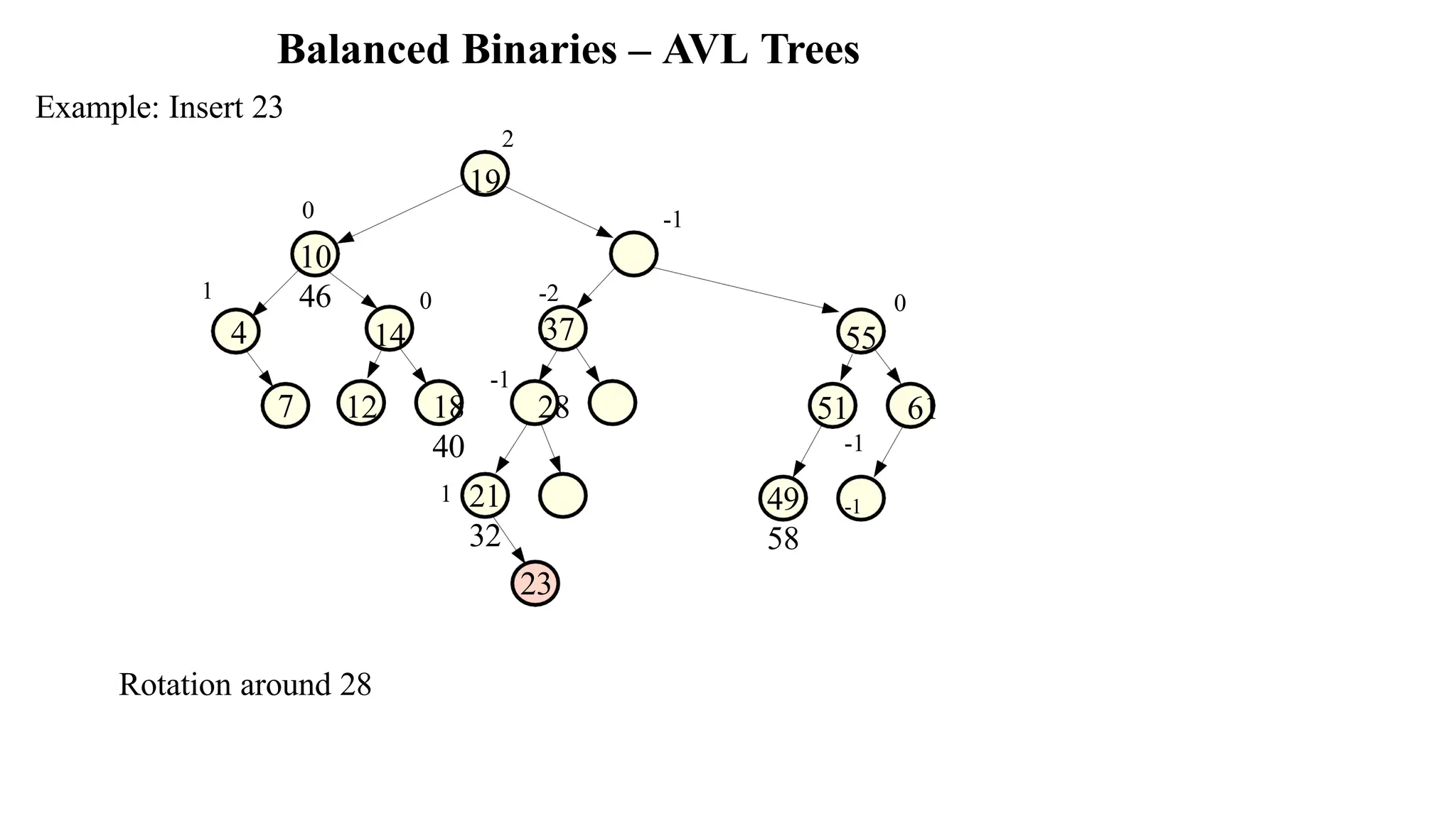
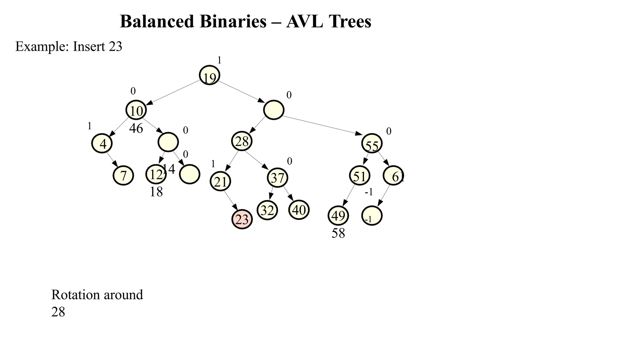
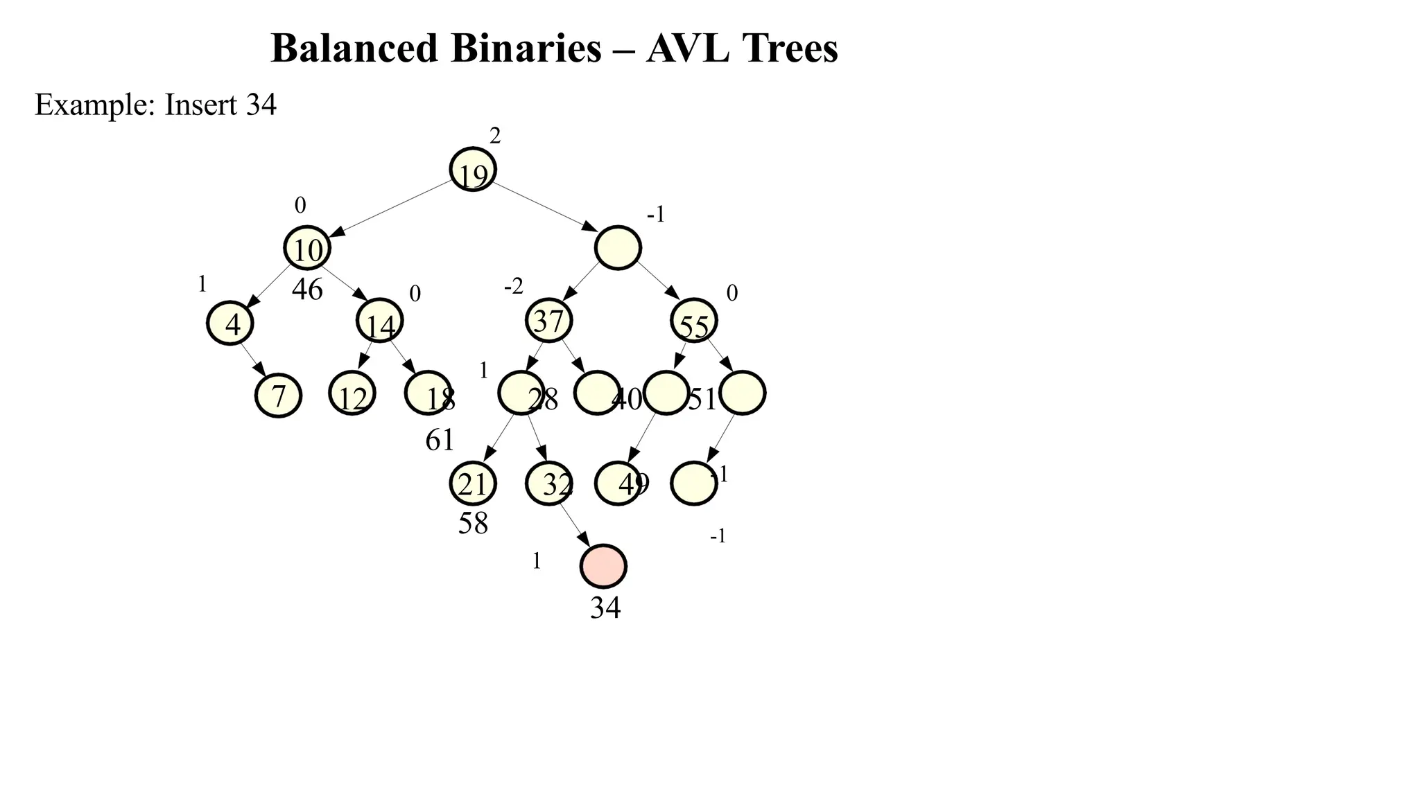
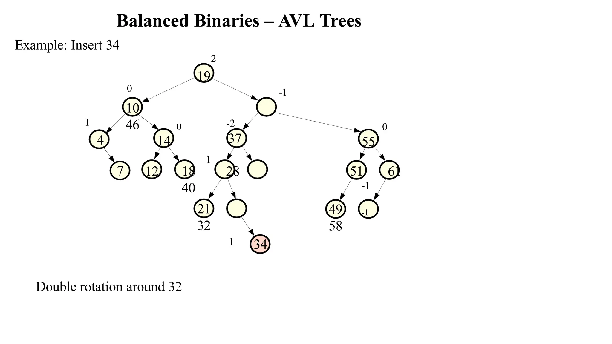
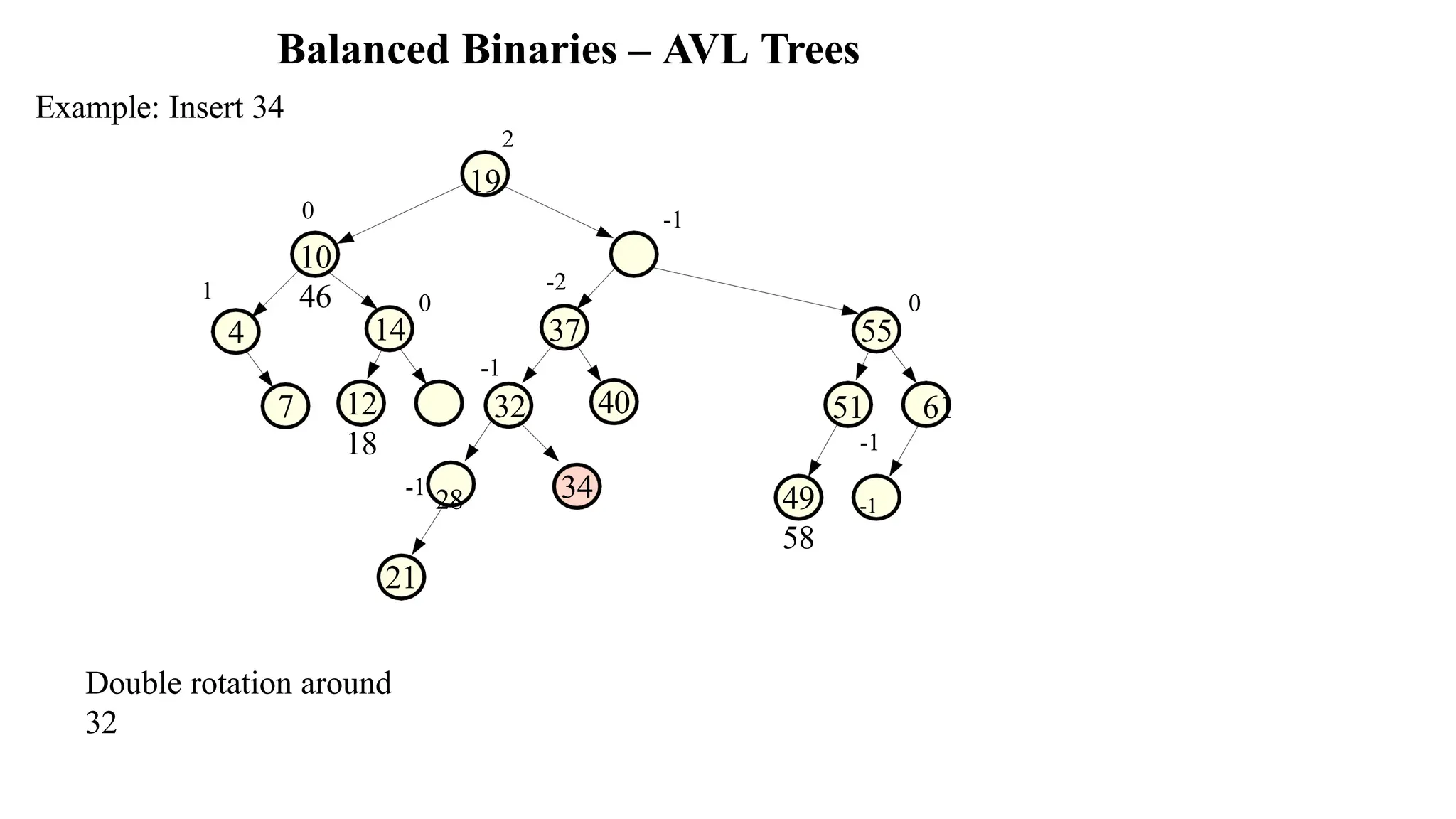
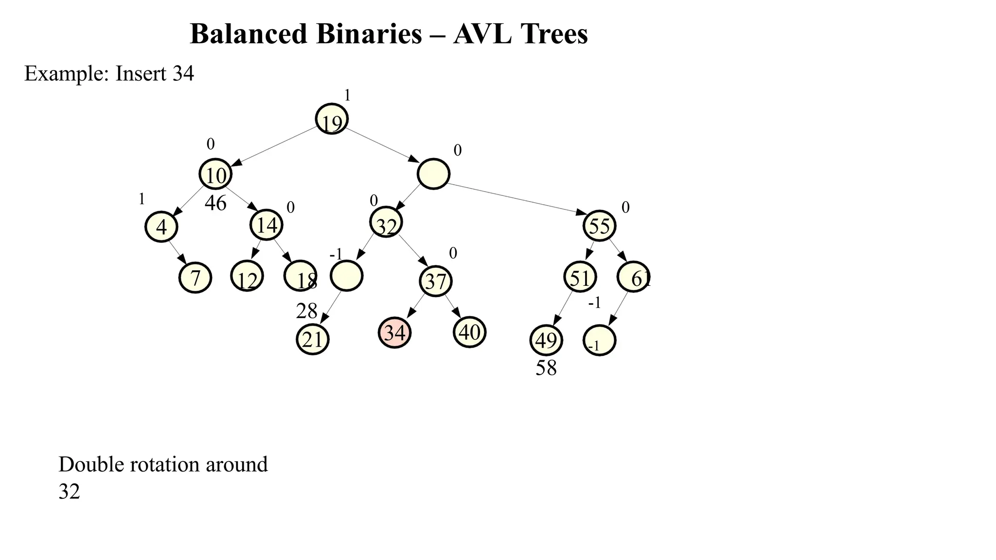
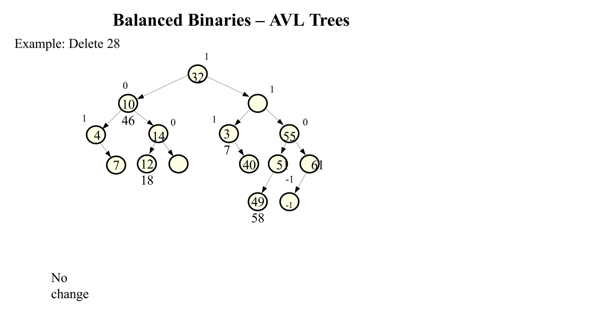
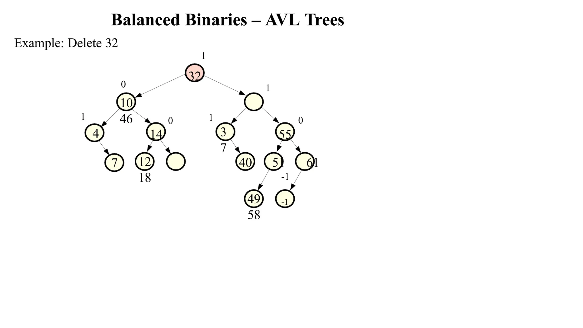
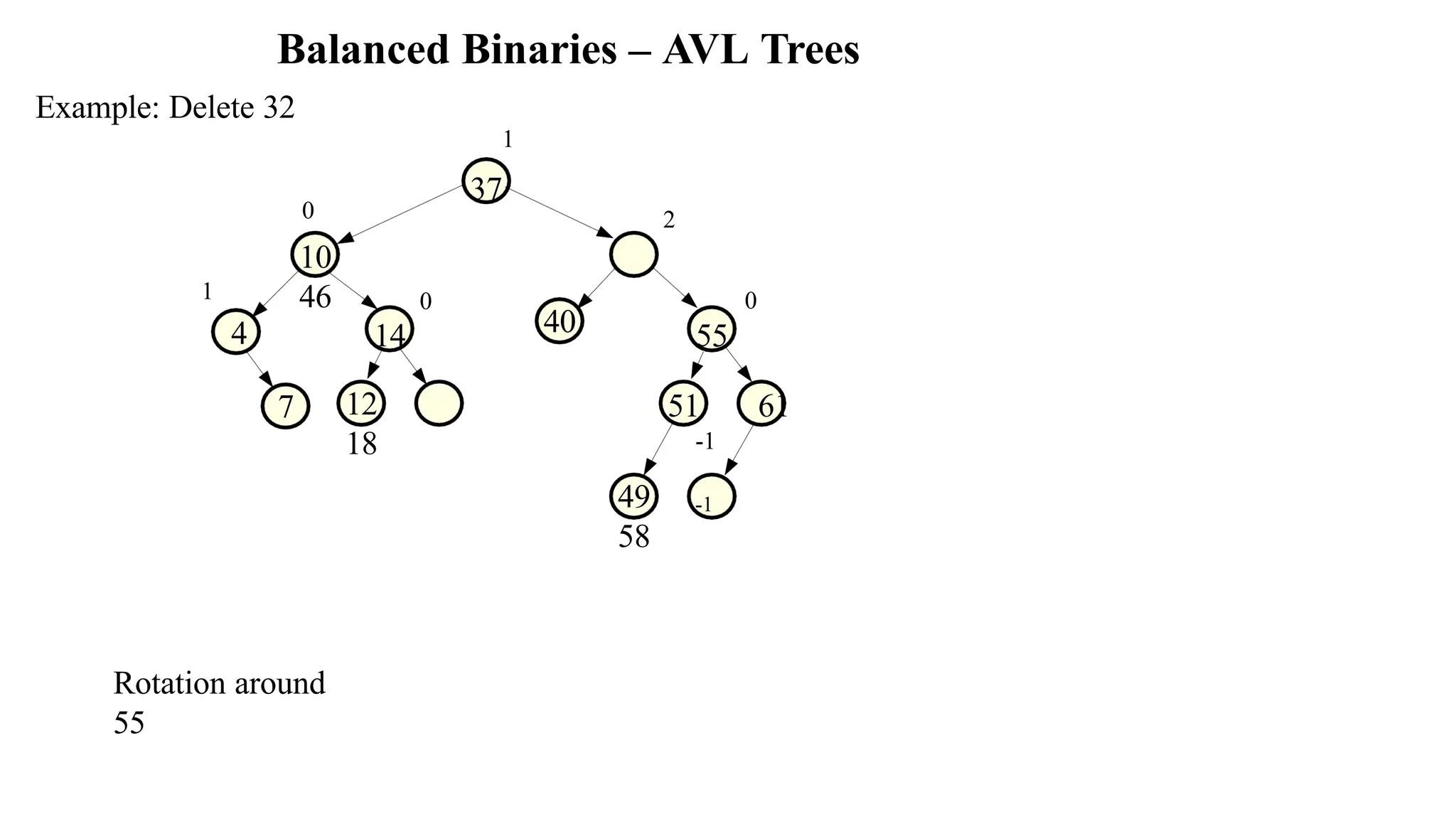
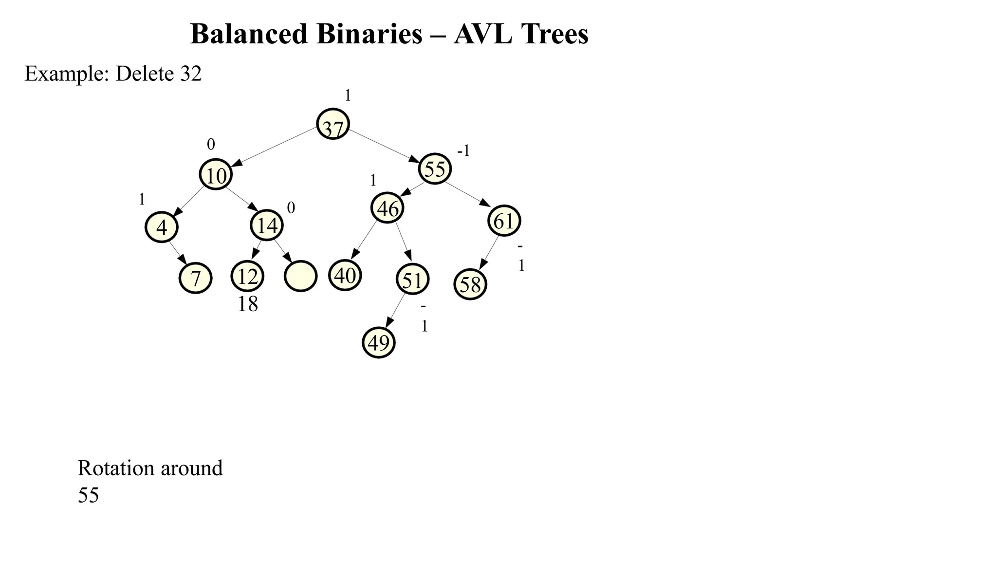
Balanced Binaries – AVL Trees Height of a tree node: 1. The height of a node with no elements is 0 2. The height of a node with 1 element is 1 3. The height of a node with > 1 element is 1 + the height of its tallest subtree AVL tree: A binary tree in which the difference between the height of the right and left subtrees of the root is never more than one. Each node keeps a balance number which is the difference in heights of its two subtrees. For example, 2 0 -2 1 0 Whenever a balance number is not 0,-1,+1, perform some rotations according to some rules on following pages

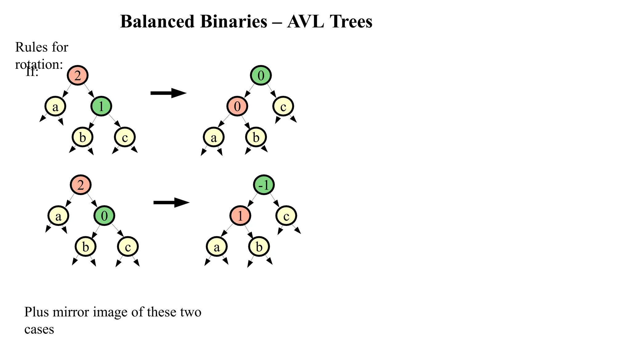
Balanced Binaries – AVL Trees Rules for rotation: If: 2 a 1 b c 0 c 0 b a 2 a 0 b c -1 c 1 b a Plus mirror image of these two cases

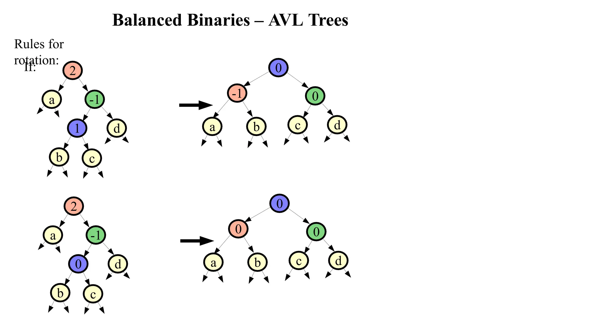
Balanced Binaries – AVL Trees Rules for rotation: If: 2 a -1 1 d c b 0 -1 0 c d b a 2 a -1 0 d c b 0 0 0 c d b a

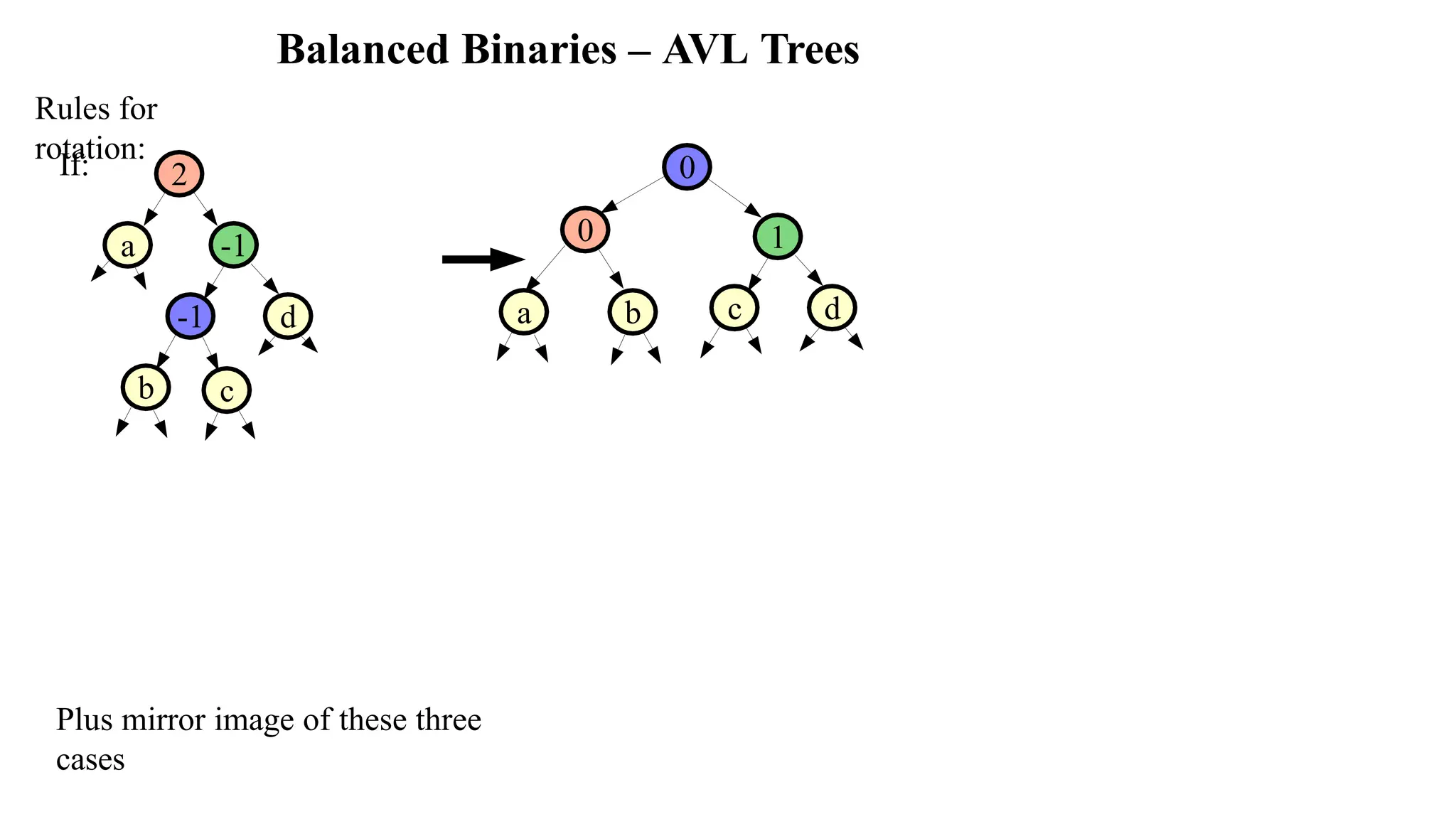
Balanced Binaries – AVL Trees Rules for rotation: If: 2 a -1 -1 d c b 0 0 1 c d b a Plus mirror image of these three cases

Balanced Binaries – AVL Trees Example: 46 21 32 49 58 7 -1 3 7 12 18 28 40 51 61 -1 -1 0 55 0 0 14 0 0 10 1 19 1 4

Balanced Binaries – AVL Trees Example: 21 32 49 58 7 -1 3 7 12 18 28 40 51 61 -1 -1 0 55 0 0 14 0 0 10 46 Insert 2 1 19 0 4 2 changes

Balanced Binaries – AVL Trees Example: 21 32 49 58 7 -1 3 7 12 18 28 40 51 61 -1 -1 0 55 0 0 14 0 0 10 46 Insert 11 1 19 1 4 11 changes -1

Balanced Binaries – AVL Trees Example: Insert 9 46 21 32 49 58 7 -1 3 7 12 18 28 40 51 61 -1 -1 0 55 0 0 14 0 -1 10 0 19 9 2 4 1

Balanced Binaries – AVL Trees Example: Insert 9 46 21 32 49 58 4 -1 3 7 12 18 28 40 51 61 -1 -1 0 55 0 0 14 0 0 10 1 19 9 0 7 0 Rotation around 7

Balanced Binaries – AVL Trees Example: Insert 6 46 21 32 49 58 7 -1 3 7 12 18 28 40 51 61 -1 -1 0 55 0 0 14 0 -1 10 0 19 2 4 6 -1

Balanced Binaries – AVL Trees Example: Insert 6 46 7 0 55 0 0 14 -1 37 12 18 28 40 51 61 0 -1 -1 21 32 49 58 -1 10 0 19 2 4 6 1 Double rotation

Balanced Binaries – AVL Trees Example: Insert 6 46 4 7 0 55 0 0 14 -1 37 12 18 28 40 51 61 0 -1 -1 21 32 49 58 0 10 1 19 0 6 0 Double rotation

Balanced Binaries – AVL Trees 21 32 49 58 7 -1 3 7 12 18 28 40 51 61 -1 -2 1 55 1 0 14 0 0 10 46 Example: Insert 56 2 19 1 4 56 -1

Balanced Binaries – AVL Trees 61 7 -1 3 7 12 18 28 40 51 58 -1 0 0 55 0 0 14 0 0 10 46 Example: Insert 56 1 19 1 4 21 32 49 56 Single rotation around 58

Balanced Binaries – AVL Trees Example: 46 21 32 49 58 7 -1 3 7 12 18 28 40 51 61 -1 -1 0 55 0 0 14 0 10 1 19 1 4 0

Balanced Binaries – AVL Trees 21 32 49 58 7 -2 37 12 18 28 40 51 61 -1 -1 0 55 -1 0 14 -1 0 10 46 Example: Insert 20 2 19 1 4 20 -1

Balanced Binaries – AVL Trees 49 58 21 32 7 -2 37 12 18 28 40 51 61 -1 -1 0 55 -1 0 14 -1 0 10 46 Example: Insert 20 2 19 1 4 20 -1 Rotate around 28

Balanced Binaries – AVL Trees 37 12 18 49 58 32 40 7 51 61 -1 -1 0 55 0 0 0 14 28 0 10 46 Example: Insert 20 1 19 1 4 20 -1 2 1 Rotate around 28 0

Balanced Binaries – AVL Trees Example: 46 21 32 49 58 7 -1 37 12 18 28 40 51 61 -1 -1 0 55 0 0 14 0 10 1 19 1 4 0

Balanced Binaries – AVL Trees 21 32 49 58 7 -2 37 12 18 28 40 51 61 -1 -1 0 55 -1 0 14 0 10 46 Example: Insert 23 2 19 1 4 -1 23 1

Balanced Binaries – AVL Trees 49 58 21 32 7 -2 37 12 18 28 40 51 61 -1 -1 0 55 -1 0 14 0 10 46 Example: Insert 23 2 19 1 4 -1 1 23 Rotation around 28

Balanced Binaries – AVL Trees 37 28 40 12 18 49 58 32 7 0 51 61 -1 -1 0 55 0 0 10 46 Example: Insert 23 1 19 1 4 0 0 14 23 1 21 Rotation around 28

Balanced Binaries – AVL Trees 7 -2 37 12 18 28 40 51 61 -1 -1 0 55 -1 0 14 0 10 46 Example: Insert 34 2 19 1 4 1 21 32 49 58 1 34

Balanced Binaries – AVL Trees 49 58 7 -2 37 12 18 28 40 51 61 -1 -1 0 55 -1 0 14 0 10 46 Example: Insert 34 2 19 1 4 1 21 32 1 34 Double rotation around 32

Balanced Binaries – AVL Trees 55 40 14 12 18 49 58 4 7 -2 37 51 61 -1 -1 0 -1 0 0 10 46 Example: Insert 34 2 19 1 -1 28 34 -1 32 21 Double rotation around 32

Balanced Binaries – AVL Trees 55 37 40 14 49 58 21 4 7 0 51 61 -1 -1 0 0 0 0 10 46 Example: Insert 34 1 19 1 -1 12 18 28 34 0 32 Double rotation around 32

Balanced Binaries – AVL Trees 21 32 49 58 7 -1 37 12 18 28 40 51 61 -1 -1 0 55 0 0 14 0 10 46 Example: Delete 18 1 19 1 4 0

Balanced Binaries – AVL Trees 21 32 49 58 7 -1 37 28 40 51 61 -1 -1 0 55 0 -1 14 12 0 10 46 Example: Delete 18 1 19 1 4 0 No change

Balanced Binaries – AVL Trees 21 32 49 7 -1 37 12 18 28 40 51 61 -1 -1 55 0 0 14 0 10 46 Example: Delete 58 1 19 1 4 0 No change

Balanced Binaries – AVL Trees 32 49 58 7 -1 37 12 18 28 40 51 61 -1 -1 0 55 0 0 14 0 10 46 Example: Delete 19 1 21 1 4 1

Balanced Binaries – AVL Trees 32 49 58 7 -1 37 12 18 28 40 51 61 -1 -1 0 55 0 0 14 0 10 46 Example: Delete 21 1 21 1 4 1

Balanced Binaries – AVL Trees 49 58 7 0 37 12 18 32 40 51 61 -1 -1 0 55 1 0 14 0 10 46 Example: Delete 21 1 28 1 4 No change

Balanced Binaries – AVL Trees 49 58 7 0 37 12 18 32 40 51 61 -1 -1 0 55 1 0 14 0 10 46 Example: Delete 28 1 28 1 4

Balanced Binaries – AVL Trees 12 18 49 58 7 1 3 7 40 51 61 -1 -1 0 55 1 0 14 0 10 46 Example: Delete 28 1 32 1 4 No change

Balanced Binaries – AVL Trees 12 18 49 58 7 1 3 7 40 51 61 -1 -1 0 55 1 0 14 0 10 46 Example: Delete 32 1 32 1 4

Balanced Binaries – AVL Trees 40 12 18 49 58 7 51 61 -1 -1 0 55 2 0 14 0 10 46 Example: Delete 32 1 37 1 4 Rotation around 55

Balanced Binaries – AVL Trees 55 40 14 12 18 49 58 4 7 51 - 1 61 - 1 -1 1 46 0 0 10 Example: Delete 32 1 37 1 Rotation around 55

AVL VELAMMAL ENGINEERING COLLEGE An Autonomous Institution, Affiliated to Anna University Chennai, & Approved by AICTE Delhi

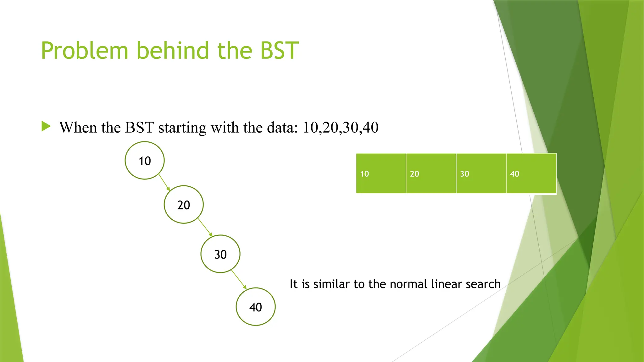
Problem behind the BST  When the BST starting with the data: 10,20,30,40 10 20 30 40 10 20 30 40 It is similar to the normal linear search

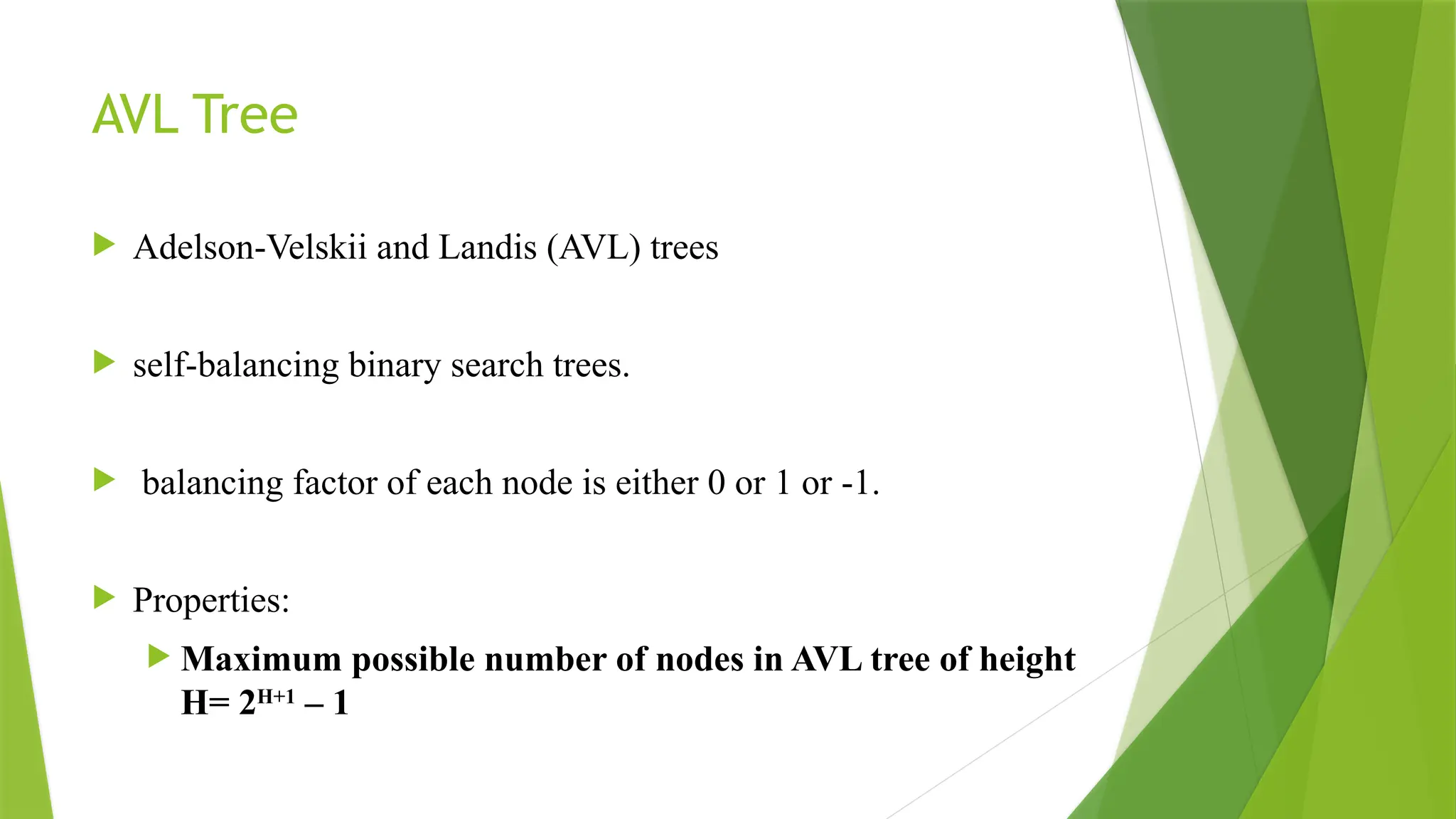
AVL Tree  Adelson-Velskii and Landis (AVL) trees  self-balancing binary search trees.  balancing factor of each node is either 0 or 1 or -1.  Properties:  Maximum possible number of nodes in AVL tree of height H= 2H+1 – 1

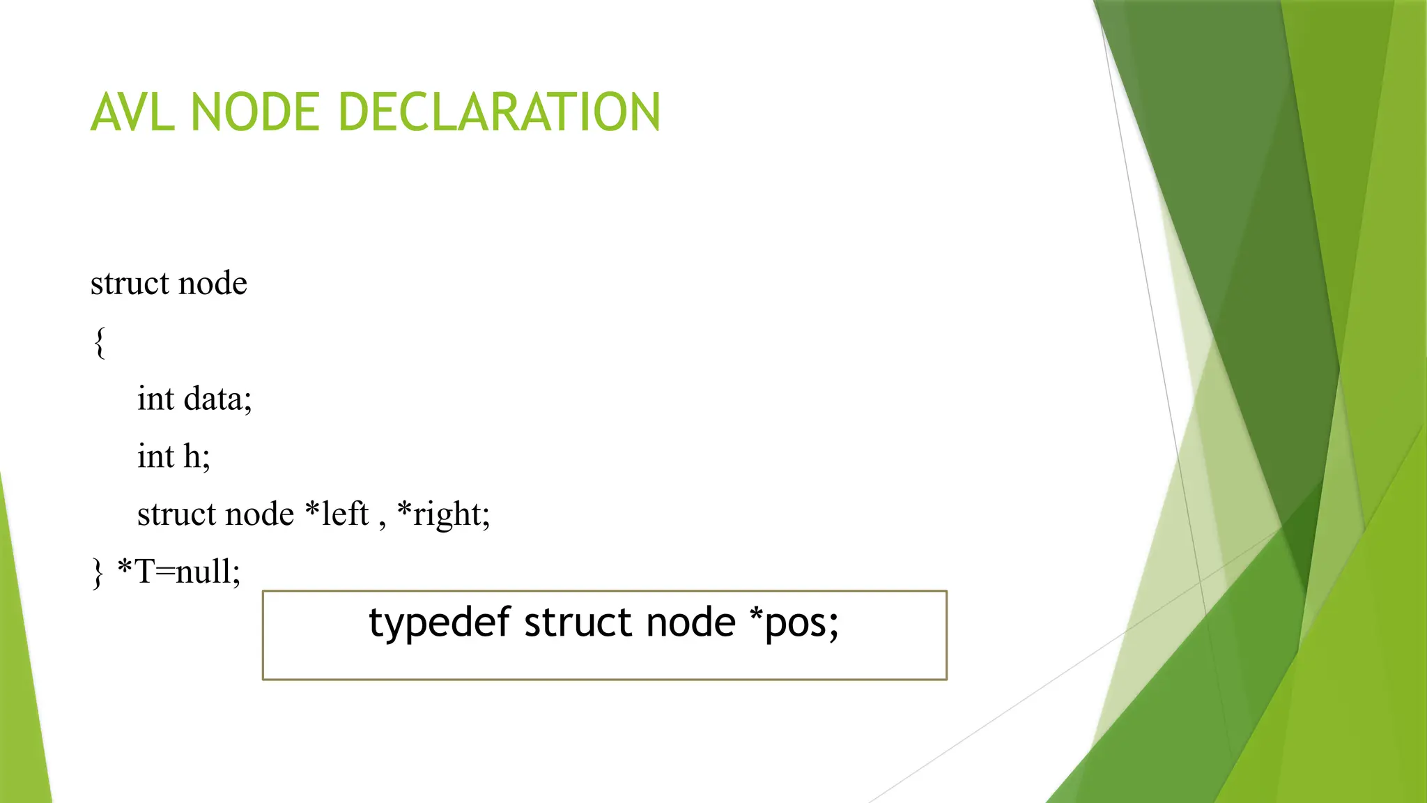
AVL NODE DECLARATION struct node { int data; int h; struct node *left , *right; } *T=null; typedef struct node *pos;

To calculate Height int height(pos p) { if(p==NULL) return -1; else return p->h; }

Single Rotation With Left (Right Rotation)  Imbalance occur when inserting at Left of Left sub tree,

RR Routine pos SRWL(pos k2) { pos k1; k1=k2->left; k2->left=k1->right; k1->right=k2; k2->h=1+max(height(k2->left),height(k2->right)); k1->h=1+max(height(k1->left),k2->h); return k1; }

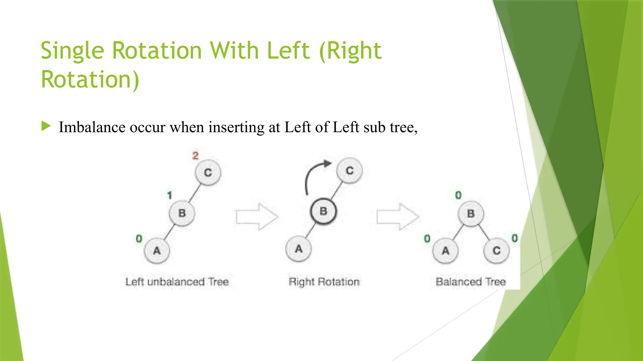
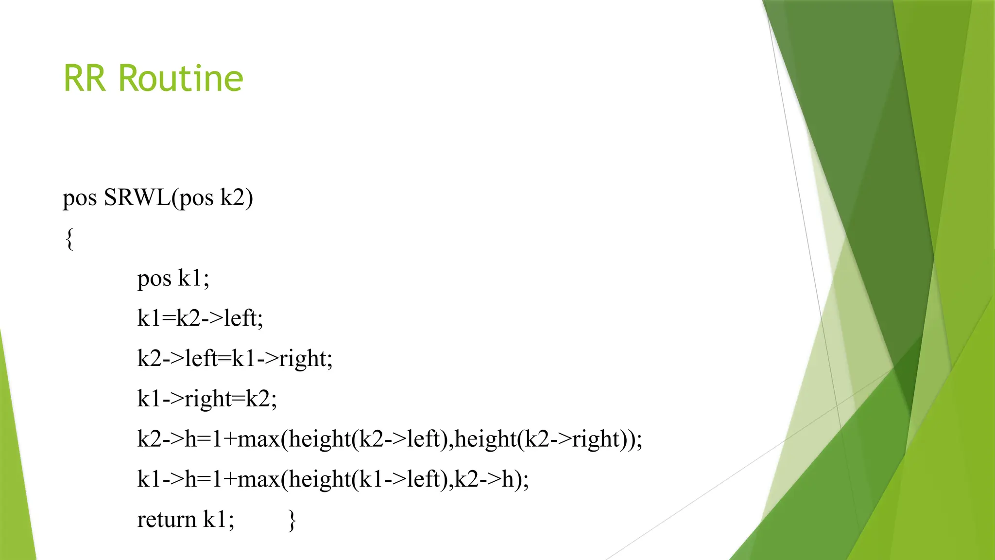
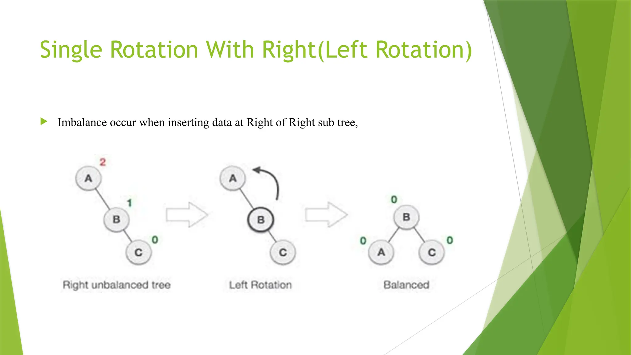
Single Rotation With Right(Left Rotation)  Imbalance occur when inserting data at Right of Right sub tree,

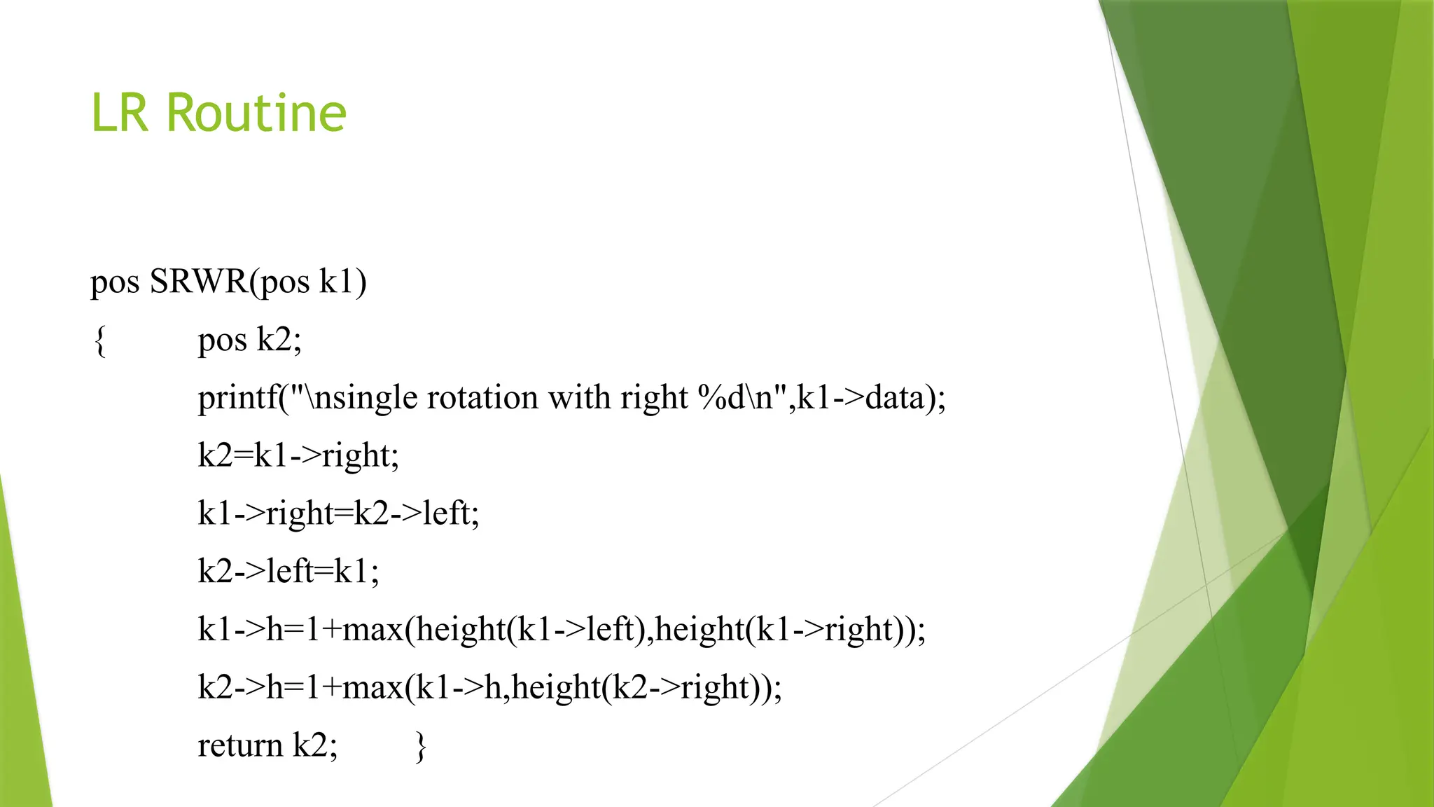
LR Routine pos SRWR(pos k1) { pos k2; printf("nsingle rotation with right %dn",k1->data); k2=k1->right; k1->right=k2->left; k2->left=k1; k1->h=1+max(height(k1->left),height(k1->right)); k2->h=1+max(k1->h,height(k2->right)); return k2; }

Double Rotation With Left(Left-Right Rotation)  Imbalance occur when inserting data at Right of Lest sub tree,

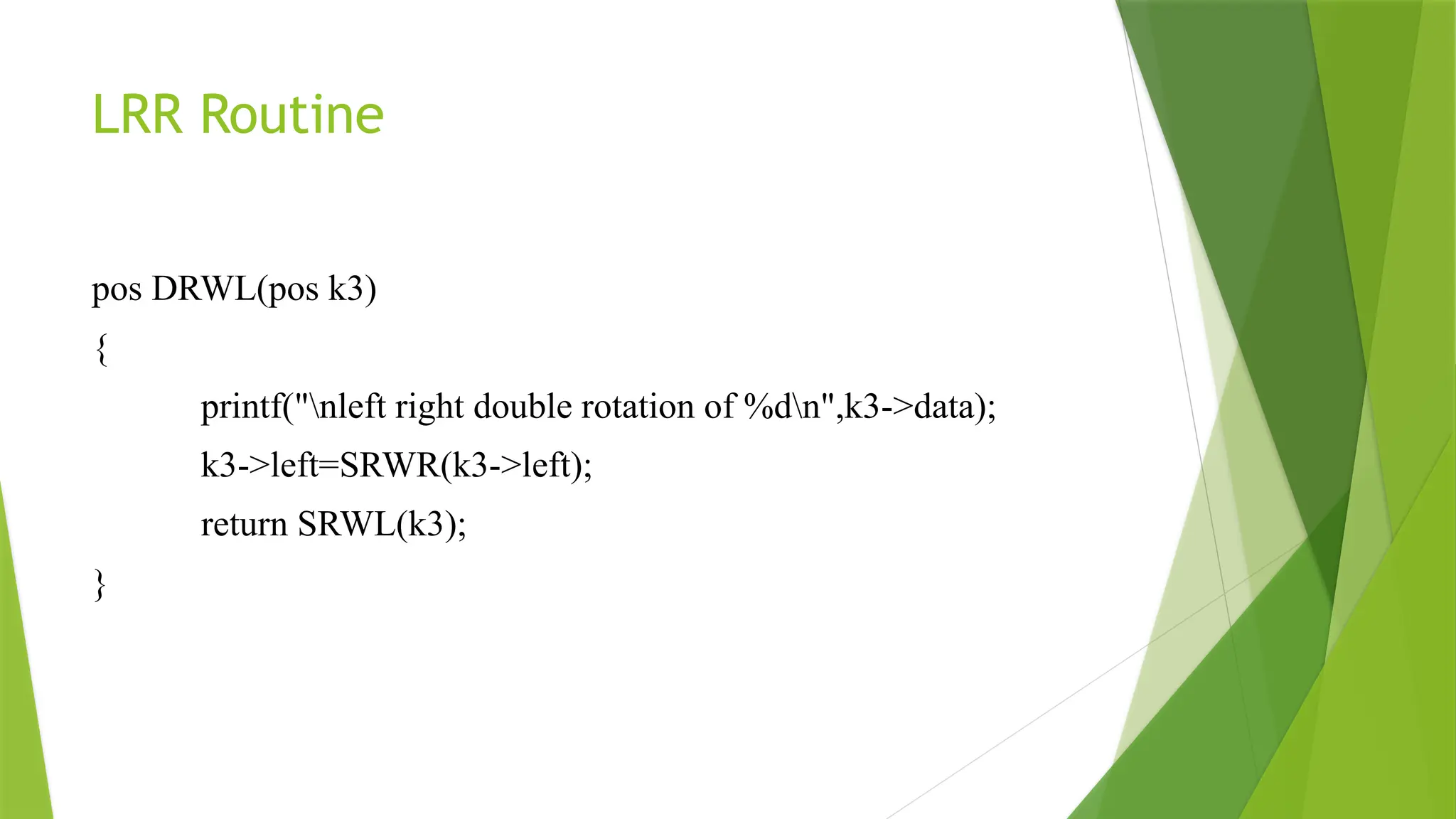
LRR Routine pos DRWL(pos k3) { printf("nleft right double rotation of %dn",k3->data); k3->left=SRWR(k3->left); return SRWL(k3); }

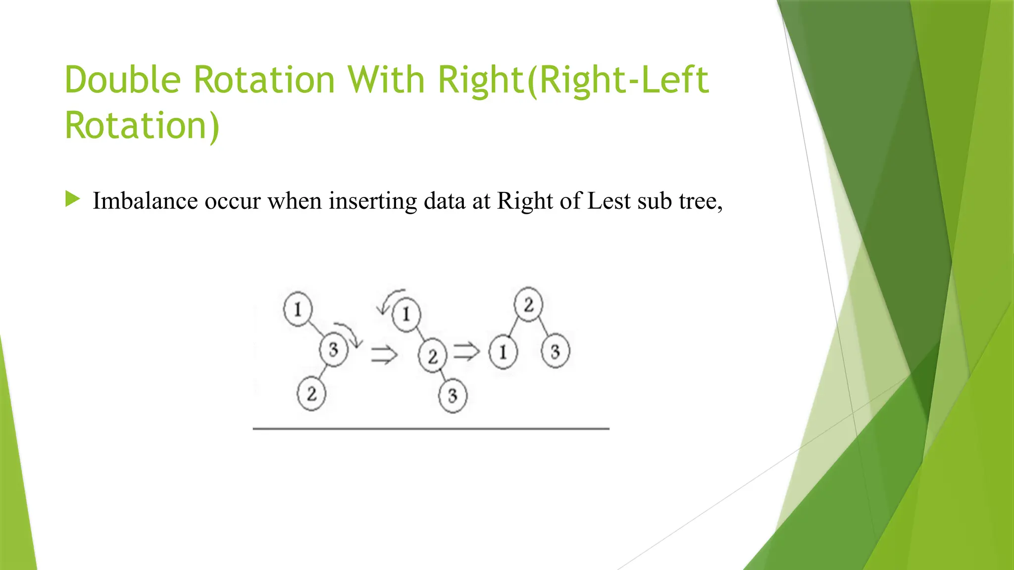
Double Rotation With Right(Right-Left Rotation)  Imbalance occur when inserting data at Right of Lest sub tree,

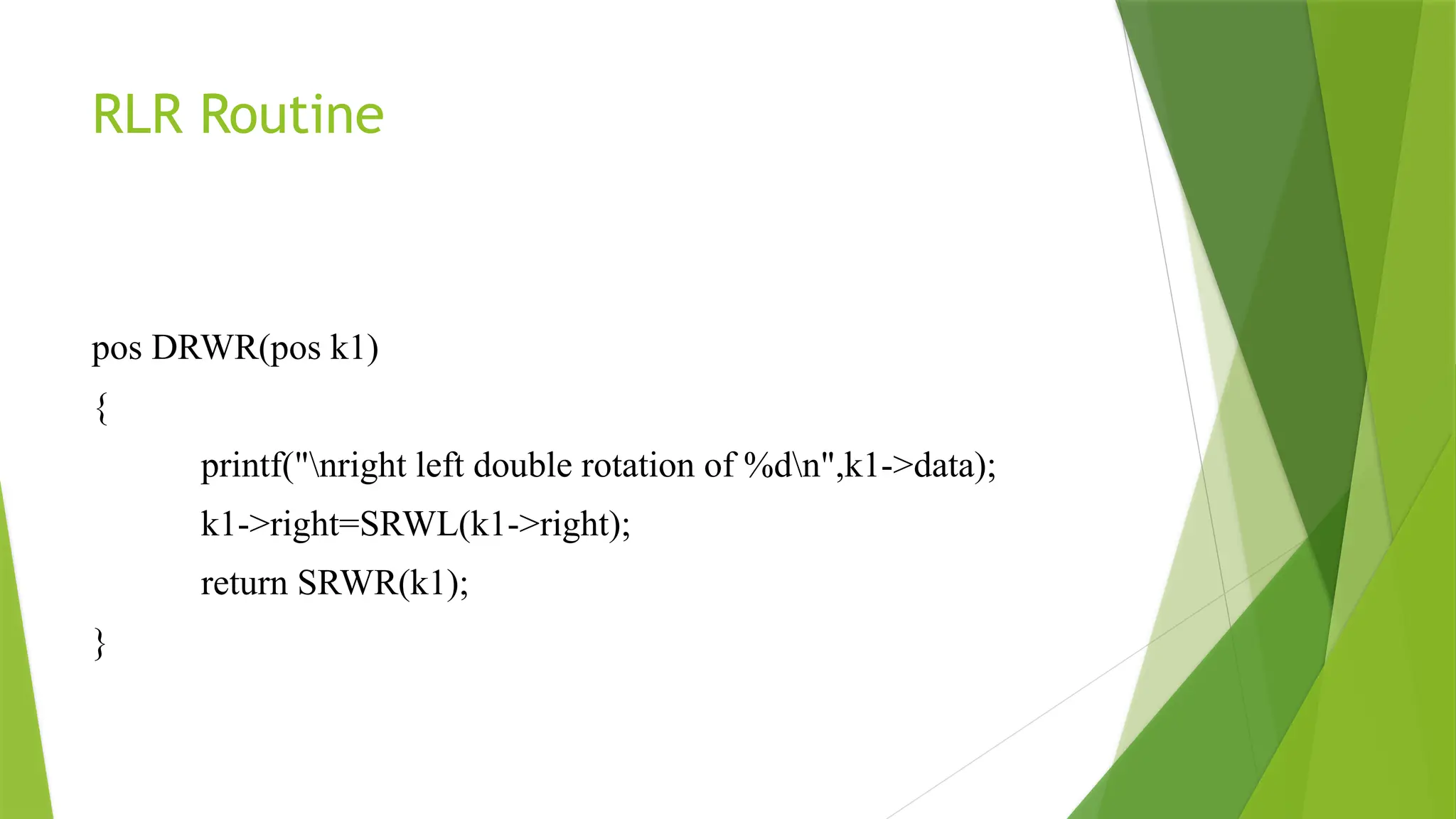
RLR Routine pos DRWR(pos k1) { printf("nright left double rotation of %dn",k1->data); k1->right=SRWL(k1->right); return SRWR(k1); }

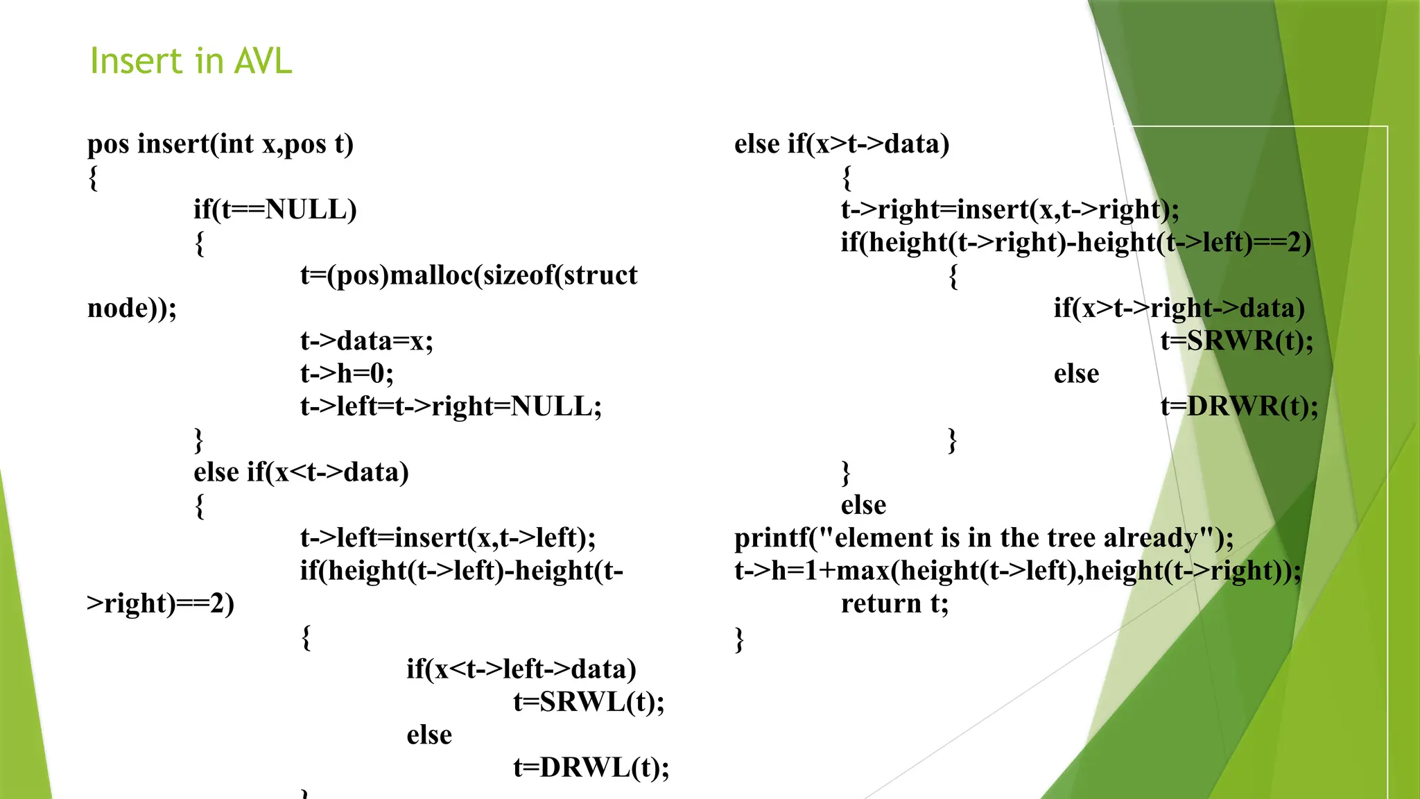
Insert in AVL pos insert(int x,pos t) { if(t==NULL) { t=(pos)malloc(sizeof(struct node)); t->data=x; t->h=0; t->left=t->right=NULL; } else if(x<t->data) { t->left=insert(x,t->left); if(height(t->left)-height(t- >right)==2) { if(x<t->left->data) t=SRWL(t); else t=DRWL(t); else if(x>t->data) { t->right=insert(x,t->right); if(height(t->right)-height(t->left)==2) { if(x>t->right->data) t=SRWR(t); else t=DRWR(t); } } else printf("element is in the tree already"); t->h=1+max(height(t->left),height(t->right)); return t; }

Two types of memory • Main memory (RAM) • External (peripheral) storage: hard disk, CD-ROM, tape, etc. Different considerations are important in designing algorithms and data structures for primary (main) versus secondary (peripheral) memory.

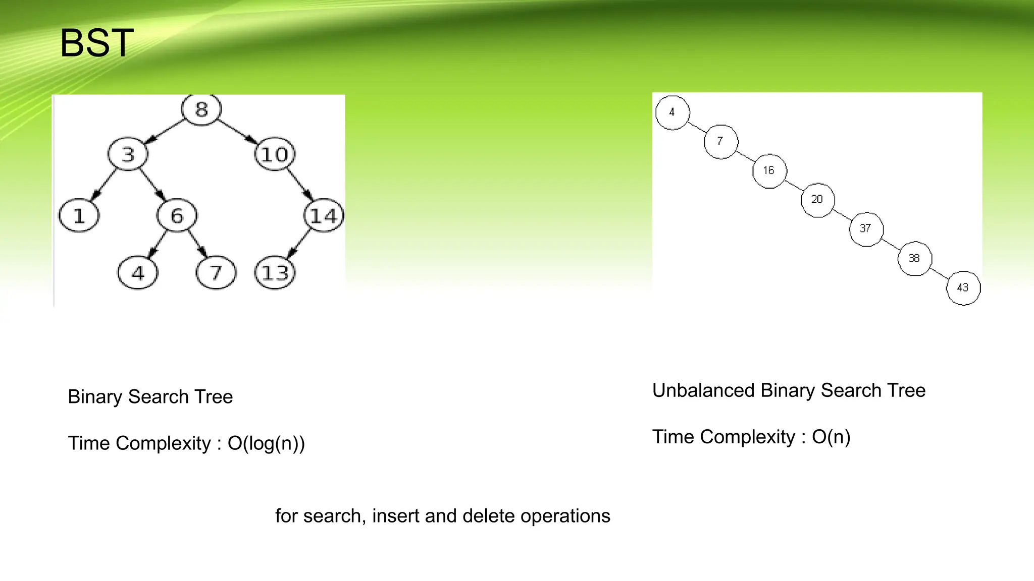
BST Binary Search Tree Time Complexity : O(log(n)) Unbalanced Binary Search Tree Time Complexity : O(n) for search, insert and delete operations

What is the remedy?? • Remedy is self balancing trees.  Automatically adjust to itself to get balanced.  eg Red black tree  B-Tree

What is B tree ? • Intro  Invented by Rudolf Bayer and Ed McCreight in 1972 at Boeing Research Labs.  B-Tree is known as balanced m-way tree and used in external sorting.  m-way node is were m=5 it describes that there should be m links and m-1 data.  Algorithms and data structures for external memory as opposed to the main memory

B Tree • A good example of a data structure for external memory is a B-tree. • Better than binary search trees if data is stored in external memory (they are NOT better with in-memory data!). • Each node in a tree should correspond to a block of data. • Each node stores many data items and has many successors (stores addresses of successor blocks).

• The tree has fewer levels but search for an item involves more comparisons at each level. • There is a single root node, which may have only one record and two children (or none if the tree is empty).

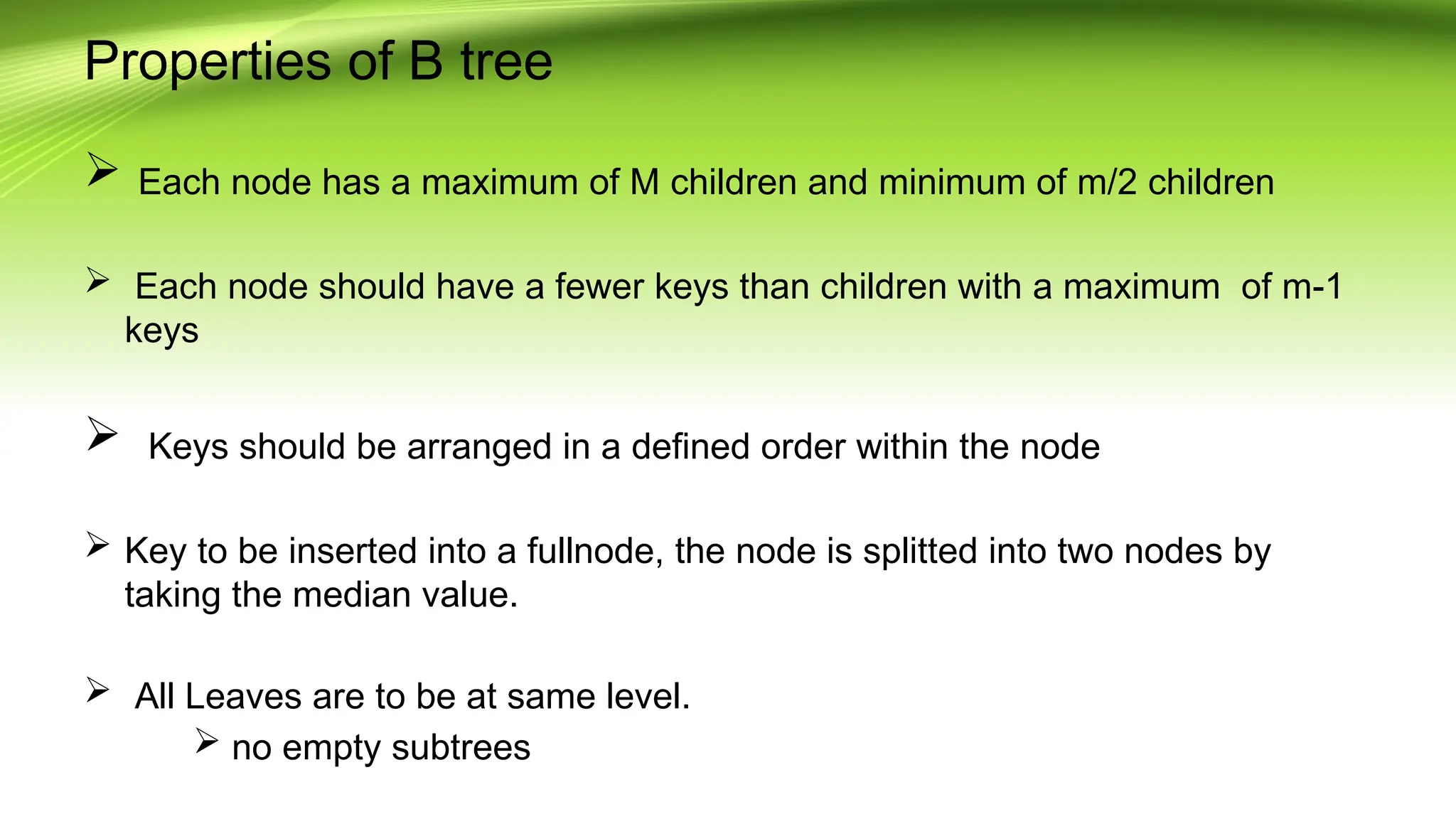
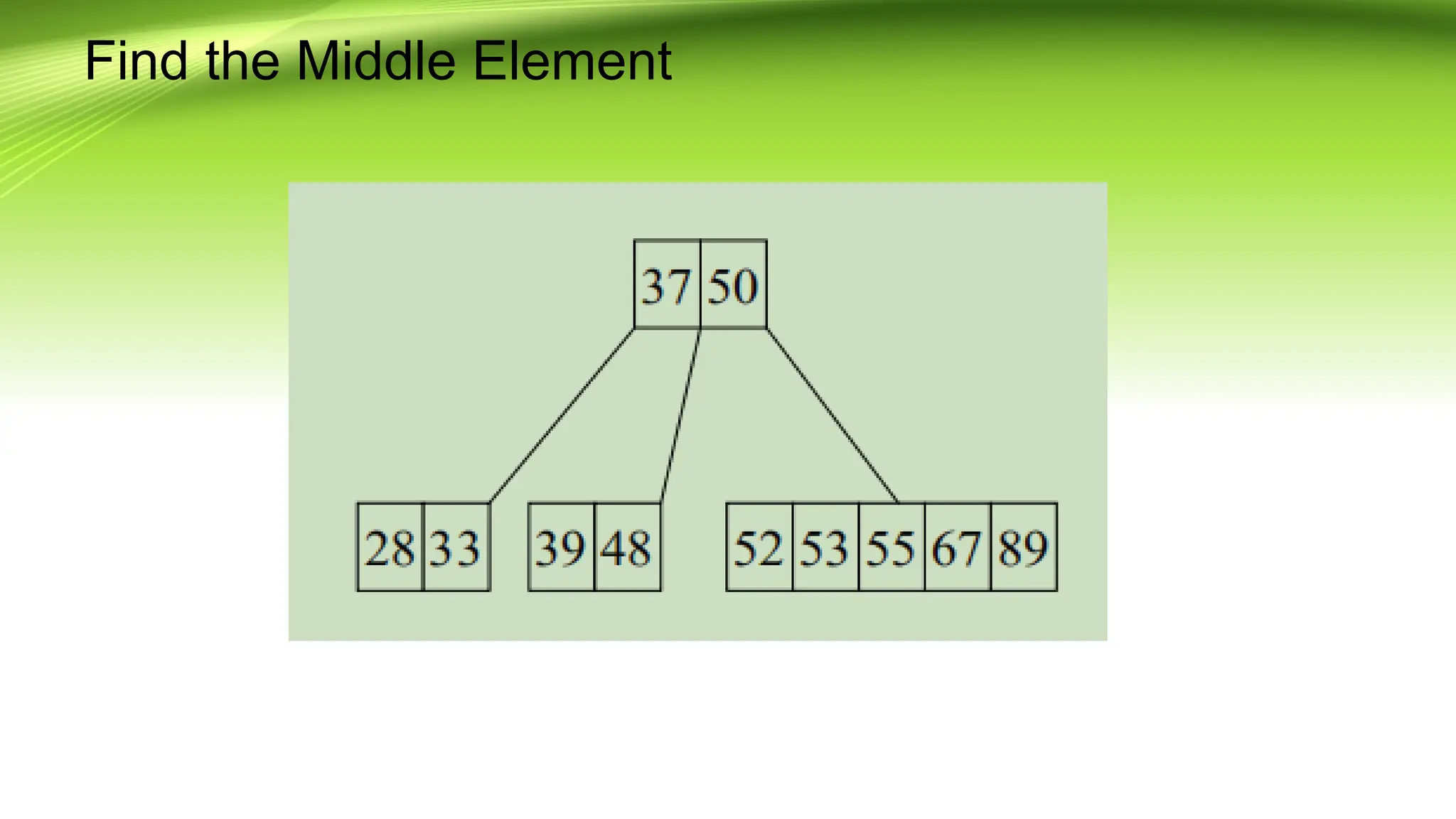
Properties of B tree  Each node has a maximum of M children and minimum of m/2 children  Each node should have a fewer keys than children with a maximum of m-1 keys  Keys should be arranged in a defined order within the node  Key to be inserted into a fullnode, the node is splitted into two nodes by taking the median value.  All Leaves are to be at same level.  no empty subtrees

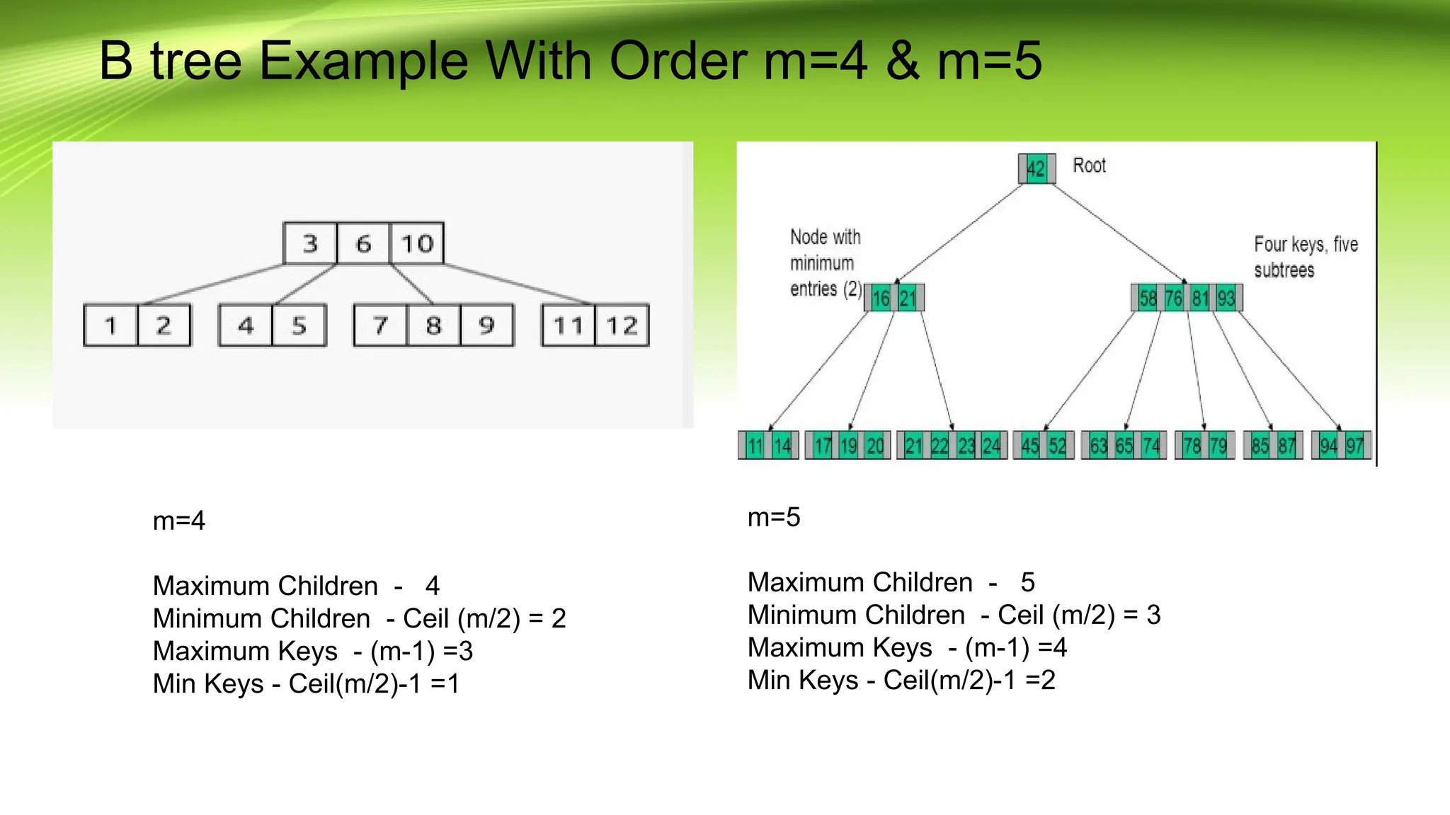
B tree Example With Order m=4 & m=5 m=4 Maximum Children - 4 Minimum Children - Ceil (m/2) = 2 Maximum Keys - (m-1) =3 Min Keys - Ceil(m/2)-1 =1 m=5 Maximum Children - 5 Minimum Children - Ceil (m/2) = 3 Maximum Keys - (m-1) =4 Min Keys - Ceil(m/2)-1 =2

Operations on B trees • Basic three opeartions  Insertion  Insertion will be done in the leaf nodes  Deletion  Search

Search for record with key 40:

Inserting 53: the node is too full!

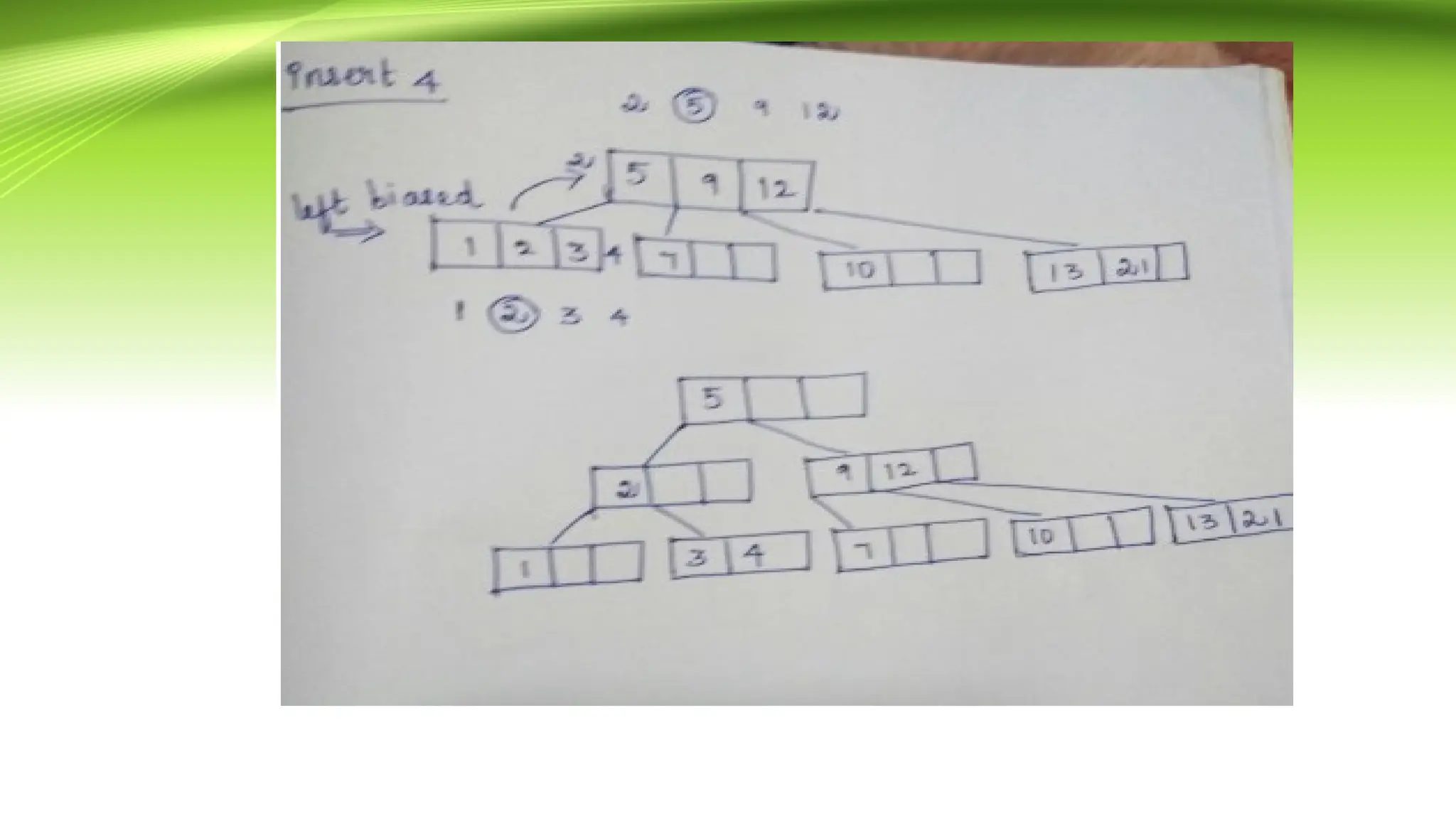
Insertion with even order • To insert elements in B tree element to be inserted is to be scanned from left to right.  If the order to construct an even order B tree then two sets of tree is created • Left Biased • Right Biased

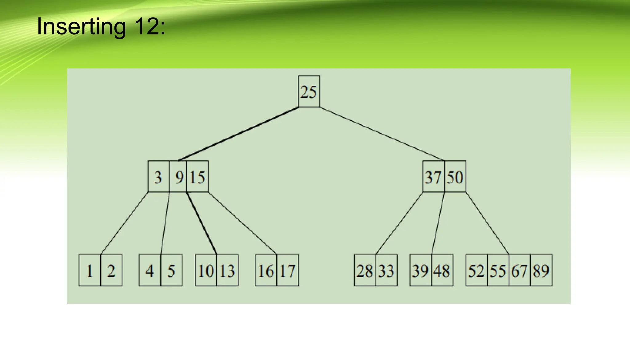
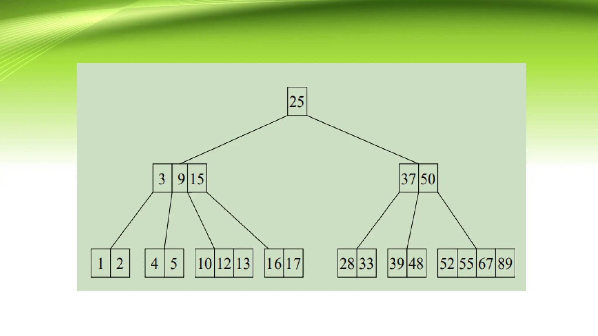
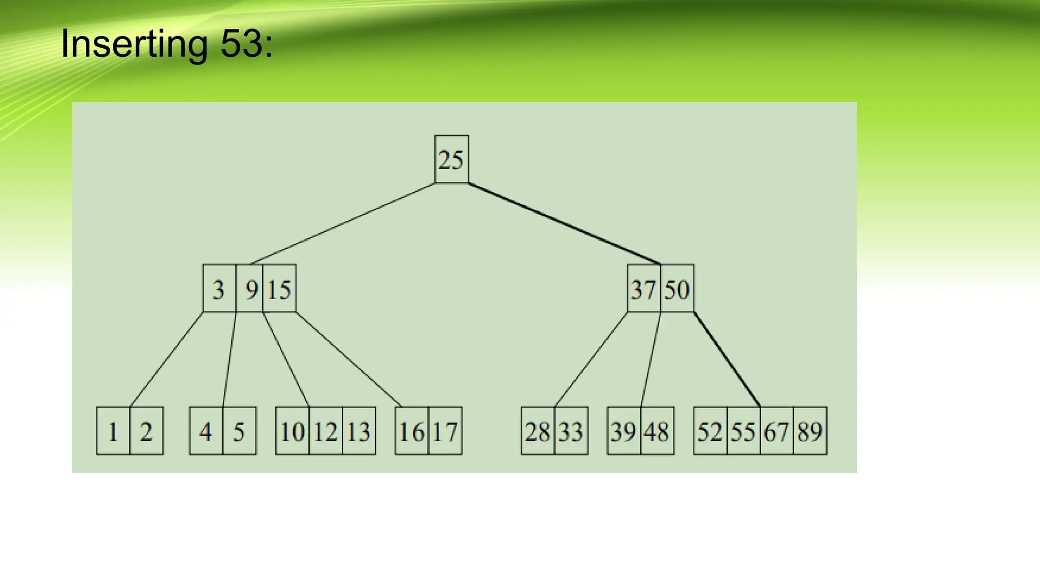
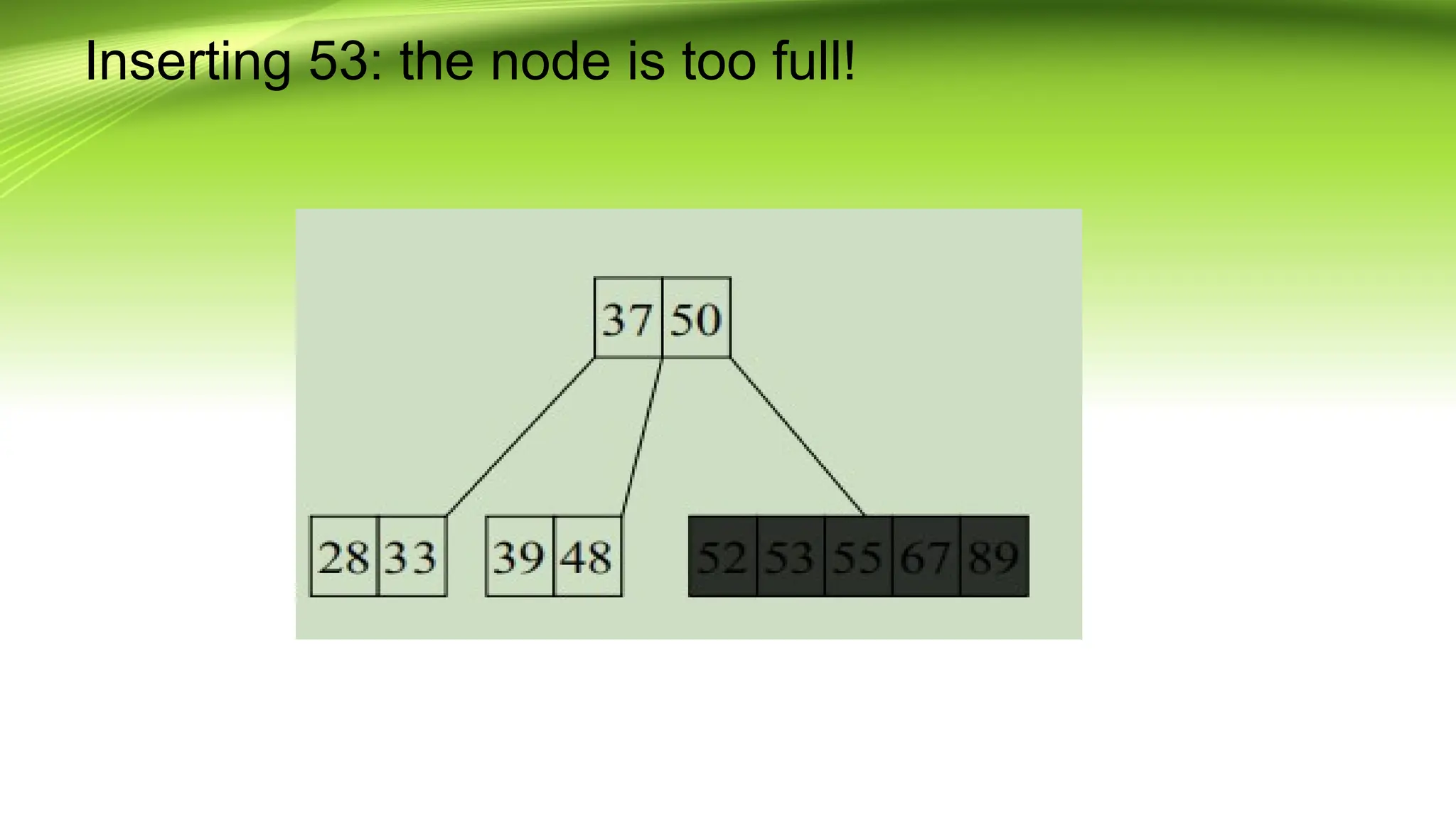
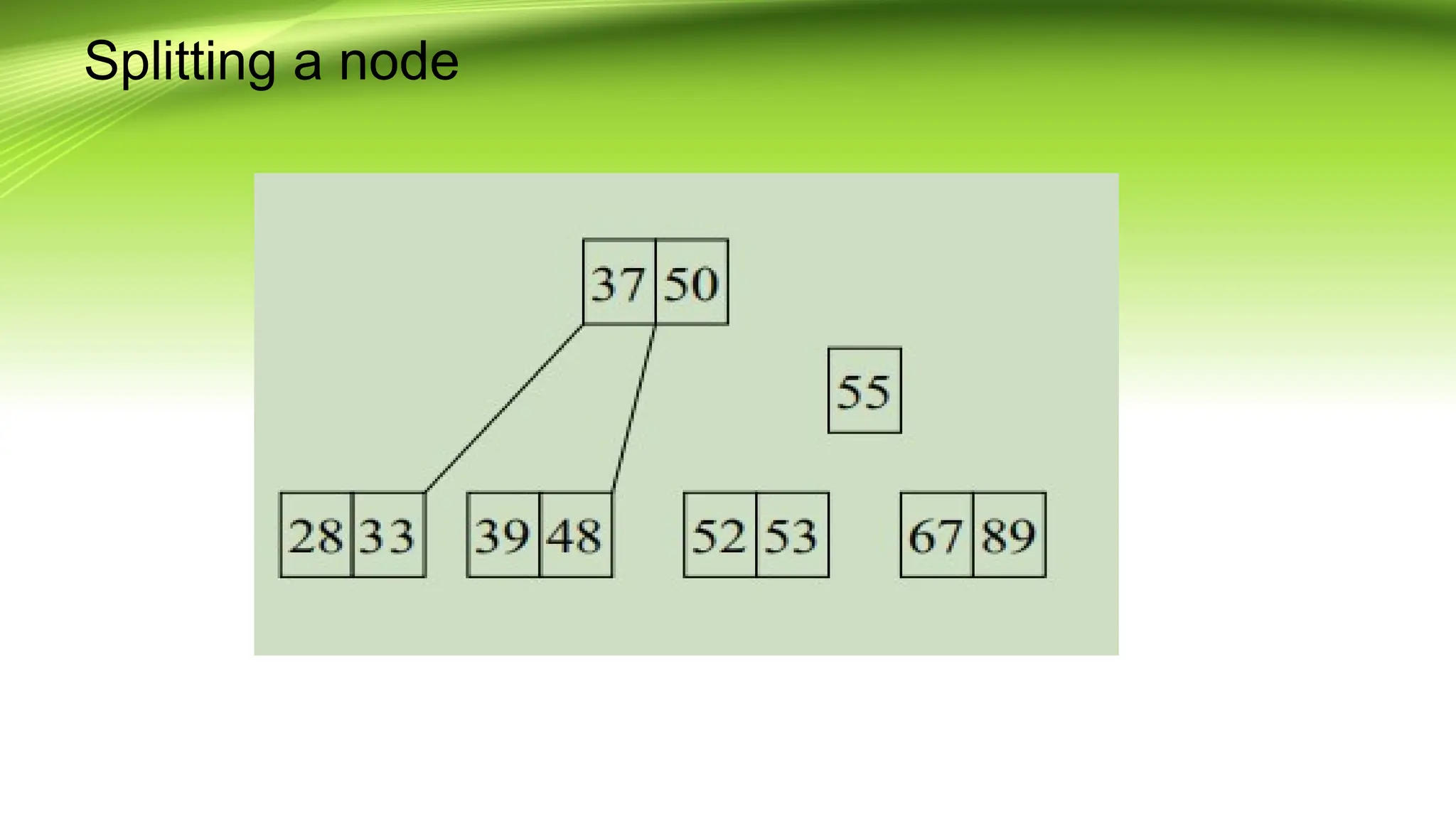
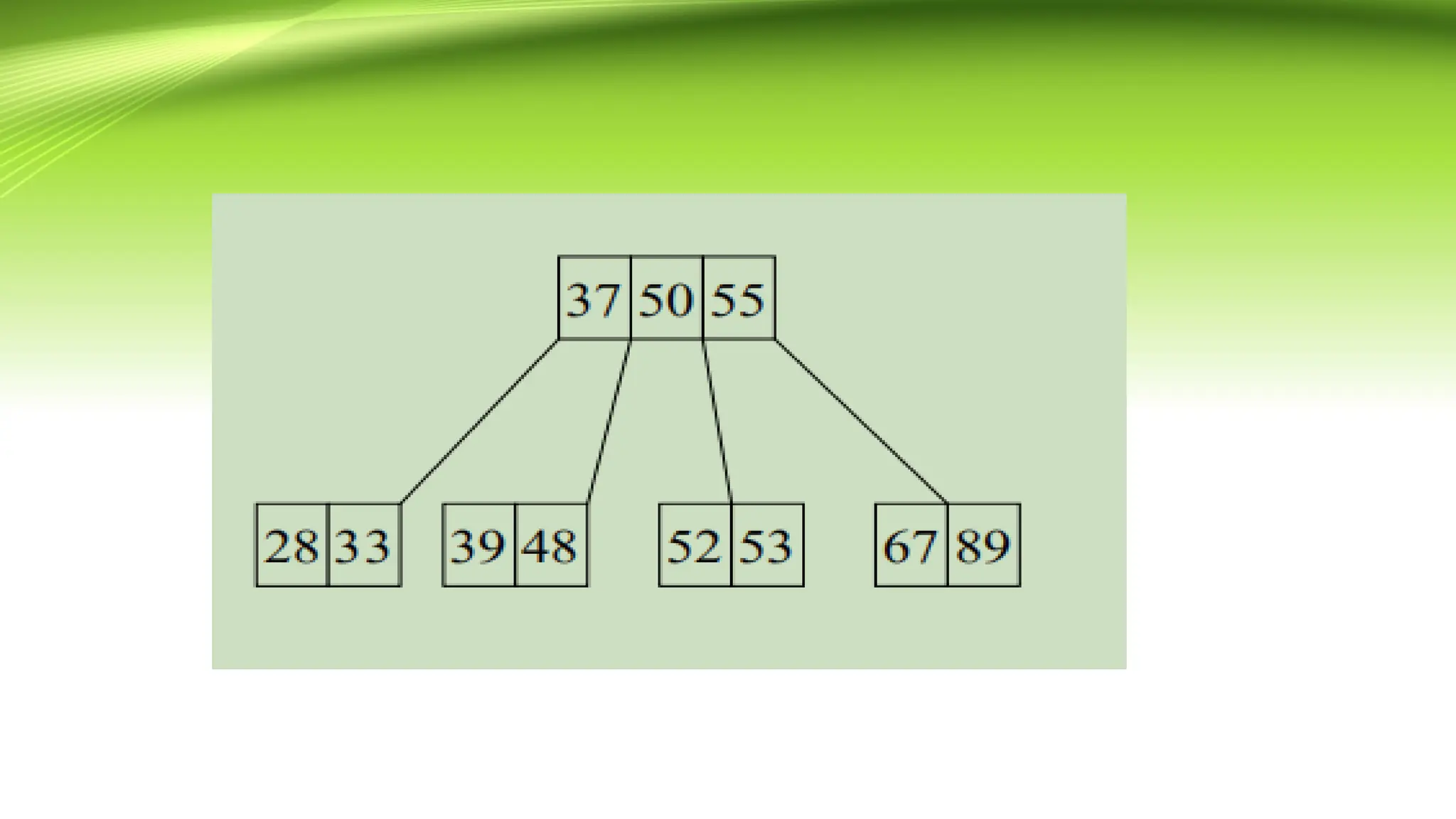
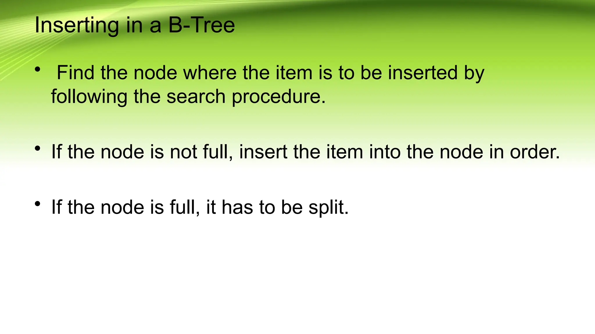
Inserting in a B-Tree • Find the node where the item is to be inserted by following the search procedure. • If the node is not full, insert the item into the node in order. • If the node is full, it has to be split.

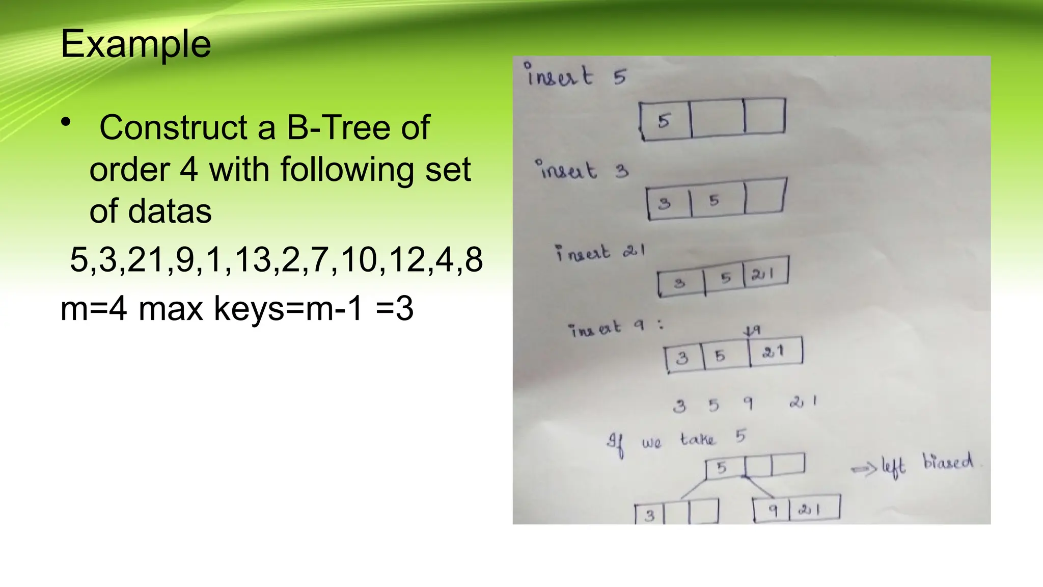
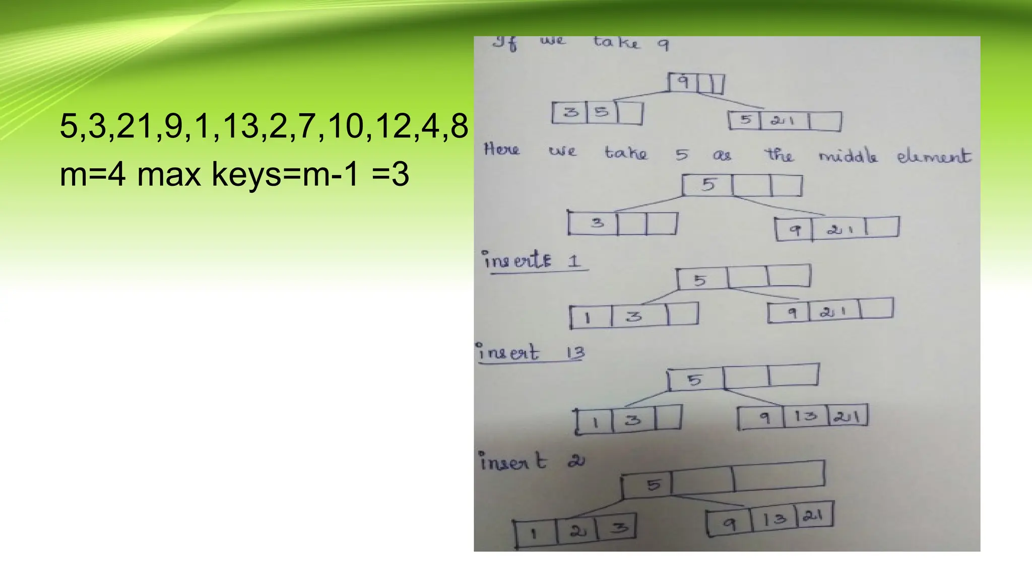
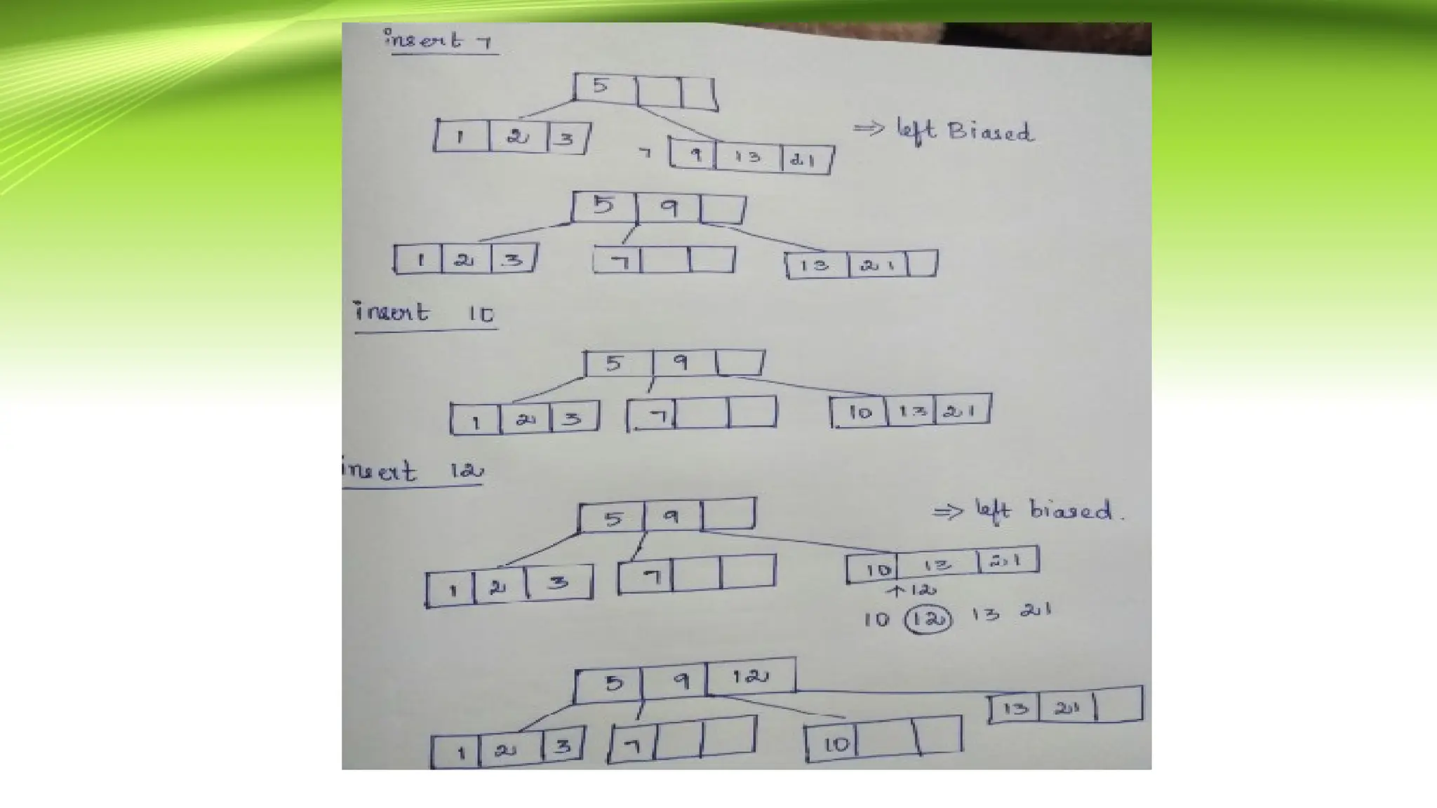
Example • Construct a B-Tree of order 4 with following set of datas 5,3,21,9,1,13,2,7,10,12,4,8 m=4 max keys=m-1 =3

5,3,21,9,1,13,2,7,10,12,4,8 m=4 max keys=m-1 =3

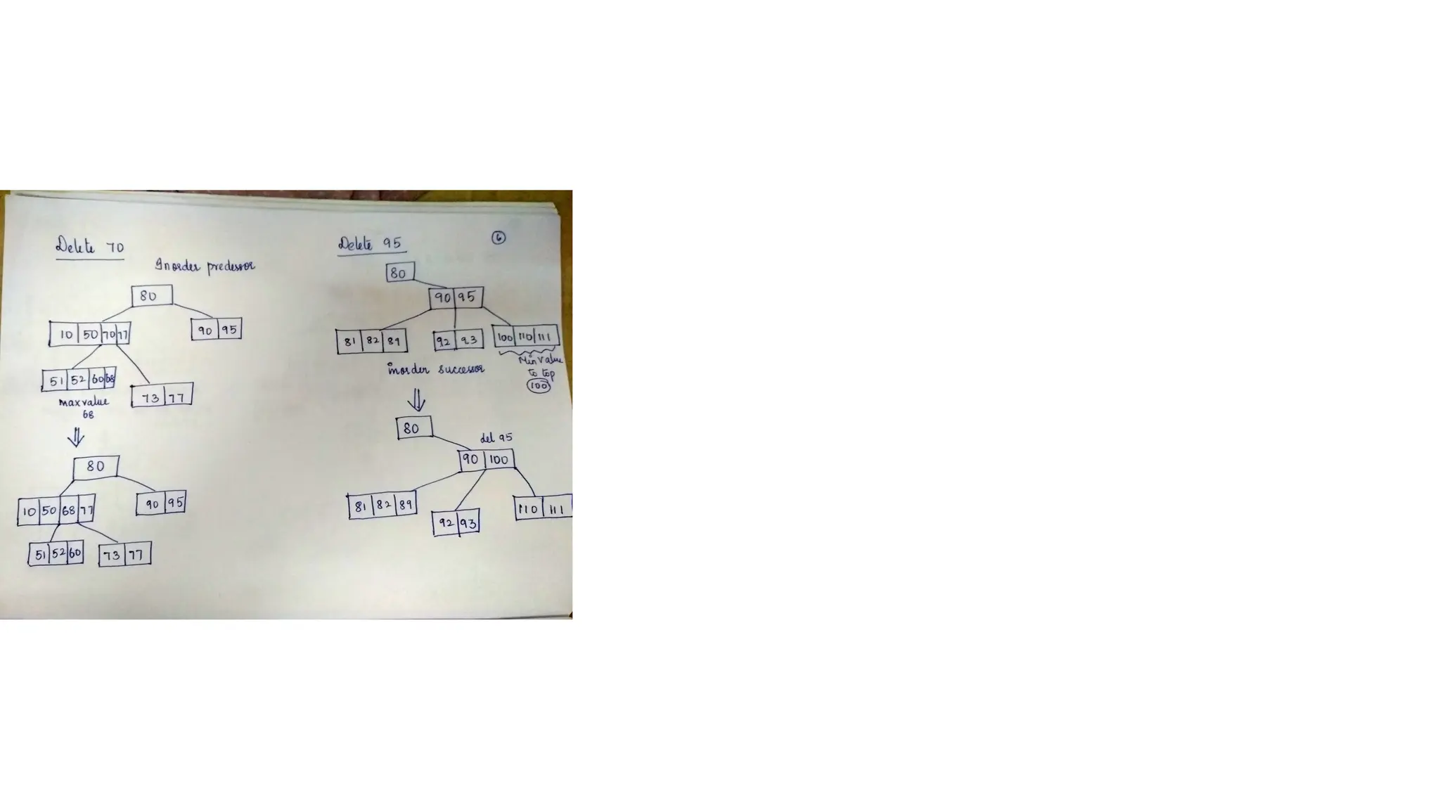
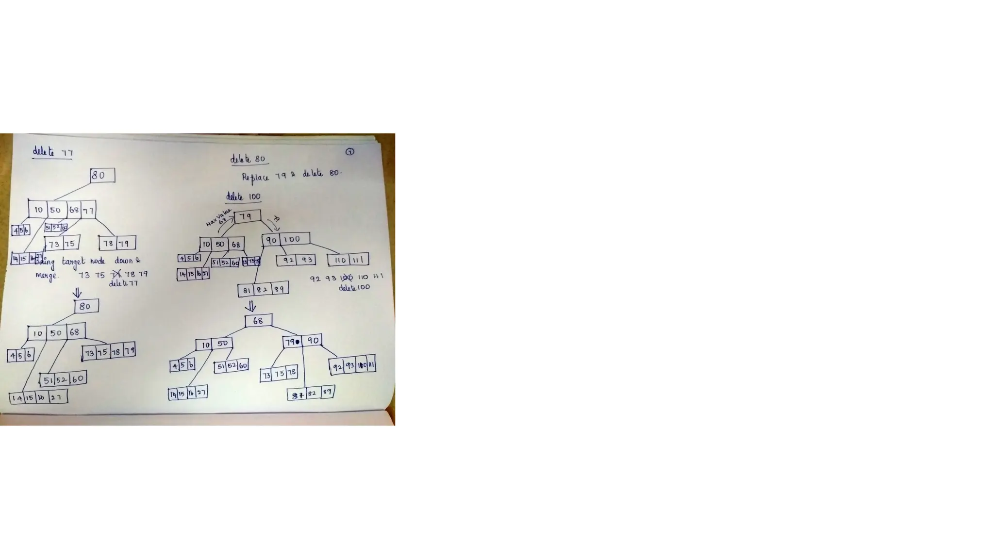
Deletion in B tree • The key to be deleted is called the target key Two Possibilities  Target key can be a leaf node  Target Key can be in internal node

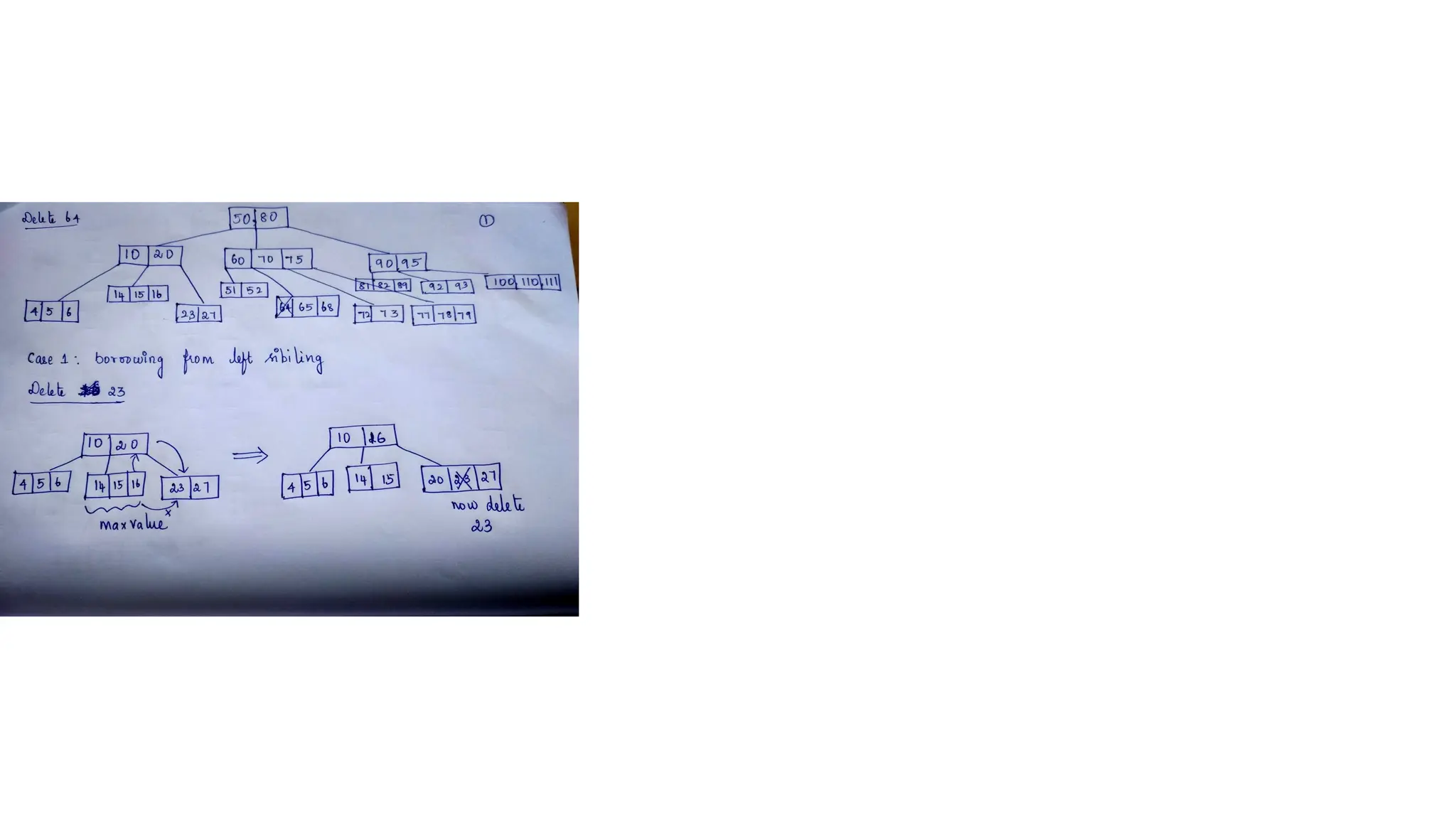
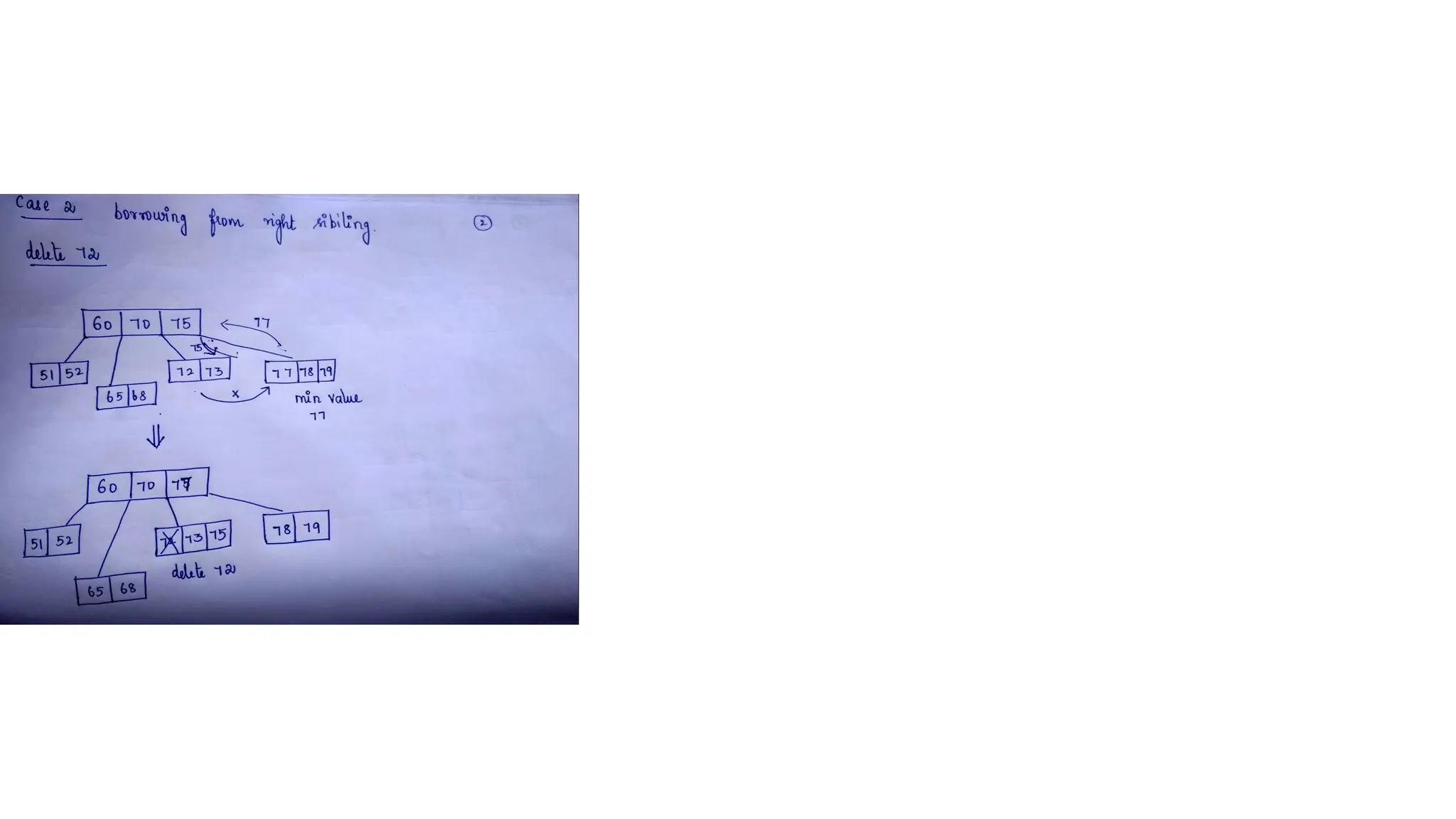
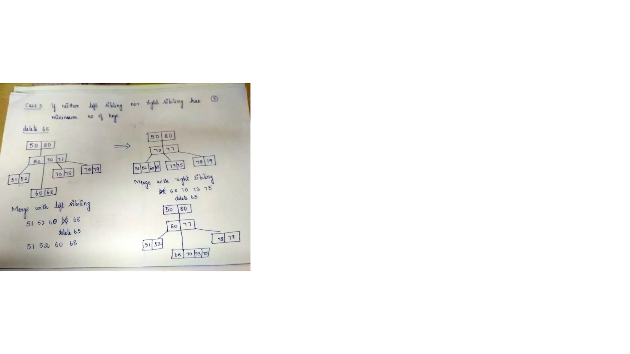
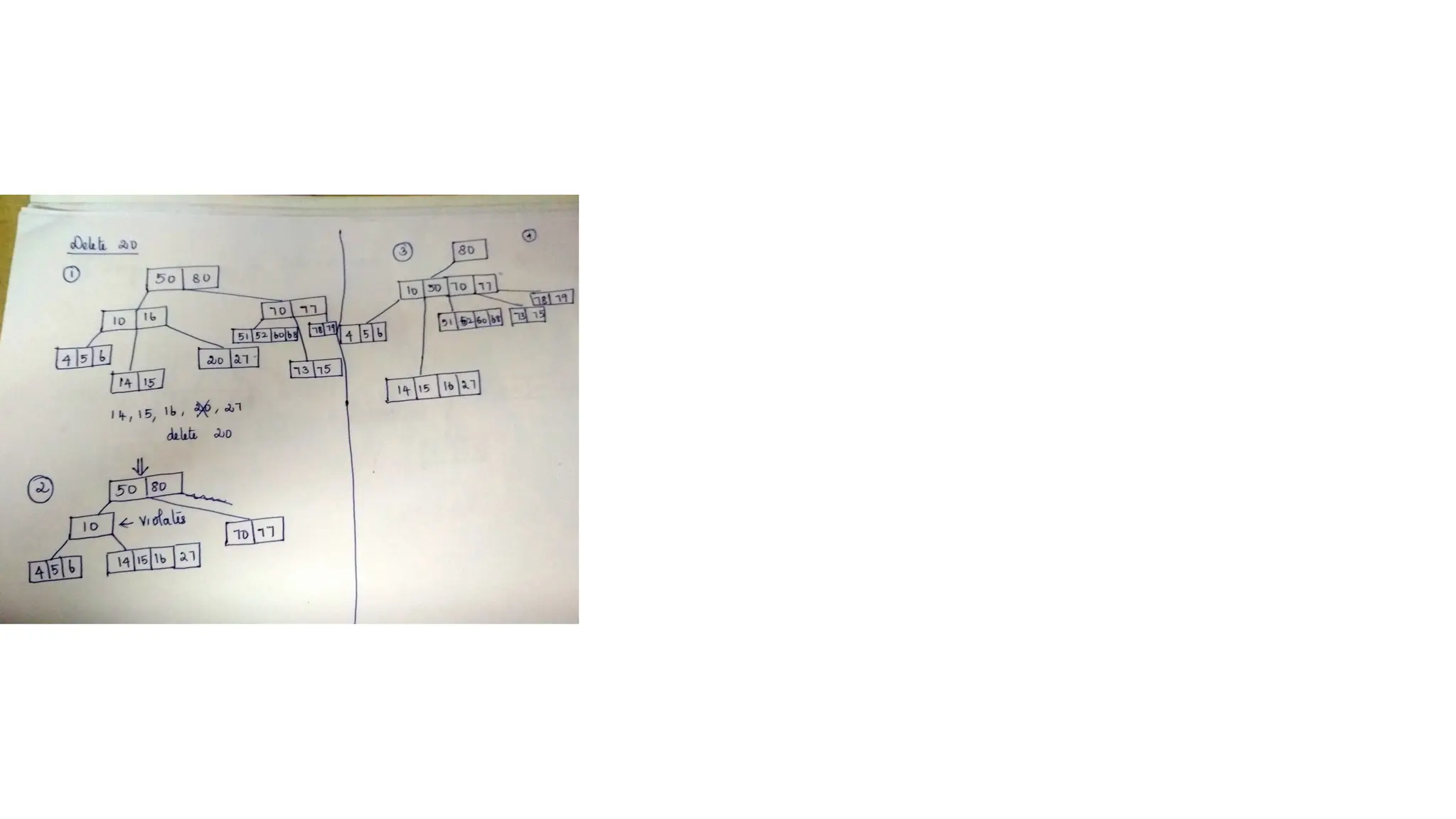
Contd.. • Target key can be leaf node Two Possibilities  Leaf node contains more than min no of keys  Leaf node contains min no of keys  borrow from immediate left node  borrow from immediate right node  borrow from root and merge

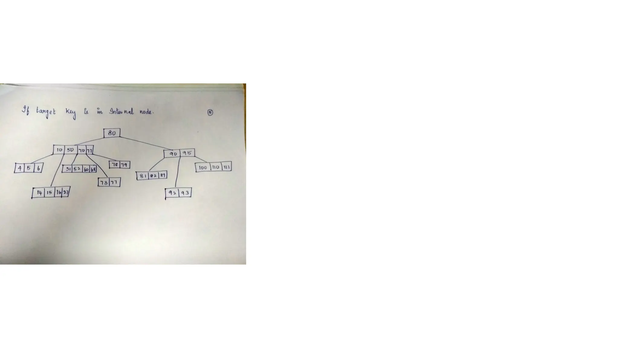
Contd.. • If the target key is internal node  perform inorder predecessor  perform inorder successor  Merge with root

Tree Data Structures with Types, Properties, Traversals, Advanced Variants, and Applications in Computer Science

More Related Content

Similar to Tree Data Structures with Types, Properties, Traversals, Advanced Variants, and Applications in Computer Science

More from usham61

Recently uploaded

Tree Data Structures with Types, Properties, Traversals, Advanced Variants, and Applications in Computer Science