Transient Stability Enhancement of a Multi-Machine System using Particle Swarm Optimization based Unified Power Flow Controller

Transient Stability Enhancement of a Multi-Machine System using Particle Swarm Optimization based Unified Power Flow Controller

• 1.
  Poonam Singhal etal Int. Journal of Engineering Research and Applications www.ijera.com ISSN : 2248-9622, Vol. 4, Issue 7( Version 3), July 2014, pp.121-133 www.ijera.com 121|P a g e Transient Stability Enhancement of a Multi-Machine System using Particle Swarm Optimization based Unified Power Flow Controller Poonam Singhal1, S. K. Agarwal2, Narender Kumar3 Abstract In this paper an attempt has beenmade to investigate the transient stability enhancement of both SMIB and Multi-machine system using UPFC controller tuned by Particle Swarm Optimization. Power injection modelfor a series voltage source of UPFC has been implemented to replace UPFC by equivalent admittance. The admittance matrix of the power system is then modified according to the power injection model of UPFC. To mitigate the power oscillations in the system, the required amount of series voltage injected by UPFC controller has been computed in order to damp inter area & local mode of oscillations in multi-machine system. Keywords:UPFC, Transient Stability, Converters, SMIB, Multi-machine modeling, Capacitor Dynamics,UPFC(Unified Power Flow Controller), FACTS (Flexible AC Transmission System), Power injection model. Particle Swarm Optimization. I. INTRODUCTION Modern interconnected power system comprise a number of generators, a large electrical power network & a variety of loads& such a complex system is vulnerable to sudden faults, load changes & uncertain nature resulting in instability & so the designing of such a large interconnected power systems to ensure secure & stable operation is a complicated problem. The power transmission network is an important element of the power system which is responsible for causing instability, sudden voltage collapse during transient conditions. In recent years, technologically developments in Flexible AC Transmission Systems or FACTS devices [1] provided better performance in enhancing power system. The FACTS envisage the use of a solid state power converter technology to achieve fast & reliable control of power flow in transmission line. The greatest advantage of using a FACTS device in a power transmission network is to enhance the transient stability performance by controlling the real & reactive power flow during fault conditions. The FACTS devices are classified into two categories; the shunt type comprises of SVC [21]&STATCOM while the series comprises of TCSC & TCPST. UPFC is the most versatile belong to FACTS family which combines both shunt & series features. It is capable of instantaneous control of transmission line parameters [5].The UPFC can provide simultaneous control of all or selectively basic parameters of power system [6, 7, 20] (transmission voltage, line impedance and phase angle) and dynamic compensation of AC power system. In this paper UPFC is used to inject thevariable voltage in series with the line, whose magnitude can varies from 0 to Maximumvalue (depends on rating) and phase angle can differ from 0 to 2π which modulates the line reactance to control power flow in transmission line. By regulating the power flow in a transmission line, the speed of oscillations of the generator can be damped effectively. II. UPFC DESCRIPTION The UPFC constitute of two voltage source converters linked with common DC link. One of the converters is connected in series (known as series converter or SSSC) with the line via injection transformer and provides the series voltage and other converter (called shunt converter or STATCOM) is connected in parallel via shunt transformer to inject the shunt current and also supply or absorb the real power demand by series converter at common dc link. The reactive power exchanged at the ac terminal of series transformer is generated internally by voltage source converter connected in series. The voltage source converter connected in shunt can also generate or absorb controllable reactive power, thus providing shunt compensation for the line independent of the reactive power exchange by the converter connected in series. The UPFC, thus, can be summarize as an ideal ac to ac power converter in which real power can flow freely in either direction between the ac terminal of the two converters and reactive power can be generated or absorbed by the two converters independently at their own ac terminals. Figure 1 shows the equivalent circuit of the UPFC in which the UPFC can be represented as a two port device with controllable voltage source Vse in series with line and controllable shunt current source Ish. The voltage across the dc capacitor is RESEARCH ARTICLE OPEN ACCESS
• 2.
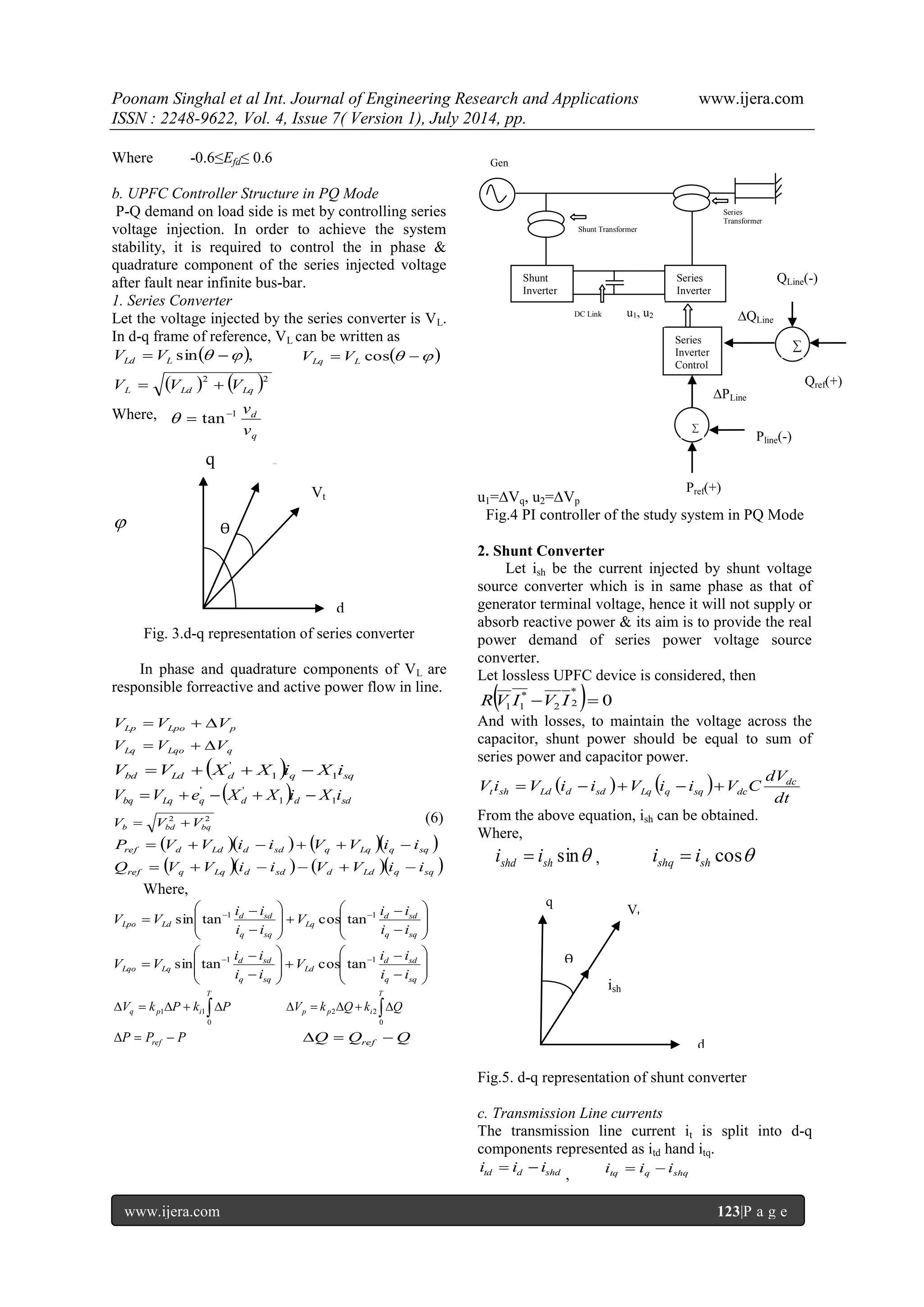
  Poonam Singhal etal Int. Journal of Engineering Research and Applications www.ijera.com ISSN : 2248-9622, Vol. 4, Issue 7( Version 1), July 2014, pp. www.ijera.com 122|P a g e maintained constant because the UPFC as a whole does not generate or absorb any real power. In this paper, the UPFC is used to damp the power oscillations and thus improves the transient stability of both SMIB and multi-machine power system.UPFC parameters have been optimized using Bacterial Foraging in paper [16]. Particle Swarm Optimization technique, another heuristic technique based on bird and fish flock movement behavior is implemented for optimizing the parameters of UPFC efficiently and effectively in real time. In this paper, section II describes about the UPFC. Section III explains the brief description of the SMIB test systemtaken whereas section IV explains the mathematical modeling of the SMIB system equipped with UPFC Controller. Section V briefly describes the multi-machine power system under study. Section VI illustrates the modeling ofmulti-machine power system. Modeling of unified power flow controller for load flow is illustrated in Section VII. Section VIII illustrates the simulation results ofboth SMIB system and multi-machine system without and with UPFC controller based on PSO and section IX concludes and expresses the future scope of work. Fig. 1.Equivalent Circuit of UPFC III. SMIB SYSTEM UNDER STUDY For analysis of the UPFC for damping the power swings, parameters of the system like generator rotor angle, theta, terminal voltage, active power and reactive power are considered. A 200MVA, 13.8KV, 50Hz generator supplying power to an infinite bus through two transmission circuits as shown in fig(2) is considered. The network reactance shown in fig. is in p.u. at 100 MVA base. Resistances are assumed to be negligible. The system is analyzed with different initial operating condition, with quantities expressed in p.u. on 100MVA, 13.8 KV base. P=0.4p.u, 0.8p.u, 1.2p.u and 1.4p.u are different operating conditions considered. The other generator parameters in p.u. are given in appendix. The three phase fault at infinite bus bar is created for 100msec duration & simulation is carried out for 10sec. to examine the transient stability of the study system. Fig 2. IV. MATHEMATICAL MODELING a. Synchronous Machine Model Mathematical models of synchronous machine vary from elementary classical model to more detailed one. Here, the synchronous generator is represented by third order machine model [2,4]. Different equations for stator, rotor, excitation system etc. are as follows: Stator: q q s q d d V E r i x i ' '    d d s d q q V E r i x i ' '    d q V  v  jv 1 d q I  i  ji * 1S  V I d d q q P  v i  v i q d d q Q  v i  v i Where, dt d     M P P dt m e    Let D and K=0 s r is rotor winding resistance ' d x is d-axis transient reactance ' q x is q-axis transient reactance ' d E is d-axis transient voltage ' q E is q-axis transient voltage Rotor:   q f d d d q do E E x x i dt dE T ' ' ' '       ' ' ' ' do q f q d d d T E E x x i dt dE     Where, ' do T is d-axis open-circuit transient time constant ' qo T is q-axis open-circuit transient time constant f E is field voltage Torque Equation   e q q d d q d d q T E i E i x x i i ' ' ' '     Excitation System Te fd E Te Vt ref Ke V dt fd d E     ( ) ( ) V 1 V2 I1 I2 Ish Vse Gen Bus1 Bus2 UPFC
• 3.
  Poonam Singhal etal Int. Journal of Engineering Research and Applications www.ijera.com ISSN : 2248-9622, Vol. 4, Issue 7( Version 1), July 2014, pp. www.ijera.com 123|P a g e Where -0.6≤Efd≤ 0.6 b. UPFC Controller Structure in PQ Mode P-Q demand on load side is met by controlling series voltage injection. In order to achieve the system stability, it is required to control the in phase & quadrature component of the series injected voltage after fault near infinite bus-bar. 1. Series Converter Let the voltage injected by the series converter is VL. In d-q frame of reference, VL can be written as  sin  , Ld L V V  cos   Lq L V V    2 2 L Ld Lq V  V  V Where, q d v v 1 tan    Fig. 3.d-q representation of series converter In phase and quadrature components of VL are responsible forreactive and active power flow in line. Lp Lpo p V V  V Lq Lqo q V V  V   bd Ld d q sq V V X X i X i 1 1 '       bq Lq q d d sd V V e X X i X i 1 1 ' '      2 2 b bd bq V  V V (6)       ref d Ld d sd q Lq q sq P  V V i  i  V V i  i       ref q Lq d sd d Ld q sq Q  V V i  i  V V i  i Where,                         q sq d sd Lq q sq d sd Lpo Ld i i i i V i i i i V V 1 1 sin tan cos tan                         q sq d sd Ld q sq d sd Lqo Lq i i i i V i i i i V V 1 1 sin tan cos tan       T q p i V k P k P 0 1 1      T p p i V k Q k Q 0 2 2 P P P ref    Q Q Q ref    u1=ΔVq, u2=ΔVp Fig.4 PI controller of the study system in PQ Mode 2. Shunt Converter Let ish be the current injected by shunt voltage source converter which is in same phase as that of generator terminal voltage, hence it will not supply or absorb reactive power & its aim is to provide the real power demand of series power voltage source converter. Let lossless UPFC device is considered, then   0 * 2 2 * 1 1 RV I V I  And with losses, to maintain the voltage across the capacitor, shunt power should be equal to sum of series power and capacitor power.     dt dV V i V i i V i i V C dc t sh Ld d sd Lq q sq dc      From the above equation, ish can be obtained. Where, sin shd sh i  i , cos shq sh i  i Fig.5. d-q representation of shunt converter c. Transmission Line currents The transmission line current it is split into d-q components represented as itd hand itq. td d shd i  i  i , tq q shq i  i i q Vt d Ө    q Vt d Ө ish Gen Shunt Transformer Series Transformer DC Link Shunt Inverter Series Inverter Series Inverter Control u1, u2 ΔQLine Σ Σ QLine(-) Qref(+) ΔPLine Pline(-) Pref(+)
• 4.
  Poonam Singhal etal Int. Journal of Engineering Research and Applications www.ijera.com ISSN : 2248-9622, Vol. 4, Issue 7( Version 1), July 2014, pp. www.ijera.com 124|P a g e d. Capacitor Dynamics The difference between the shunt power and series power is the capacitor power. Mathematically, Capacitor power=Shunt power– Series power dc sh se dc V P P dt dV C       sh t sh P V i se Ld td Lq tq P V i V i   dc t sh Lp td Lq tq dc V V i V i V t dt dV C        ish then can be computed from the above equation V. DESCRIPTION OF MULTI-MACHINE SYSTEM A multi-machine power system (8 bus system) with twoUPFC‟s connected are considered as shown in fig 2. Three generators are connected at buses 1, 2 and 3.Generator 1 is hydro & G2 & G3 are Thermalgenerators.The parameters of all the generators are given in appendix. Bus number 1 is taken as slack bus. The transmission line parameters are also given in appendix.UPFC1 is connected between bus number 4 and 5, while UPFC2 is connected between bus number 7 and 8. Loads are connected at bus number 1, 2 and 3. They are represented in terms of admittances YL1, YL2, YL3 and YL4& are computed from load bus data. Using power Injection model[19] of UPFC1 and UPFC2, they are represented by equivalent admittances and the admittance matrix of the power network is then modified. Simple AVR are connected to each generator. The operating conditions taken are: p1=4.5, q1=1.5, p2=1.3, q2=0.6,p3= 1.0,q3=0.5. Fault is created at the Centre of line3-4at 0.5 sec & cleared at 0.6 sec which results in power deviation in the transmission line. The real power deviation in the transmission line generates the component VSEQ of series voltage injection in quadrature with line current and the reactive power deviation in line generates the in phase component VSEP. kp and ki relates these components to power deviations. These PI controller parameters are then tuned by PSO technique to damp the inter area and local area oscillations effectively. VI. MATHEMATICAL MODELING A. Synchronous Machine Model Mathematical models of synchronous machine vary from elementary classical model to more detailed one. Fig. 6 Here, the synchronous generator is represented by third order machine model. The differential equations governing the dynamics of each machine (1,2 and3) are same as for SMIB system modeling given above. . B. Power Injection Model of UPFC Two voltage source model of UPFC shown in fig. (1) is converted into two power injections in rectangular form for power flow studies [3, 27]. The advantage is that it maintains the symmetric characteristics of the admittance matrix. Fig. Fig. 7 1. Shunt Converter: Let the current injected by the shunt converter is i0 I & voltage source is VSH Shown in fig.(7). The shunt side of UPFC is converted into power injection at bus bar i only. * 0             io i SH i io io i Z V V S P jQ V Where io io io Z  R  jX i Vi Zi0 Pij j Q ij Ii0 Pdc c Vse VSH UPFC -1 UPFC -2 G 3 G2 G1 ln2 YL2 Bus2 Bus3 Bus7 Bus8 Bus4 Bus5 Bus6 Bus1 YL4 YL3 YL1 Ln 3 Ln 3 ln ln ln ln
• 5.
  Poonam Singhal etal Int. Journal of Engineering Research and Applications www.ijera.com ISSN : 2248-9622, Vol. 4, Issue 7( Version 1), July 2014, pp. www.ijera.com 125|P a g e Fig.8 Since the shunt reactive compensation capability of UPFC is not utilized that is the UPFC shunt converter is assumed to be operating at unity power factor [20].Its main function is to transfer the real power demand of series converter through the dc link, so io i SH P V I and  0 io Q 1. Series Converter: Let the ideal voltage injected by the series converter is Vse and reactance Xij be present between two buses (i,j) in the power system shown below[26]. The series side of UPFC is then converted into two power injections at buses i& j. Fig. 9 The Norton equivalent of the above circuit is shown as: Xij Fig.10 ij SE SE Z V I   in parallel with the line Where, ij ij Z  0  jX , ij ij B  1/ X   i SE ij ij SE i i i i V V B X V S P jQ V               * Since   j SE iV  V e and                               iq id ijq ijd SEP SEQ V V I I V V 1 1 1  tan tan tan           V e sin cos j * 2 2 i i ij i ij i ij S S V jB  B V  jB V    sin  2 i ij i P inj  B V and    cos  2 i ij i Q inj  B V Similarly,    * * j j SE j SE ij S V I V V B                   j j ij ij i j ij ij i j ij S V jB V e B V V sin jB V V cos j * i       j ij i j ij P inj B V V sin       j ij i j ij Q inj B V V cos Where ij i j    Based on the explanation above, the injection model of a series connected voltage source can be represented by two independent loads [3] as shown in fig (27).  sin  2 i ij i P  B V      j ij i j ij P B V V sin  cos  2 i ij i Q  B V      j ij i j ij Q B V V cos Fig. 11 Further the real power associated with converter-1 can be written as io i SH P  V I Where SH I is in phase current with the bus voltage i V Pdc is the power transfer from shunt side to series side. * * Re Re                                       ij j i se j i i SE j dc SE X V V V V e X V V V P V ij   On solving,  sin    sin  2 dc ij i j ij ij i P  B V V   B V When power loss inside the UPFC is neglected, than Pio=Pdcand modified injection model is formulated as shown in fig.(11) Vse X Vj ij Vi Vi Xij Vj Vi ISE Vj i Vi Pi0 Qi0 Pi Qi Xij Pj Vj j Qj Pi0 Qi0 i Vi Vse q Zij Pij Vj j Q ij
• 6.
  Poonam Singhal etal Int. Journal of Engineering Research and Applications www.ijera.com ISSN : 2248-9622, Vol. 4, Issue 7( Version 1), July 2014, pp. www.ijera.com 126|P a g e Fig.12   i i io i io i S inj  S  S  P  P  jQ   j j j j S inj  S  P  jQ   i ij i i SH P  B  V sin   V I 2       j ij i j ij P B V V sin  cos  2 i ij i Q  B V      j ij i j ij Q B V V cos Fig. 13 ijd I and ijq I are d-q axis transmission line currents. id V and iq V are d-q axis voltage of ith bus of UPFC. The component in phase and quadrature component of Vseis responsible for real and reactive power flow in line & hence finally mitigate the power oscillations. 1 1 1 P P P ref    , 1 1 1 Q Q Q ref    2 2 2 P P P ref    , 2 2 2 Q Q Q ref    For Machine 1, 1 1 1 V  kp1Q  ki1 Q SEP ,      1 1 1 V kp2 P ki2 P SEQ For Machine 2,      2 2 2 V kpp1 Q kii1 Q SEP ,      2 2 2 V kpp2 P kii2 P SEQ 2. Dynamics of Capacitor The dynamics of the D.C voltage neglecting losses can be represented by   io dc dc dc P P dt dV CV   By putting the values of Pio and Pdc, in above equation,the dynamics of the D.C link is represented as:   sin    sin  1 2 i SH ij i j ij ij i dc dc V I B V V B V dt C V dV     Above equation will be written for both UPFC‟s. VII. PROCEDURE FOR MULTI-MACHINE POWER SYSTEM SIMULATION The digital simulation reads the initial nodes specifications and generates the steady state load flow solution assuming the reference bus voltage in p.u as 1∟00, corresponding to a common reference frame rotating at synchronous speed thus representing Q axis. The common reference frame & the reference frame of the ith machine are related by the transformation [4].                       qi di i i i i Qi Di V V V V     sin cos cos sin                       qi di i i i i Qi Di I I I I     sin cos cos sin Where δi is the angle between the machine reference axes (di, qi) and the common reference axes (D,Q) as shown: Fig. 14 Further the voltage behind the transient reactance (Eq ‟), transient reactance (xdi ‟), quadrature axis reactance (xqi) of the ith machine are related to its terminal voltage components in the common reference frame as                                                              Qi Di i i i i Qi Di i i i i di qi qi V V I I x x E         sin cos cos sin sin cos cos sin 0 0 0 ' ' Hence machine angle δi can be computed as   qi Di Qi qi Qi Di i x I V x I V   tan   This voltage is then utilized in the 3rd order machine model and the differential equations are solved. Using this machine angle, the voltage behind the transient reactance of machine are solved. Moreover for an „n‟ number of machines & „m‟ number of load buses in a power network, the algebraic equations are written in compact form: E x T I T V m m mn mn 1 1   I Y V m  E x T Y V T V m m mn m mn 1 1   XXijs e Vj Vi VD i D di Vd i Q Vi VQi qi Vqi δi
• 7.
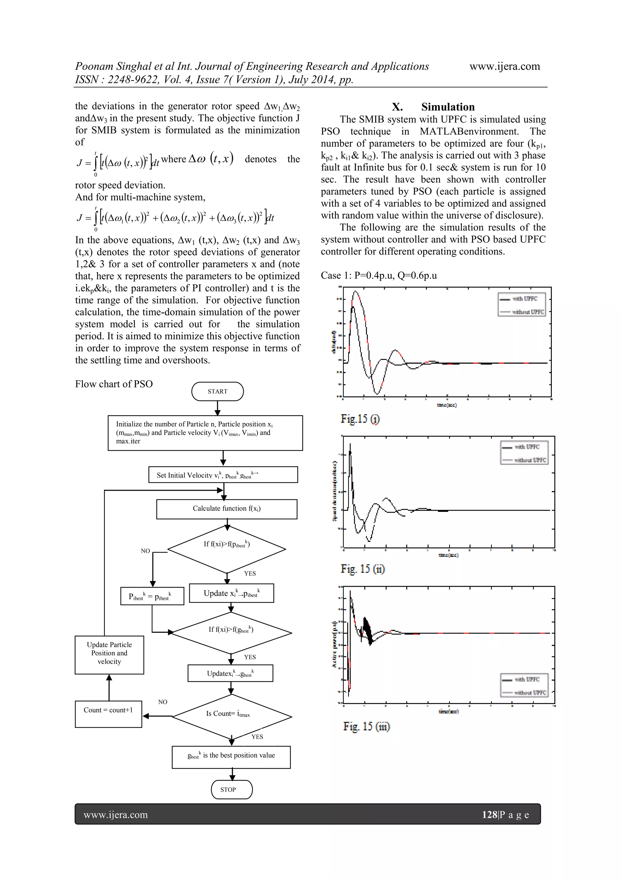
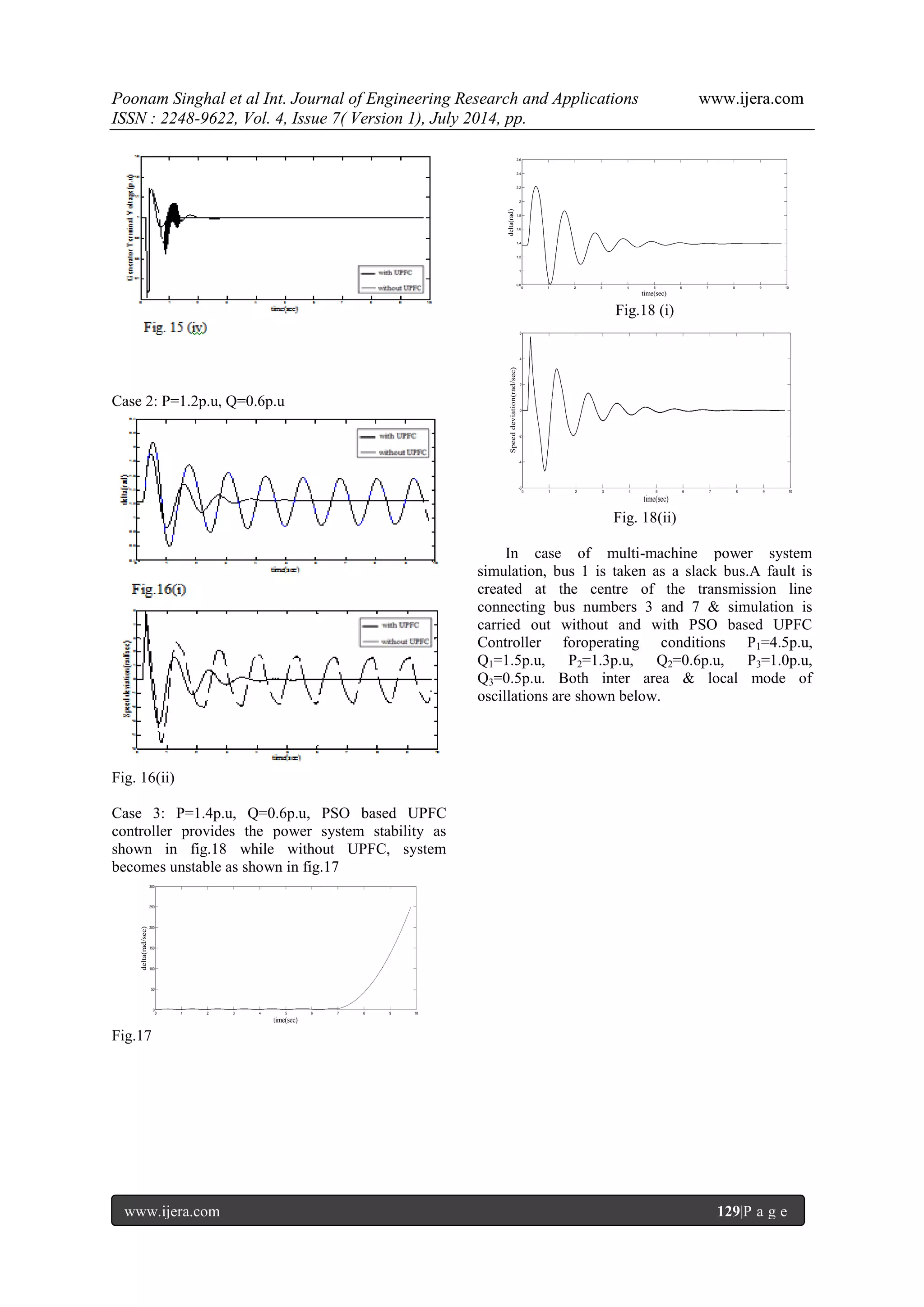
  Poonam Singhal etal Int. Journal of Engineering Research and Applications www.ijera.com ISSN : 2248-9622, Vol. 4, Issue 7( Version 1), July 2014, pp. www.ijera.com 127|P a g e Hence the generator terminal voltage components in the common reference frame and the machine internal voltages are related by   mn m mn m mn m V U T x T Y T E 1 1   Where U is the unity matrix. Both UPFC‟s are represented by an equivalent admittances derived from their power injection models : 2 2 j j j Lj i i j Li V P jQ Y V P jQ Y     Where   i ij i i SH P  B  V sin   V I 2      j ij i j ij P B V V sin  cos  2 i ij i Q  B V       j ij i j ij Q B V V cos When fault is created in any line, the admittance matrix is then modified according to position of fault& taking into account of UPFC admittances. All system equations are converted into common frame of reference which is rotating at synchronous speed. VIII. PARTICLE SWARM OPTIMIZATION BASICS PSO was introduced by Eberhart and kennedy in1995 [22]. It is a heuristic & stochastic based optimization technique. PSO can be used on optimization problem that are partially irregular, noisy, change over time, etc. It is developed from swarm intelligence and is based on the research of bird and fish flock movement behavior .The particle swarm optimization consists of swarm of particles which are initialized with a population of random candidate solution in the multidimensional search space. During their flying movement they follow the trajectory according to their own best flying experience (pbest) & best flying experience of the group (gbest). During this process, each particle modify its position & velocity according to shared information to follow the best trajectory leads to optimum solution & this technique is simple & very few parameters need to be determined. The choice of PSO parameters can have a large impact on optimization performance. Selecting PSO parameters that yield good performance has therefore been the subject of much research. A. Algorithm Step 1: Initialize the number of particles,minimum and maximum limits for the d-dimension search space max m , min m anditmax. Step2: Set initial position of particles k i x Where, x m m m  rand  k i * min max min    Step 3: Set initial velocity vi of particles v v v v  rand  k id * min max min    Where,   max max min v  0.1* m m   min max min v  0.1* m  m Step 4: Select initial pibest k, gbest k Step5: calculate cost function f (xi) taking initial position into consideration. Step 6: If f (xi) > f(pibest k) Then Update the value of xi k by pibest k Else retain the pibest k as pibest k end if; Step 7: If f(pibest k) > f(gbest k) Then Update value of pibest k →gbest k Else go to step 8. step 8: If maximum number of iterations has been done then storegbest k as best position value. Else Increase order of iteration by one. Update particle velocity &position:    k  id k k i k i k i k i v  v  c rand pbest  x  c rand gbest  x  1* 1 2* 2 1 1 1   k i k i k i x x v Where, c1and c2 represents the acceleration factors, rand1 and rand2 represents distributed random numbers between (0,1).First part of equation (1) depicts the previous velocity of the particle, the second part is a positive cognitive component & third part is a positive social component as described in [23]. Repeat Step 4 to step 7 Else if, End. IX. FORMULATION OF AN OBJECTIVE FUNCTION Objective function formulated is based on the optimization parameters. It is worth mentioning that the PIparameters of UPFC are tuned using PSO to minimize the power system oscillations after a disturbance so as to improve the transient stability. These oscillations are reflected in
• 8.
  Poonam Singhal etal Int. Journal of Engineering Research and Applications www.ijera.com ISSN : 2248-9622, Vol. 4, Issue 7( Version 1), July 2014, pp. www.ijera.com 128|P a g e the deviations in the generator rotor speed Δw1,Δw2 andΔw3 in the present study. The objective function J for SMIB system is formulated as the minimization of        t J t t x dt 0 2  , where  t, x denotes the rotor speed deviation. And for multi-machine system,                t J t t x t x t x dt 0 2 3 2 2 2 1  ,  ,  , In the above equations, Δw1 (t,x), Δw2 (t,x) and Δw3 (t,x) denotes the rotor speed deviations of generator 1,2& 3 for a set of controller parameters x and (note that, here x represents the parameters to be optimized i.ekp&ki, the parameters of PI controller) and t is the time range of the simulation. For objective function calculation, the time-domain simulation of the power system model is carried out for the simulation period. It is aimed to minimize this objective function in order to improve the system response in terms of the settling time and overshoots. Flow chart of PSO X. Simulation The SMIB system with UPFC is simulated using PSO technique in MATLABenvironment. The number of parameters to be optimized are four (kp1, kp2 , ki1& ki2). The analysis is carried out with 3 phase fault at Infinite bus for 0.1 sec& system is run for 10 sec. The result have been shown with controller parameters tuned by PSO (each particle is assigned with a set of 4 variables to be optimized and assigned with random value within the universe of disclosure). The following are the simulation results of the system without controller and with PSO based UPFC controller for different operating conditions. Case 1: P=0.4p.u, Q=0.6p.u YES NO NO YES START Initialize the number of Particle n, Particle position xi (mmax,mmin) and Particle velocity Vi (Vimax, Vimin) and max.iter Set Initial Velocity vi k, pbest k ,gbest k→ Calculate function f(xi) If f(xi)>f(pibest k) Update xi k →pibest k If f(xi)>f(gbest k) Updatexi k →gbest k Is Count= itmax gbest k is the best position value STOP Pibest k = pibest k Count = count+1 Update Particle Position and velocity YES
• 9.
  Poonam Singhal etal Int. Journal of Engineering Research and Applications www.ijera.com ISSN : 2248-9622, Vol. 4, Issue 7( Version 1), July 2014, pp. www.ijera.com 129|P a g e Case 2: P=1.2p.u, Q=0.6p.u Fig. 16(ii) Case 3: P=1.4p.u, Q=0.6p.u, PSO based UPFC controller provides the power system stability as shown in fig.18 while without UPFC, system becomes unstable as shown in fig.17 Fig.17 Fig.18 (i) Fig. 18(ii) In case of multi-machine power system simulation, bus 1 is taken as a slack bus.A fault is created at the centre of the transmission line connecting bus numbers 3 and 7 & simulation is carried out without and with PSO based UPFC Controller foroperating conditions P1=4.5p.u, Q1=1.5p.u, P2=1.3p.u, Q2=0.6p.u, P3=1.0p.u, Q3=0.5p.u. Both inter area & local mode of oscillations are shown below. 0 1 2 3 4 5 6 7 8 9 10 0 50 100 150 200 250 300 time(sec) delta(rad/sec) 0 1 2 3 4 5 6 7 8 9 10 0.8 1 1.2 1.4 1.6 1.8 2 2.2 2.4 2.6 time(sec) delta(rad) 0 1 2 3 4 5 6 7 8 9 10 -6 -4 -2 0 2 4 6 time(sec) Speed deviation(rad/sec)
• 10.
  Poonam Singhal etal Int. Journal of Engineering Research and Applications www.ijera.com ISSN : 2248-9622, Vol. 4, Issue 7( Version 1), July 2014, pp. www.ijera.com 130|P a g e z Fig. 19 (iv) Fig. 19 (v) Fig. 19 (vi) 0 5 10 15 20 25 30 35 40 45 50 -0.4 -0.35 -0.3 -0.25 -0.2 -0.15 -0.1 -0.05 0 0.05 time(sec) delta2-delta1(rad) 0 5 10 15 20 25 30 35 40 45 50 -0.45 -0.4 -0.35 -0.3 -0.25 -0.2 -0.15 -0.1 -0.05 0 time(sec) delta3-delta1(rad) 0 5 10 15 20 25 30 35 40 45 50 -0.4 -0.3 -0.2 -0.1 0 0.1 0.2 0.3 time(sec) delta3-delta2(rad)
• 11.
  Poonam Singhal etal Int. Journal of Engineering Research and Applications www.ijera.com ISSN : 2248-9622, Vol. 4, Issue 7( Version 1), July 2014, pp. www.ijera.com 131|P a g e XI. CONCLUSION The UPFC controller parameters (kp1, ki1, kp2, ki2) of UPFC Controller in an SMIB system and (kp1, kp2, kpp1, kpp2 ki1, ki2, kii1, kii2) in multi-machine system are tuned effectively for transient stability enhancement. The response curve shows that the speed deviation, machine angle, generator terminal voltage, active power and reactive power are settled down quickly after the disturbance in an SMIB system and angular speed deviation, rotor angle, & voltage oscillations for inter area (m/c 2 vs. m/c 1 and m/c 3 vs. m/c1) and local area (m/c 3 vs. m/c 2) are damped out effectively during fault in line 3-7 in multi-machine power system. This paper has a vital scope for future studies. Artificial Intelligence Methods like genetic algorithm, Fuzzy Logic technique, ant colony optimization technique and Hybrid BFO-Particle Swarm optimization technique can be used to tune the UPFC controller parameters for better transient stability enhancement. Moreover additional auxiliary signals can be added as a supplementary signals for better transient stability enhancement. APPENDIX Generator Data(All reactance are on 100 MVA base) for SMIB system: Generator Data  ' d x 0.17p.u,  ' q x 0.3p.u,  ' do x 0.15 p.u,  d x 1.9 p.u,  q x 1.6,Tdo‟ = 6.314 p.u, H= 5s Exciter data: KE=50, TE= 0.1s Generator Data (All reactance are on 100 MVA base) for Multi-machine system: Generator 1 xd1 = 0.1468p.u , xd1 ‟ = 0.0608p.u , xq1= 0.0969p.u ,xq ‟=0.0969,Tdo1 ‟ = 8.96, H1=5 Generator 2 xd1 = 0.8958p.u , xd1 ‟ = 0.1198p.u , xq1= 0.8645p.u,xq ‟=0.1969, Tdo1 ‟ = 0.1969, H2=4 Generator 3 xd1 =1.3125p.u, xd1 ‟ = 0.1813p.u, xq1=1.2578 p.u,xq ‟=0.25, Tdo1 ‟ = 0.25, H3=4 Exciter Data: KE1= 25,TE1= 0.05sec,KE2=25, TE2=0.02sec, KE3=25, TE3= 0.06sec Transmission line Data: z24=j0.068, z37=j0.068, z84=jz37, z78=0.1*z37, z45=j0.07, z56=0.1*z45, z61=j0.07 Equivalent Load Reactance: YL5=0, YL6=0, YL7=0, YL8=0, YL1=6.261-j1.044, YL2=0.0877-j0.029, YL3=0.0877-j0.0292, YL4=0.9690-j0.3391 UPFC Data: C = 3500 μF, BSE=142.85siemens, V dc base=31.5 kV PSO based Controller Data for SMIB system: kp1=0.3145, ki1=2.7387, kp2=0.5297, ki2=1.9115 PSO based Controller Data for Multi-machine system: kp1 = 0.045, ki1 =0.3245, kpp1 =0.0511, kii1 =0.2211 kp2=0.015,ki2=0.1021, kpp2=0.0115, kii2=0.3101 PSO Parameters: 0 1 2 3 4 5 6 7 8 9 10 -0.01 0 0.01 0.02 0.03 0.04 0.05 time(sec) VSEP1(p.u0 M/c1 0 1 2 3 4 5 6 7 8 9 10 -0.06 -0.05 -0.04 -0.03 -0.02 -0.01 0 time(sec) VSEP2(p.u) M/c1
• 12.
  Poonam Singhal etal Int. Journal of Engineering Research and Applications www.ijera.com ISSN : 2248-9622, Vol. 4, Issue 7( Version 1), July 2014, pp. www.ijera.com 132|P a g e c1=0.2,c2=0.4, Number of Particles=30,wmax=0.5, wmin=-0.5 References [1] N. G. Hingorani, L. Gyugyi, “Understanding FACTS”, IEEE Press, 2001. [2] P. Kundur, “Power System Stability and Control”, Tata McGraw-Hill, 2006. [3] Y. H. Song, A. T. Johns, “Flexible AC Transmission Systems (FACTS)”, IET, 2009. [4] Power System control & Stability by P.M Anderson & A.A. Foaud. [5] Ali Ajami, S H Hosseini, G B Gharehpetian, “Modelling and Controlling of UPFC for power system transient studies”, ECTI Transations on Electrical Eng., Electronics, And Communications Vol.5, No.2, August 2007. [6] L.Gyugi, C.D. Schauder, “Unified Power Flow Controller: A New Approach To Power Transmission Control:, IEEE Transactions on Power Delivery, Vol.10, No.2, pp 1085-1093, April 1995. [7] H.Fujita, Y.Watanabe, H.Akagi,”Control and Analysis of Unified Power Flow Controller”, IEEE Transaction on Power Electronics, Vol.14, No.6, pp. 1021-1027, November 1999. [8] Pranesh Rao. M. L. Crow, Zhiping Yang, “STATCOM Control for Power System Voltage Control Applications”, IEEE Transaction on Power Delivery, Vol 15, No.4, pp 1311-1317, October 2000 [9] S.H. Hosseini, A. Ajami, “Transient StabilityEnhancement of AC Trasmission System UsingSTATCOM," TENCON'02, October 2002BeijingChina [10] L. Gyugyi, C.D. Schauder, K.K. Sen, “Static Synchronous Series Compensator: A Solid- State Approach to the Series Compensation of Trasmission Line”, IEEE Transactions on on Power Delivery, Vol. 12, No. 1, pp. 406- 413,1997 [11] S.H. Hosseini, A. Ajami, “Dynamic Compensation of Power System Using a Mulilevel Sataic Synchronous Series Compensator”, 8th International Iranian Conference on Electrical Engineering May 2000 [12] A. Nabavi-Niaki, M. R. Iravani, “Steady State and Dynamic Models of Unified Power Flow Controller for Power System Studies,” IEEE Transactions on Power System, Vol. 11, No. 4, November 1996, pp. 1937-1943 [13] C.Shauder and H.Mehta, “Vector analysis and control of advanced static VAR compensators”, IEE Proc, 140, No. 4, July 1993 [14] R. Mihalic et. al., “Improvement of Transient Stability Using Unified power Flow Controller,” IEEE Transactions on Power Delivery, Vol. 11, No. 1, January 1996, pp. 485-492 [15] S. Limyingcharoen, U.D. Annakkage and N.C.Pahalawaththa, “Effects of Unified Power FlowController on Transient Stability,” IEE Proc.Gener. Transm. Distrib., Vol. 145, No. 2, March 1998, pp. 182-188 [16] Poonam Singhal, S. K. Agarwaland Narender Kumar,”Optimization of UPFCController ParametersUsing BacterialForaging Technique forEnhancing Power System Stability”,Vol.5.No.2 (March2014),IJOAT. [17] Mahmoud H. M, M. A. Mehanna and S. K. Elsayed, “Optimal Location of Facts Devices to Enhance the Voltage Stability and Power Transfer Capability”, Journal of American Science, 2012. [18] Theja,B.S. ; Rajasekhar, A. ; Kothari, D.P., “An intelligent coordinated design of UPFC based power system stabilizer for dynamic stabilityenhancement of SMIB power system” IEEE International Conference on Power Electronics, Drives and Energy Systems (PEDES), 2012 [19] Flexible AC Transmission Systems(FACTS), by Yong Hua Song & Allan T.Johns. [20] Poonam Singhal,S.K.Agarwal & Narender Kumar,”Transient Analysis Enhancement of a Power System using Unified Power flow controller,IREMOS, Volume 6,no5,Dec2013. [21] Poonam Singhal,S.K.Agarwal & NarenderKumar,”StabilityEnhancement of a Multi-Machine Power System using Static VAR Compensator.IJAIR, Vol2,Issue2,2013. [22] J. Kennedy and R. Eberhart, “Particle swarm optimization,” in Proc.IEEE Int. Conf. Neural Networks, 1995, pp. 1942– 1948., [23] Asanga Ratanweera, Saman k. Halgamuge, Harry C. Watson,”Self Organising Hierarchical Particle Swarm Optimizater with time-varying Acceleration Coefficient [24] Sedraoui, K.; Fnaiech, F.; Al-Haddad, K., “Solutions for Power Quality Using the Advanced UPFC - Control Strategy and Case Study”IREE Volume: 3 , Issue: 5, pp. 811-819, Sept-Oct, 2008 [25] Iraj Rahimi Pordanjani, Hooman Efranian Mazin, Gevorg B. Gharehpetian, “Effects of STATCOM, TCSC, SSSC and UPFC on Static Voltage Stability”IREE Volume: 4 , Issue: 4, part B, pp. 1376-1384, Nov-Dec, 200f9
• 13.
  Poonam Singhal etal Int. Journal of Engineering Research and Applications www.ijera.com ISSN : 2248-9622, Vol. 4, Issue 7( Version 1), July 2014, pp. www.ijera.com 133|P a g e [26] A.nabavi Niaki and M.R.Iravani “Steady- State and Dynamic Models of UPFC for Power System Studies”IEEE Transactions on power systems,vol 11,.no.4,Nov1996 [27] N.Dizdarevic and G.Andersson“Power Flow regulation by use of UPFC’s Injection model” Authors’ information 1Associate Professor, Deptt. of Electrical Engineering, YMCAUST, Faridabad, India. 2Professor and Head, Deptt.of Electronics Engineering, YMCAUST, Faridabad, India. 3Professor, Deptt. of Electrical Engineering, DTU, Delhi, India. 4Assistant Professor, Deptt. of EEE, MAIT, Delhi, India. Poonam Singhalwas born in 1964.She is currently Associate Professor in YMCA UniversityofScience& Technology, Faridabad, Haryana (India).She did her B.ScEngg from REC Rourkela,Odisha (India)&M.Tech (Power System & Drives) from YMCA University of Science &Technology, Faridabad, Haryana (India). Her main area of interest are FACTS, Power System Operation control & Simulation. S. K Agarwalwas born in 1961. He is currently Professor in Department of Electronics Engineering, YMCA University of Science &Technology, Faridabad and Haryana (India) .He did his B.Tech from REC Calicut,Kerala(India) & M.E. (Controls & Instrumentation) from Delhi Technological University Delhi(India) &Ph.D from JamiaMiliaIslamia University Delhi(India). Prof. S. K. Agarwal has many publications in National/International Journals & presented papers in International conferences. Prof.Agarwal‟s main area of interest are Power System & Controls. Narender Kumarwas born in Aligarh(India). He received his B.Sc.Engg.& M.Sc. Engg in Electrical Engineering from A.M.U. Aligarh in 1984 & 1986 respectively. Presently, he is Professor of Electrical Engg. in Delhi Technological University, Delhi. Prof.Narender Kumar has published various papers in national and international conferences and journals. Prof.NarenderKumar‟s main area of interest are Power System Operation Control &Simulation,SSR,and AGC etc.