Download to read offline


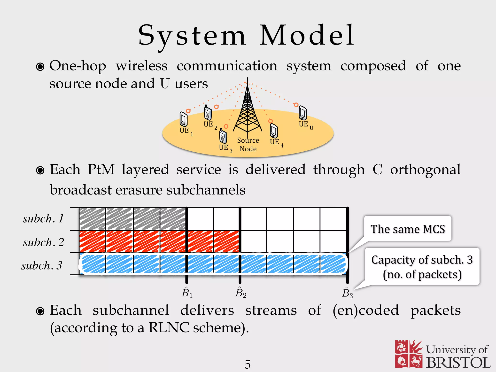
![6 ๏ Encoding performed over each service layer independently from the others. ๏ The source node will linearly combine the data packets composing the l-th layer and will generate a stream of coded packets, where ๏ is a layered source message of K source packets, classified into L service layers x = {x1, . . . , xK} RNC in a Nutshell kl Coef:icients of the linear combination are selected over a :inite :ield of size q {xi}K` i=K` 1+1 yj = K`X i=K` 1+1 cj,i · xi k1 k2 k3 K3 = K K2 K1 x1 x2 . . .. . . xK Fig. 1. Layered source message, in the case of L = 3. the scope of the paper to provide analytical and optimization frameworks dealing with the compression strategy used to generate a scalable service. For these reasons, the proposed analysis has been made independent of the way service layers are generated and the nature of the adopted service scalability. As suggested in [12], [18], we model the transmitted service use rec tha SR an ide pa of sys is to sys](https://image.slidesharecdn.com/uobsparse-151012141945-lva1-app6892/75/Sparse-Random-Network-Coding-for-Reliable-Multicast-Services-6-2048.jpg)
![RNC in a Nutshell ๏ When has rank equal to , the user can keep only the linearly independent rows and invert the matrix. 8 Cu n` k` Encoding Decoding Cu · xT ` = yT () C 1 u · yT ` = xT ` ๏ Given [1, 0] and [0, 1], is [2, 2] linearly independent? ✴ No, because 2[1, 0] + 2[0, 1] - [2, 2] = [0, 0] ๏ Given two lin. indep. vectors (a and b) in GF(q), how many vectors form span({a,b})? ✴ q2. For a = [1, 0], b = [0, 1] and q = 2, span({a,b}) = {[0, 0],
[0, 1], [1, 0], [1, 1]]} ๏ Let us encode over a set of 5 inf. elements, if I collected 3 lin. indep. coding vectors, what is the prob. of collecting a new lin. dep. coding vec.? ✴ q3 / q5](https://image.slidesharecdn.com/uobsparse-151012141945-lva1-app6892/75/Sparse-Random-Network-Coding-for-Reliable-Multicast-Services-8-2048.jpg)

![The Coding Matrix ๏ Matrix is a random matrix over GF(q), where elements are independently and uniformly selected by the following prob. law 10 Cu ๏ If , all the GF(q) elements are equiprobable and things are nice and easy… otherwise, things get tricky! ๏ Since 1997, only 2 conference papers and 2 (+1 on Arxiv) journal papers deal with sparse random matrices. cupied vide an mission ice. of K essage. ber kℓ e MCS service e block (mℓ)⌉. source nd are cement ize the ill also parsity mized. the transmission of each layer shall meet a temporal constraint. The sparse versions of both the classic (S-RLNC) and systematic implementation of RLNC (S-SRLNC) are obtained as follows. Each component cj,i of a non-degenerate coding vector associated with source message layer ℓ is independently and identically distributed as follows [25]: Pr (cj,i = v) = ⎧ ⎨ ⎩ pℓ if v = 0 1 − pℓ q − 1 if v ∈ GF(q) {0} (1) where pℓ, for 0 < pℓ < 1, is the probability of having cj,i = 0. The event cj,i ̸= 0 occurs with probability 1 − pℓ. We remark that the average number of source packets involved in the generation of a non-degenerate coded packet, i.e., the sparsity of the code, can be controlled by tuning the value of pℓ, for any ℓ = 1, . . . , L. Since coding vectors are generated at random, there is the possibility of generating coding vectors where each coding coefficient is equal to 0. From a system implementation p` = 1/q](https://image.slidesharecdn.com/uobsparse-151012141945-lva1-app6892/75/Sparse-Random-Network-Coding-for-Reliable-Multicast-Services-10-2048.jpg)

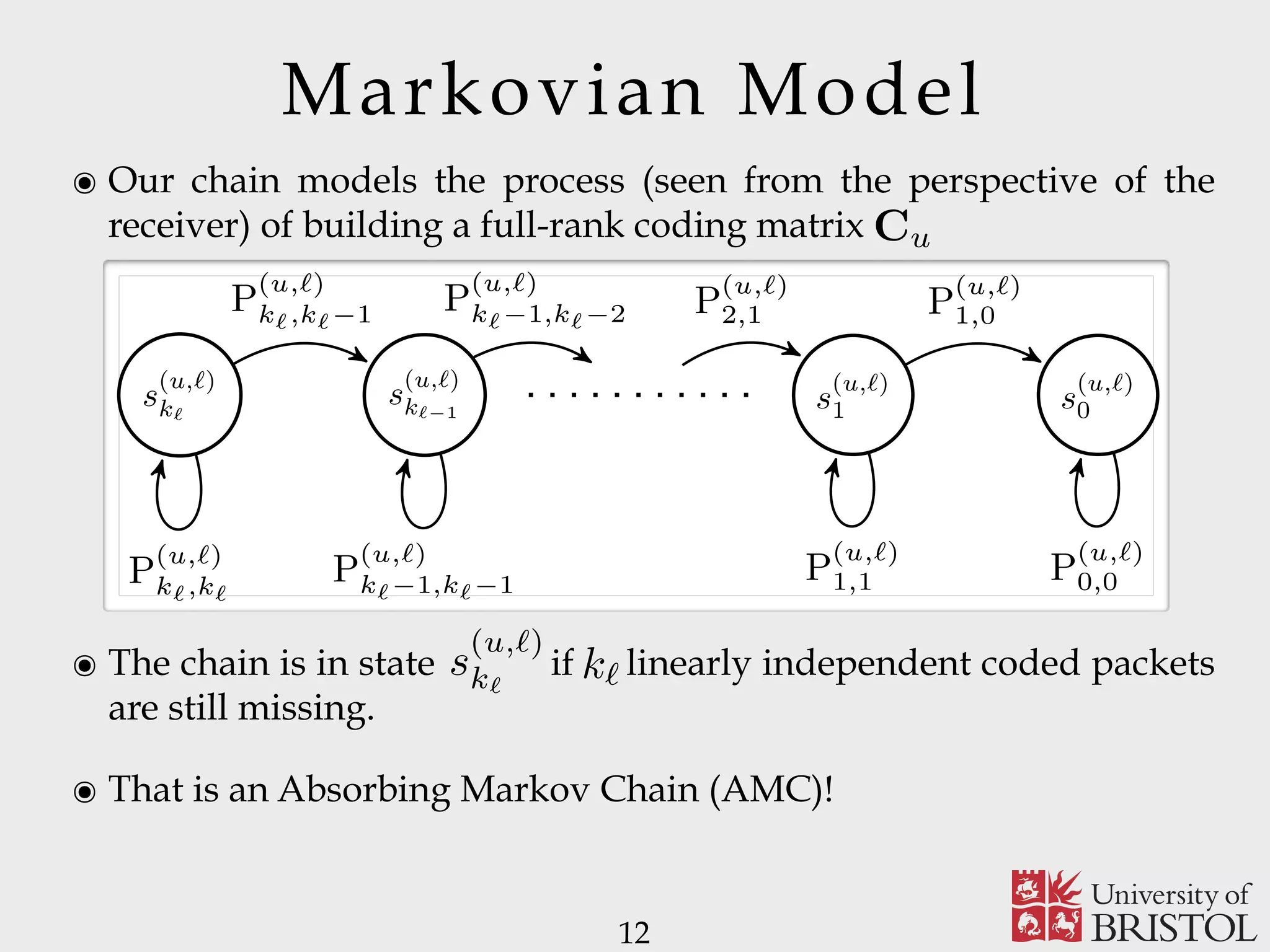
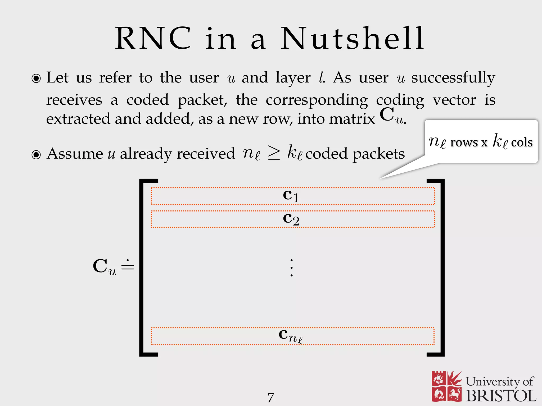
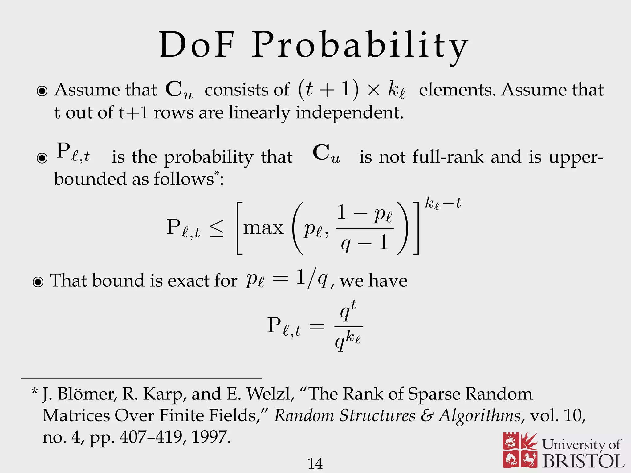
![Markovian Model 13 5 rch of ich on, del In MC. ing u ℓ, s a s (u,ℓ) kℓ s (u,ℓ) kℓ−1 s (u,ℓ) 1 s (u,ℓ) 0 P (u,ℓ) kℓ,kℓ P (u,ℓ) kℓ,kℓ−1 P (u,ℓ) kℓ−1,kℓ−1 P (u,ℓ) kℓ−1,kℓ−2 P (u,ℓ) 2,1 P (u,ℓ) 1,1 P (u,ℓ) 1,0 P (u,ℓ) 0,0 Fig. 2. State transition diagram for the AMC associated with user u and message layer ℓ. paper, owing to the lack of the exact expression of Pℓ,t, we use (2) to approximate Pℓ,t, that is Pℓ,t ∼= max pℓ, 1 − pℓ q − 1 kℓ−t . (3) mes- , kℓ. t or fect The MC are ave rder we nted Cu 1), ent. the clearly not applicable to the sparse case, in contrast to (3). It is worth mentioning that the considered approximation (3) collapses to the exact expression of Pℓ,t and, hence, the relation Pℓ,t = [max (pℓ, (1 − pℓ)/(q − 1))]kℓ−t = qt /qk ℓ holds, for pℓ = q−1 . From (3), the transition probability matrix describing the AMC associated with user u and message layer ℓ can be derived by the following lemma. Lemma 2.2: Assume layer ℓ is transmitted over a subchannel which adopts the MCS with index m. The probability P (u,ℓ) i,j of moving from state s (u,ℓ) i to state s (u,ℓ) j is P (u,ℓ) i,j = ⎧ ⎨ ⎩ (1 − Pℓ,kℓ−i)[1 − pu(m)] if i − j = 1 Pℓ,kℓ−i[1 − pu(m)] + pu(m) if i = j 0 otherwise. (4) Proof: Since the user AMC is in state s (u,ℓ) i , user u has collected kℓ − i linearly independent coded packets, i.e., User PER for a given MCS m Unknown! We used an upper-bound!](https://image.slidesharecdn.com/uobsparse-151012141945-lva1-app6892/75/Sparse-Random-Network-Coding-for-Reliable-Multicast-Services-13-2048.jpg)
![Markovian Model 15 5 rch of ich on, del In MC. ing u ℓ, s a s (u,ℓ) kℓ s (u,ℓ) kℓ−1 s (u,ℓ) 1 s (u,ℓ) 0 P (u,ℓ) kℓ,kℓ P (u,ℓ) kℓ,kℓ−1 P (u,ℓ) kℓ−1,kℓ−1 P (u,ℓ) kℓ−1,kℓ−2 P (u,ℓ) 2,1 P (u,ℓ) 1,1 P (u,ℓ) 1,0 P (u,ℓ) 0,0 Fig. 2. State transition diagram for the AMC associated with user u and message layer ℓ. paper, owing to the lack of the exact expression of Pℓ,t, we use (2) to approximate Pℓ,t, that is Pℓ,t ∼= max pℓ, 1 − pℓ q − 1 kℓ−t . (3) as transient states [35]. The state transition diagram of th resulting AMC can be represented as reported in Fig. 2. From Lemma 2.2, it directly follows that th (kℓ + 1) × (kℓ + 1) transition matrix T(u,ℓ) describing the AMC of user u and associated with layer ℓ has th following structure in its canonical form [35]: T(u,ℓ) . = 1 0 R(u,ℓ) Q(u,ℓ) , (5 where Q(u,ℓ) is the kℓ × kℓ transition matrix modeling th AMC process as long as it involves only transient states. Th term R(u,ℓ) is a column vector of kℓ elements which lists al the probabilities of moving from a transient to the absorbing (u,ℓ) AMC transition matrix resulting AMC can be represented as reported in Fig. 2. From Lemma 2.2, it directly follows that the (kℓ + 1) × (kℓ + 1) transition matrix T(u,ℓ) describing the AMC of user u and associated with layer ℓ has the following structure in its canonical form [35]: T(u,ℓ) . = 1 0 R(u,ℓ) Q(u,ℓ) , (5) where Q(u,ℓ) is the kℓ × kℓ transition matrix modeling the AMC process as long as it involves only transient states. The term R(u,ℓ) is a column vector of kℓ elements which lists all the probabilities of moving from a transient to the absorbing state. From [35, Theorem 3.2.4], let define matrix N(u,ℓ) as N(u,ℓ) = ∞ t=0 Q(u,ℓ) t = I − Q(u,ℓ) −1 . (6) Element N (u,ℓ) i,j at the location (i, j) of matrix N(u,ℓ) defines Fundamental matrix](https://image.slidesharecdn.com/uobsparse-151012141945-lva1-app6892/75/Sparse-Random-Network-Coding-for-Reliable-Multicast-Services-15-2048.jpg)
![Markovian Model ๏ Why is the fundamental matrix so important? Its (i,j) element is the avg. number of coded packet transmissions needed (to a system started at the i-th state) to get to the j-th state. ๏ Hence, the avg number of transmissions needed to get to the absorbing state (for a system started in the i-th state) is 16 i,j the average number of coded packet transmissions required for the process transition from state s (u,ℓ) i to state s (u,ℓ) j , where both s (u,ℓ) i and s (u,ℓ) j are transient states. In particular, from Lemma 2.2, the following theorem holds Theorem 2.1 ([35, Theorem 3.3.5]): If the AMC is in the transient state s (u,ℓ) i , the average number of coded packet transmissions needed to get to state s (u,ℓ) 0 is τ (u,ℓ) i = ⎧ ⎪⎨ ⎪⎩ 0 if i = 0 i j=1 N (u,ℓ) i,j if i = 1, . . . , kℓ. (7) From (7) and Theorem 2.1, we prove the following corollaries. Corollary 2.1: In the case of S-RLNC, the average number τ (u,ℓ) S-RLNC of coded packets transmissions needed by user u to recover the source message layer ℓ is τ (u,ℓ) = τ (u,ℓ) . ๏ In the non-systematic RNC we have 5, Theorem 3.3.5]): If the AMC is in the ) , the average number of coded packet d to get to state s (u,ℓ) 0 is 0 if i = 0 i j=1 N (u,ℓ) i,j if i = 1, . . . , kℓ. (7) em 2.1, we prove the following corollaries. the case of S-RLNC, the average number ackets transmissions needed by user u to message layer ℓ is τ (u,ℓ) S-RLNC = τ (u,ℓ) kℓ . the source node transmits the very first (u,ℓ) simply a value of III. S Amon putation consider increase per sou remark increase resource](https://image.slidesharecdn.com/uobsparse-151012141945-lva1-app6892/75/Sparse-Random-Network-Coding-for-Reliable-Multicast-Services-16-2048.jpg)

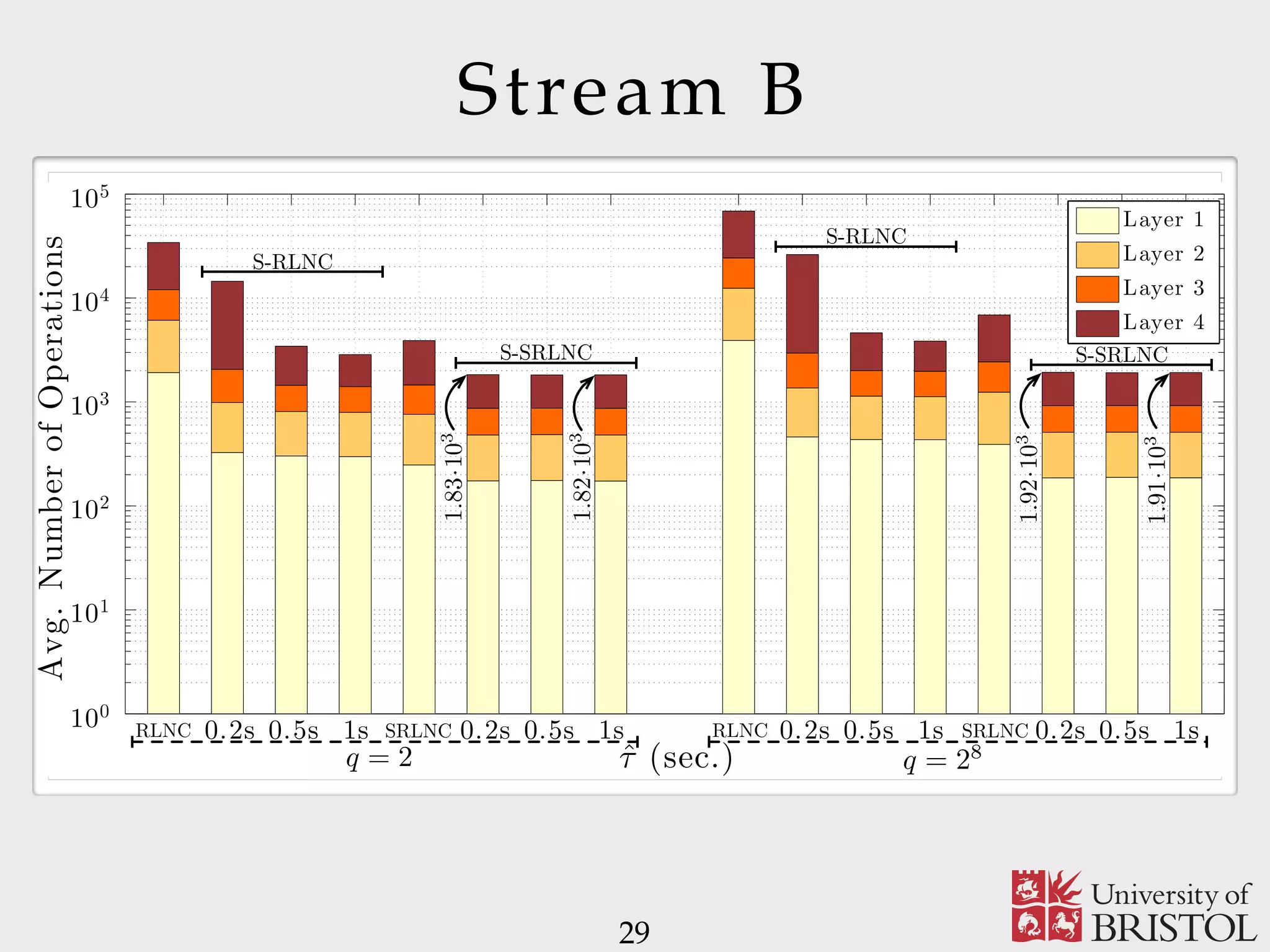


The document discusses Sparse Random Network Coding (RNCC) for reliable multicast services in communication systems, emphasizing the computational complexity of RNCC decoders and proposing methods to optimize transmission parameters and sparsity. It presents a Markov chain performance analysis to model the process of coding matrix formation and provides numerical results for various implementations. The findings suggest that controlling sparsity improves decoding efficiency while maintaining battery life in mobile devices.