Introduction Reliability ofa software product: a concern for most users especially industry users. An important attribute determining the quality of the product. Users not only want highly reliable products: want quantitative estimation of reliability before making buying decision.
4.
Introduction Accurate measurementof software reliability: a very difficult problem Several factors contribute to making measurement of software reliability difficult.
5.
Major Problems inReliability Measurements Errors do not cause failures at the same frequency and severity. measuring latent errors alone not enough The failure rate is observer- dependent
6.
Software Reliability: 2 AlternateDefinitions Informally denotes a product’s trustworthiness or dependability. Probability of the product working “correctly” over a given period of time.
7.
Software Reliability Intuitively: asoftware product having a large number of defects is unreliable. It is also clear: reliability of a system improves if the number of defects is reduced.
8.
Difficulties in Software ReliabilityMeasurement (1) No simple relationship between: observed system reliability and the number of latent software defects. Removing errors from parts of software which are rarely used: makes little difference to the perceived reliability.
9.
The 90-10 Rule Experiments from analysis of behavior of a large number of programs: 90% of the total execution time is spent in executing only 10% of the instructions in the program. The most used 10% instructions: called the core of the program.
10.
Effect of 90-10Rule on Software Reliability Least used 90% statements: called non-core are executed only during 10% of the total execution time. It may not be very surprising then: removing 60% defects from least used parts would lead to only about 3% improvement to product reliability.
11.
Difficulty in Software ReliabilityMeasurement Reliability improvements from correction of a single error: depends on whether the error belongs to the core or the non- core part of the program.
12.
Difficulty in Software ReliabilityMeasurement (2) The perceived reliability depends to a large extent upon: how the product is used, In technical terms on its operation profile.
13.
Effect of OperationalProfile on Software Reliability Measurement If we select input data: only “correctly” implemented functions are executed, none of the errors will be exposed perceived reliability of the product will be high.
14.
Effect of OperationalProfile on Software Reliability Measurement On the other hand, if we select the input data: such that only functions containing errors are invoked, perceived reliability of the system will be low.
15.
Software Reliability Differentusers use a software product in different ways. defects which show up for one user, may not show up for another. Reliability of a software product: clearly observer-dependent cannot be determined absolutely.
16.
Difficulty in Software ReliabilityMeasurement (3) Software reliability keeps changing through out the life of the product Each time an error is detected and corrected
17.
Hardware vs. Software Reliability Hardware failures: inherently different from software failures. Most hardware failures are due to component wear and tear: some component no longer functions as specified.
18.
Hardware vs. Software Reliability A logic gate can be stuck at 1 or 0, or a resistor might short circuit. To fix hardware faults: replace or repair the failed part.
19.
Hardware vs. Software Reliability Software faults are latent: system will continue to fail: unless changes are made to the software design and code.
20.
Hardware vs. Software Reliability Because of the difference in effect of faults: Though many metrics are appropriate for hardware reliability measurements Are not good software reliability metrics
21.
Hardware vs. Software Reliability When a hardware is repaired: its reliability is maintained When software is repaired: its reliability may increase or decrease.
22.
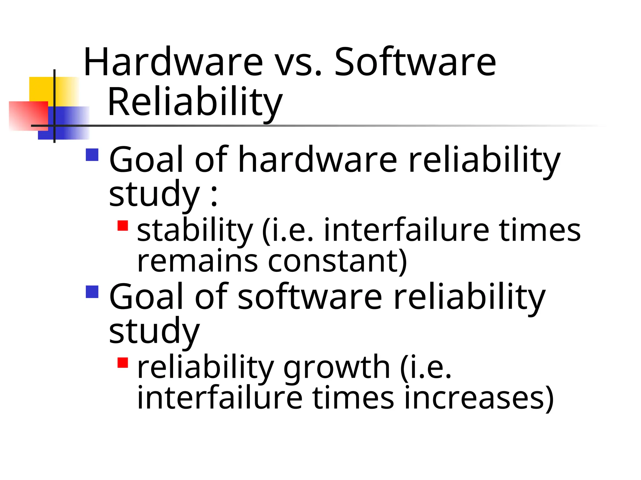
Hardware vs. Software Reliability Goal of hardware reliability study : stability (i.e. interfailure times remains constant) Goal of software reliability study reliability growth (i.e. interfailure times increases)
Reliability Metrics Differentcategories of software products have different reliability requirements: level of reliability required for a software product should be specified in the SRS document.
25.
Reliability Metrics Agood reliability measure should be observer- independent, so that different people can agree on the reliability.
26.
Rate of occurrenceof failure (ROCOF): ROCOF measures: frequency of occurrence failures. observe the behavior of a software product in operation: over a specified time interval calculate the total number of failures during the interval.
27.
Mean Time ToFailure (MTTF) Average time between two successive failures: observed over a large number of failures.
28.
Mean Time ToFailure (MTTF) MTTF is not as appropriate for software as for hardware: Hardware fails due to a component’s wear and tear thus indicates how frequently the component fails When a software error is detected and repaired: the same error never appears.
29.
Mean Time ToFailure (MTTF) We can record failure data for n failures: let these be t1, t2, …, tn calculate (ti+1-ti) the average value is MTTF (ti+1-ti)/(n-1)
30.
Mean Time toRepair (MTTR) Once failure occurs: additional time is lost to fix faults MTTR: measures average time it takes to fix faults.
31.
Mean Time BetweenFailures (MTBF) We can combine MTTF and MTTR: to get an availability metric: MTBF=MTTF+MTTR MTBF of 100 hours would indicae Once a failure occurs, the next failure is expected after 100 hours of clock time (not running time).
32.
Probability of Failureon Demand (POFOD) Unlike other metrics This metric does not explicitly involve time. Measures the likelihood of the system failing: when a service request is made. POFOD of 0.001 means: 1 out of 1000 service requests may result in a failure.
33.
Availability Measures howlikely the system shall be available for use over a period of time: considers the number of failures occurring during a time interval, also takes into account the repair time (down time) of a system.
34.
Availability This metricis important for systems like: telecommunication systems, operating systems, etc. which are supposed to be never down where repair and restart time are significant and loss of service during that time is important.
35.
Reliability metrics Allreliability metrics we discussed: centered around the probability of system failures: take no account of the consequences of failures. severity of failures may be very different.
36.
Reliability metrics Failureswhich are transient and whose consequences are not serious: of little practical importance in the use of a software product. such failures can at best be minor irritants.
37.
Failure Classes Moresevere types of failures: may render the system totally unusable. To accurately estimate reliability of a software product: it is necessary to classify different types of failures.
38.
Failure Classes Transient: Transientfailures occur only for certain inputs. Permanent: Permanent failures occur for all input values. Recoverable: When recoverable failures occur: the system recovers with or without operator intervention.
39.
Failure Classes Unrecoverable: the system may have to be restarted. Cosmetic: These failures just cause minor irritations, do not lead to incorrect results. An example of a cosmetic failure: mouse button has to be clicked twice instead of once to invoke a GUI function.
40.
Reliability Growth Modelling A reliability growth model: a model of how software reliability grows as errors are detected and repaired. A reliability growth model can be used to predict: when (or if at all) a particular level of reliability is likely to be attained. i.e. how long to test the system?
41.
Reliability Growth Modelling There are two main types of uncertainty: in modelling reliability growth which render any reliability measurement inaccurate: Type 1 uncertainty: our lack of knowledge about how the system will be used, i.e. its operational profile
42.
Reliability Growth Modelling Type 2 uncertainty: reflects our lack of knowledge about the effect of fault removal. When we fix a fault we are not sure if the corrections are complete and successful and no other faults are introduced Even if the faults are fixed properly we do not know how much will be the improvement to interfailure time.
43.
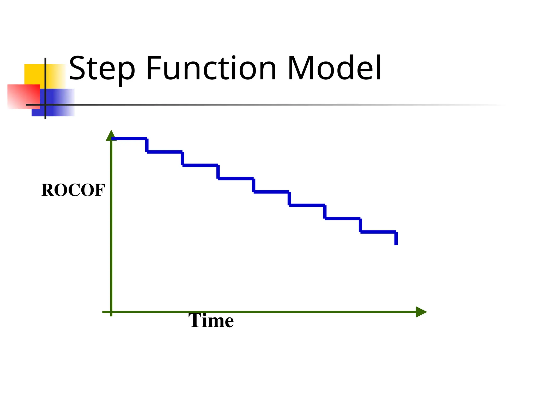
Step Function Model The simplest reliability growth model: a step function model The basic assumption: reliability increases by a constant amount each time an error is detected and repaired.
Step Function Model Assumes: all errors contribute equally to reliability growth highly unrealistic: we already know that different errors contribute differently to reliability growth.
46.
Jelinski and MorandaModel Realizes each time an error is repaired: reliability does not increase by a constant amount. Reliability improvement due to fixing of an error: assumed to be proportional to the number of errors present in the system at that time.
47.
Jelinski and MorandaModel Realistic for many applications, still suffers from several shortcomings. Most probable failures (failure types which occur frequently): discovered early during the testing process.
48.
Jelinski and MorandaModel Repairing faults discovered early: contribute maximum to the reliability growth. Rate of reliability growth should be large initially: slow down later on, contrary to assumption of the model
49.
Littlewood and Verall’sModel Allows for negative reliability growth: when software repair introduces further errors. Models the fact that as errors are repaired: average improvement in reliability per repair decreases.
50.
Littlewood and Verall’sModel Treats a corrected bug’s contribution to reliability improvement: an independent random variable having Gamma distribution. Removes bugs with large contributions to reliability: earlier than bugs with smaller contribution represents diminishing return as test continues.
51.
Reliability growth models There are more complex reliability growth models, more accurate approximations to the reliability growth. these models are out of scope of our discussion.
52.
Applicability of ReliabilityGrowth Models There is no universally applicable reliability growth model. Reliability growth is not independent of application.
53.
Applicability of ReliabilityGrowth Models Fit observed data to several growth models. Take the one that best fits the data.
54.
Statistical Testing Atesting process: the objective is to determine reliability rather than discover errors. uses data different from defect testing.
55.
Statistical Testing Differentusers have different operational profile: i.e. they use the system in different ways formally, operational profile: probability distribution of input
56.
Operational profile: Example An expert user might give advanced commands: use command language interface, compose commands A novice user might issue simple commands: using iconic or menu-based interface.
57.
How to defineoperational profile? Divide the input data into a number of input classes: e.g. create, edit, print, file operations, etc. Assign a probability value to each input class: a probability for an input value from that class to be selected.
58.
Steps involved inStatistical testing (Step-I) Determine the operational profile of the software: This can be determined by analyzing the usage pattern.
59.
Step 2 inStatistical testing Manually select or automatically generate a set of test data: corresponding to the operational profile.
60.
Step 3 inStatistical testing Apply test cases to the program: record execution time between each failure it may not be appropriate to use raw execution time
61.
Step 4 inStatistical testing After a statistically significant number of failures have been observed: reliability can be computed.
62.
Statistical Testing Relieson using large test data set. Assumes that only a small percentage of test inputs: likely to cause system failure.
63.
Statistical Testing Itis straight forward to generate tests corresponding to the most common inputs: but a statistically significant percentage of unlikely inputs should also be included. Creating these may be difficult: especially if test generators are used.
64.
Advantages of Statistical Testing Concentrate on testing parts of the system most likely to be used: results in a system that the users find more reliable (than actually it is!).
65.
Advantages of Statistical Testing Reliability predictions based on test results: gives an accurate estimation of reliability (as perceived by the average user) compared to other types of measurements.
66.
Disadvantages of Statistical Testing It is not easy to do statistical testing properly: there is no simple or repeatable way to accurately define operational profiles. Statistical uncertainty.