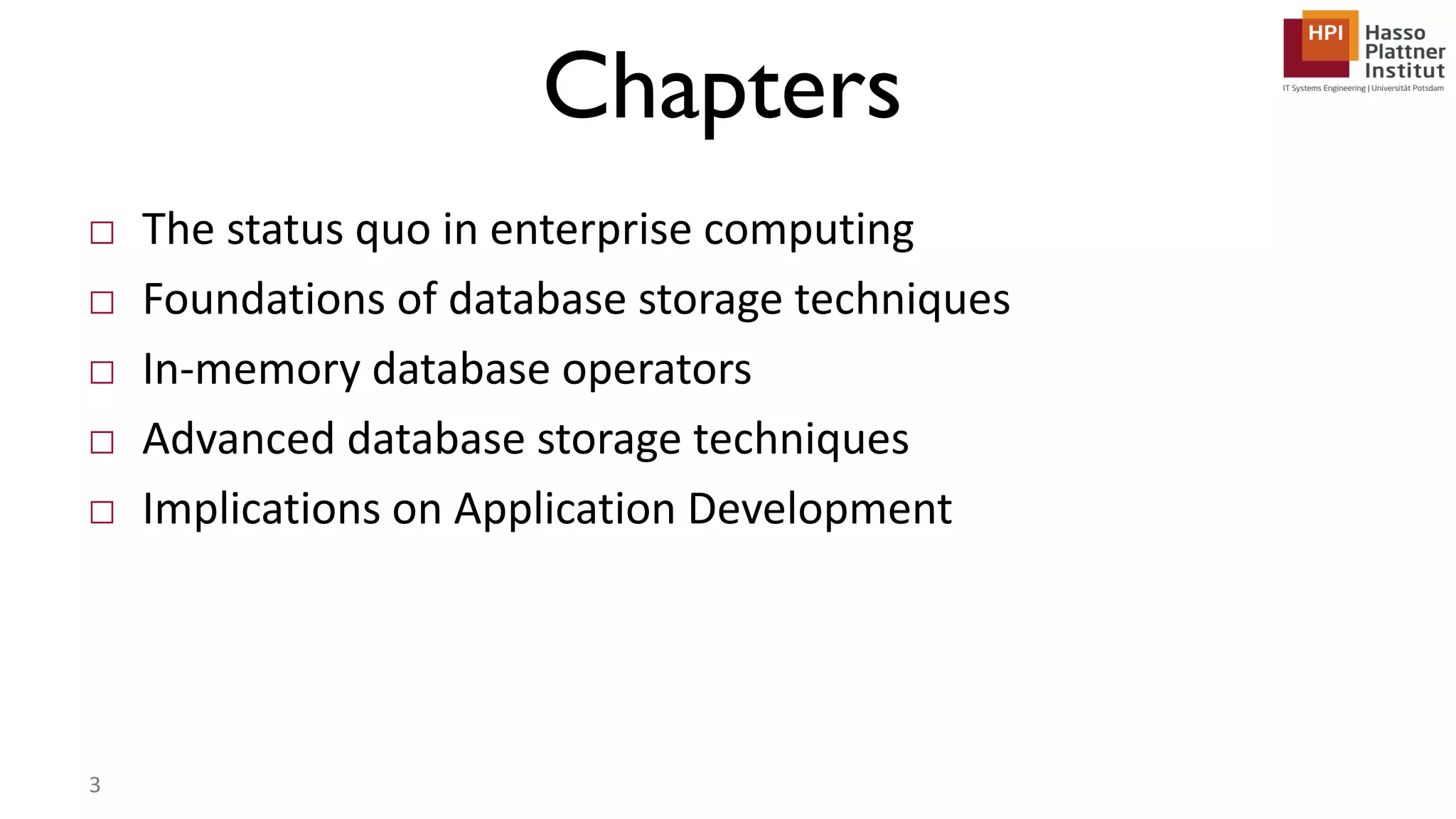
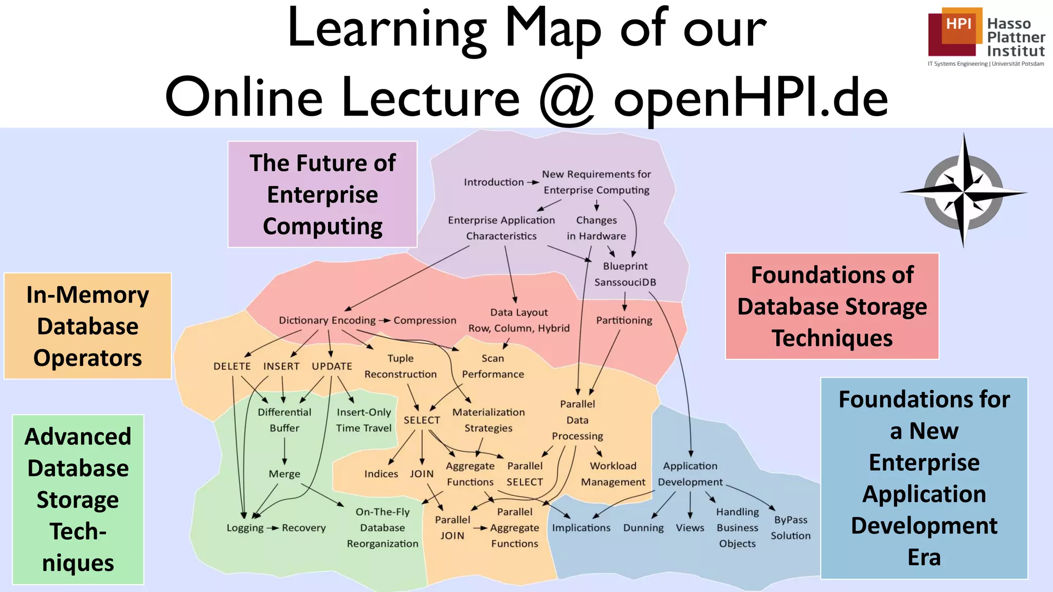
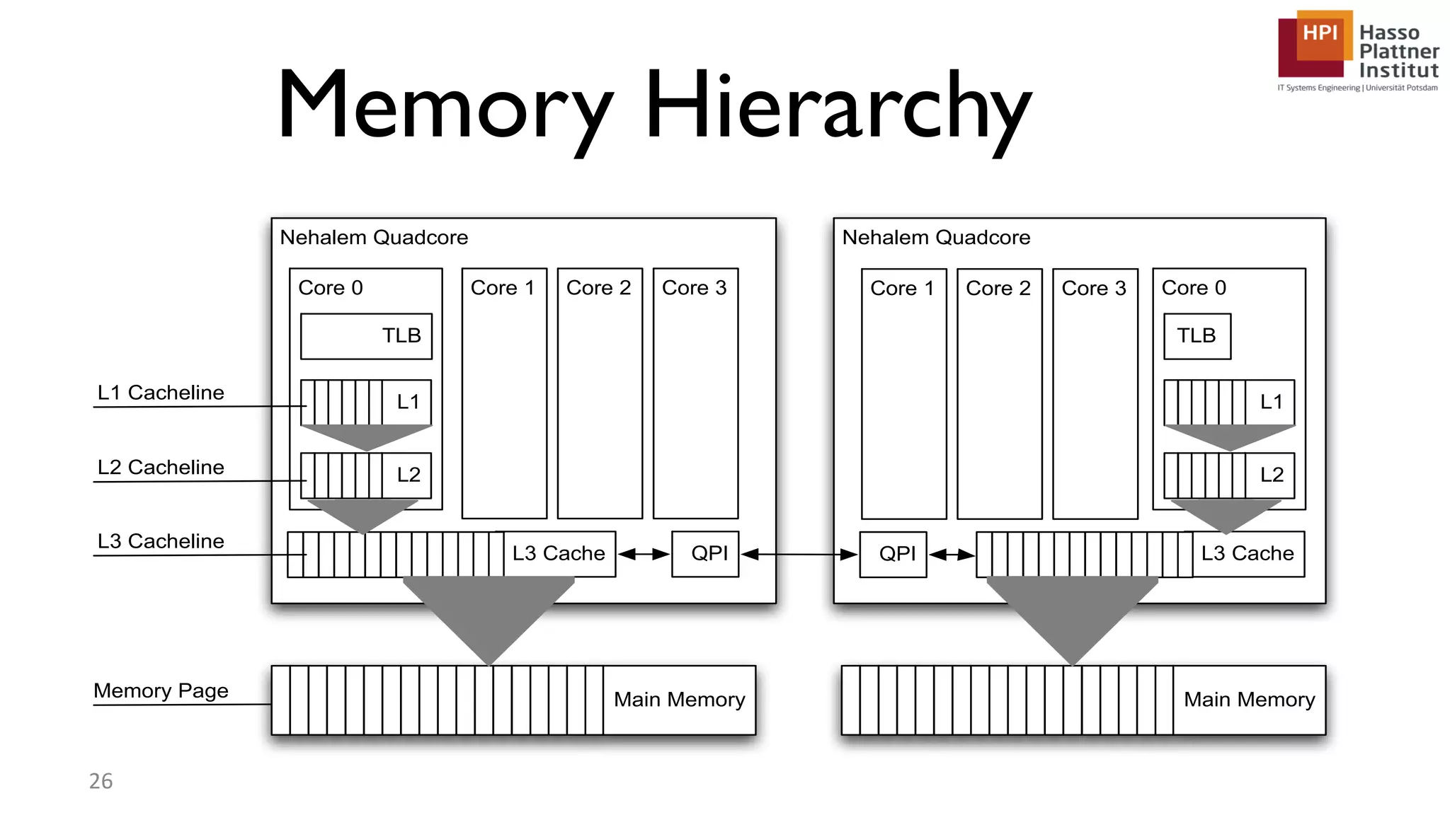
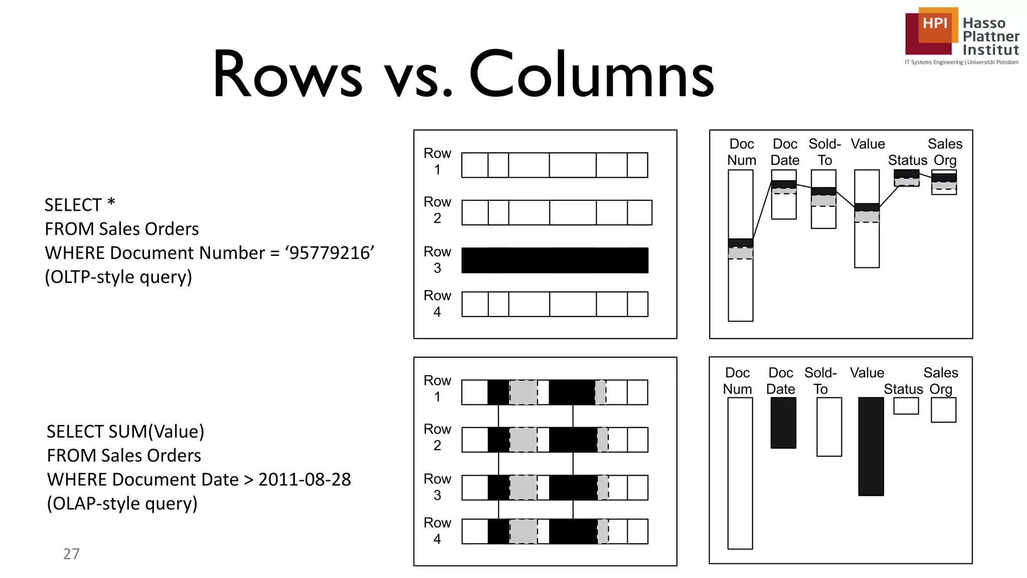
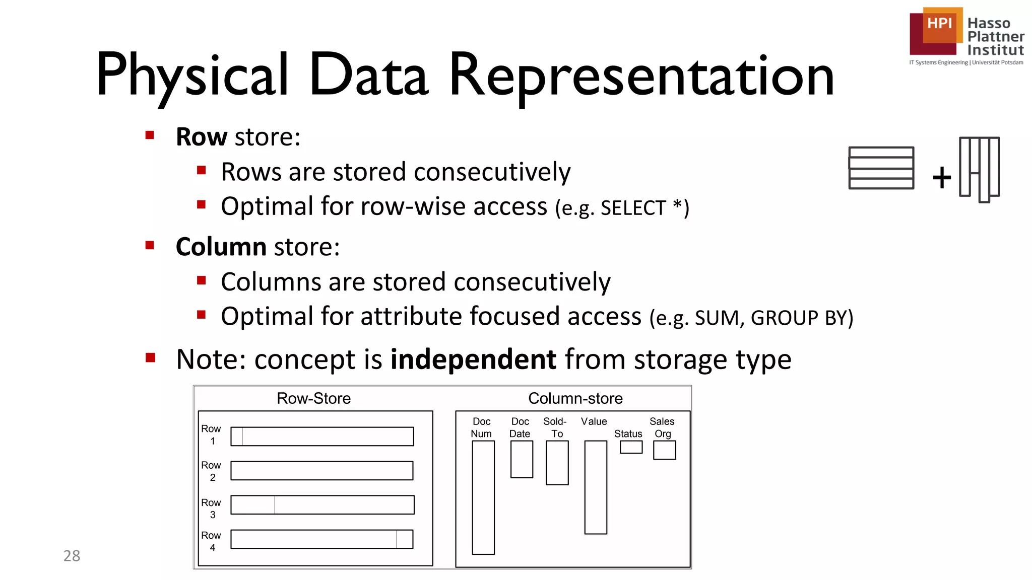
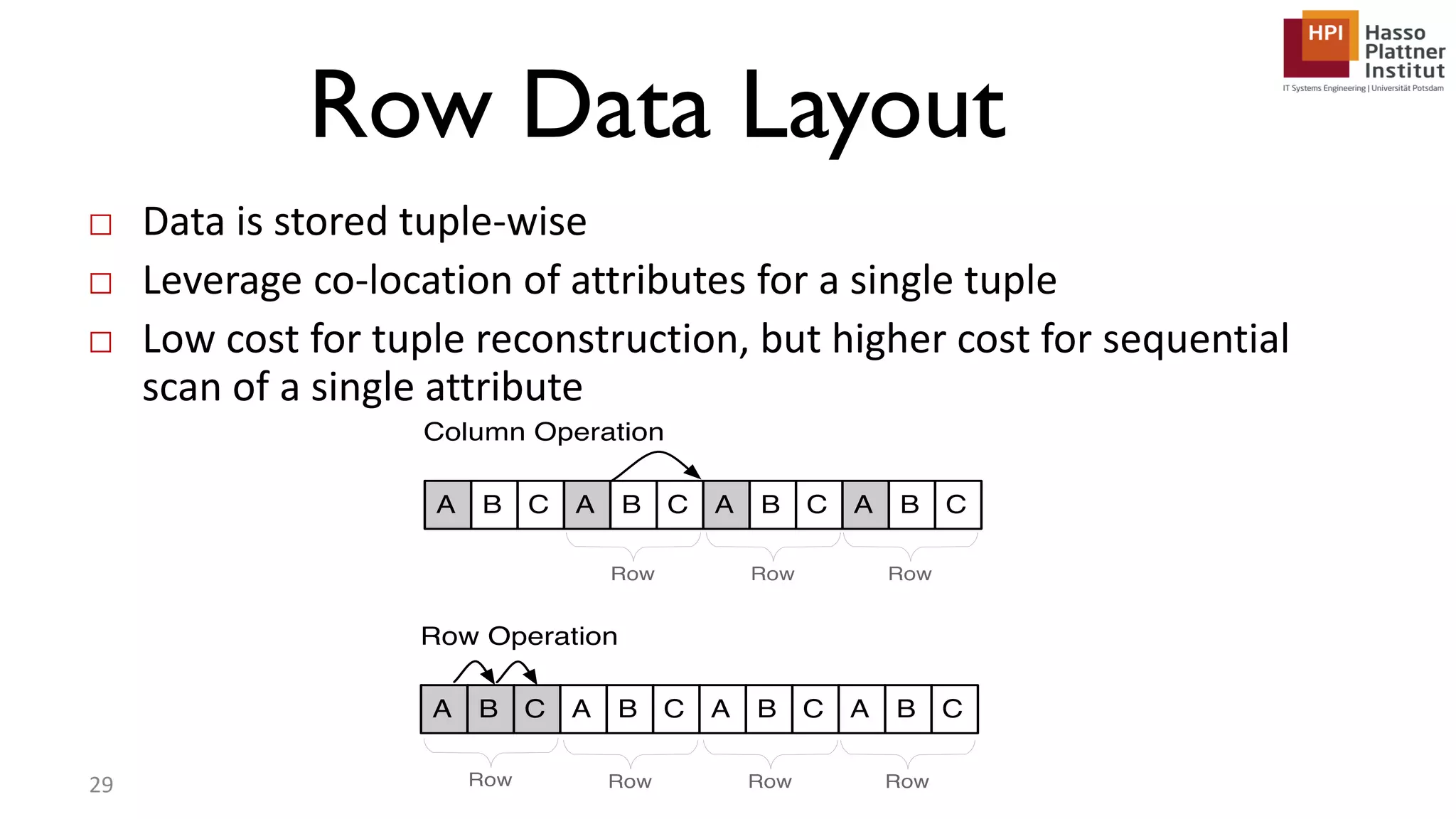
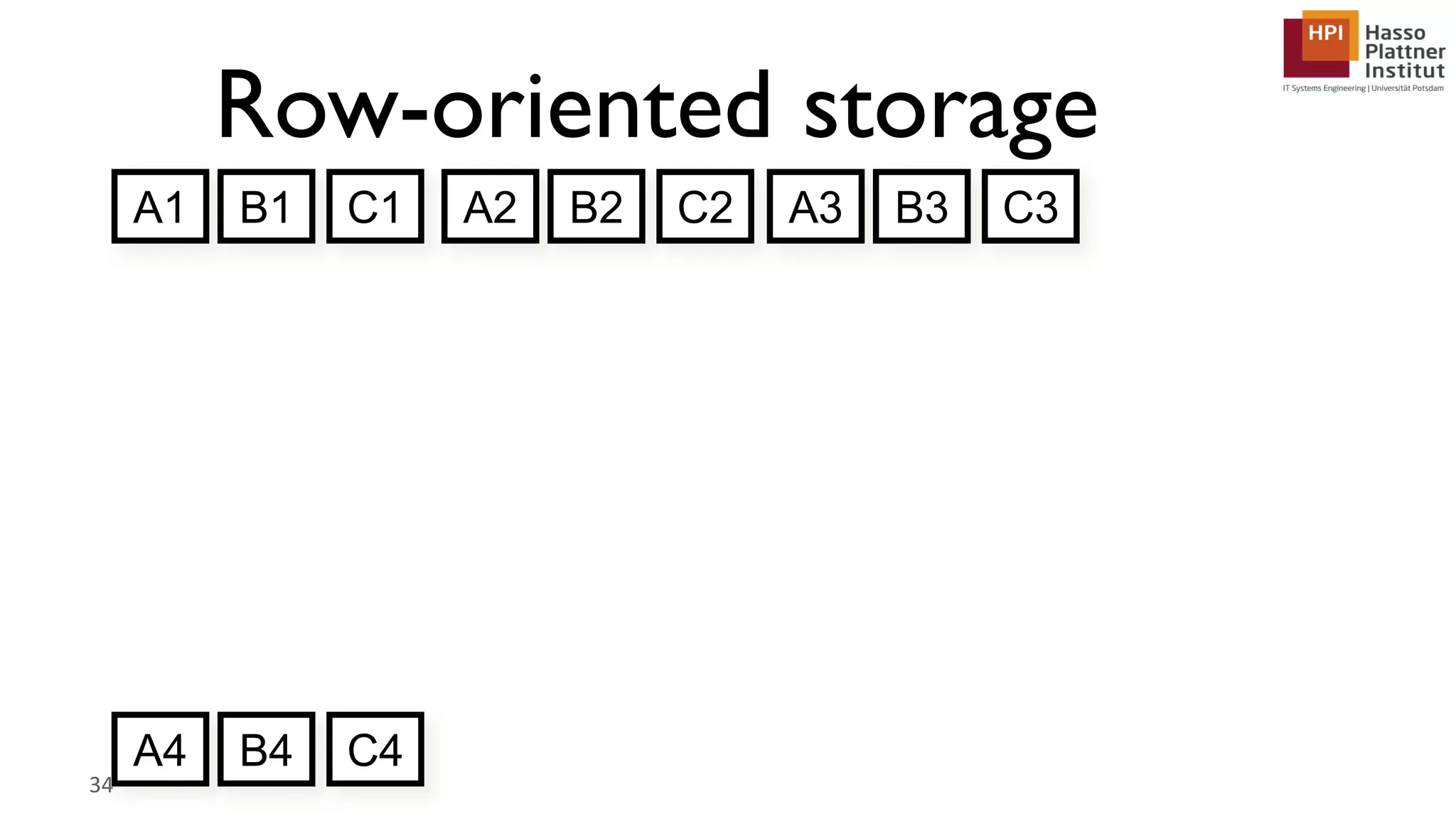
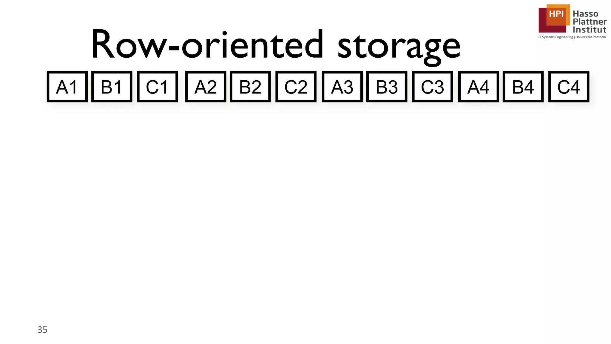
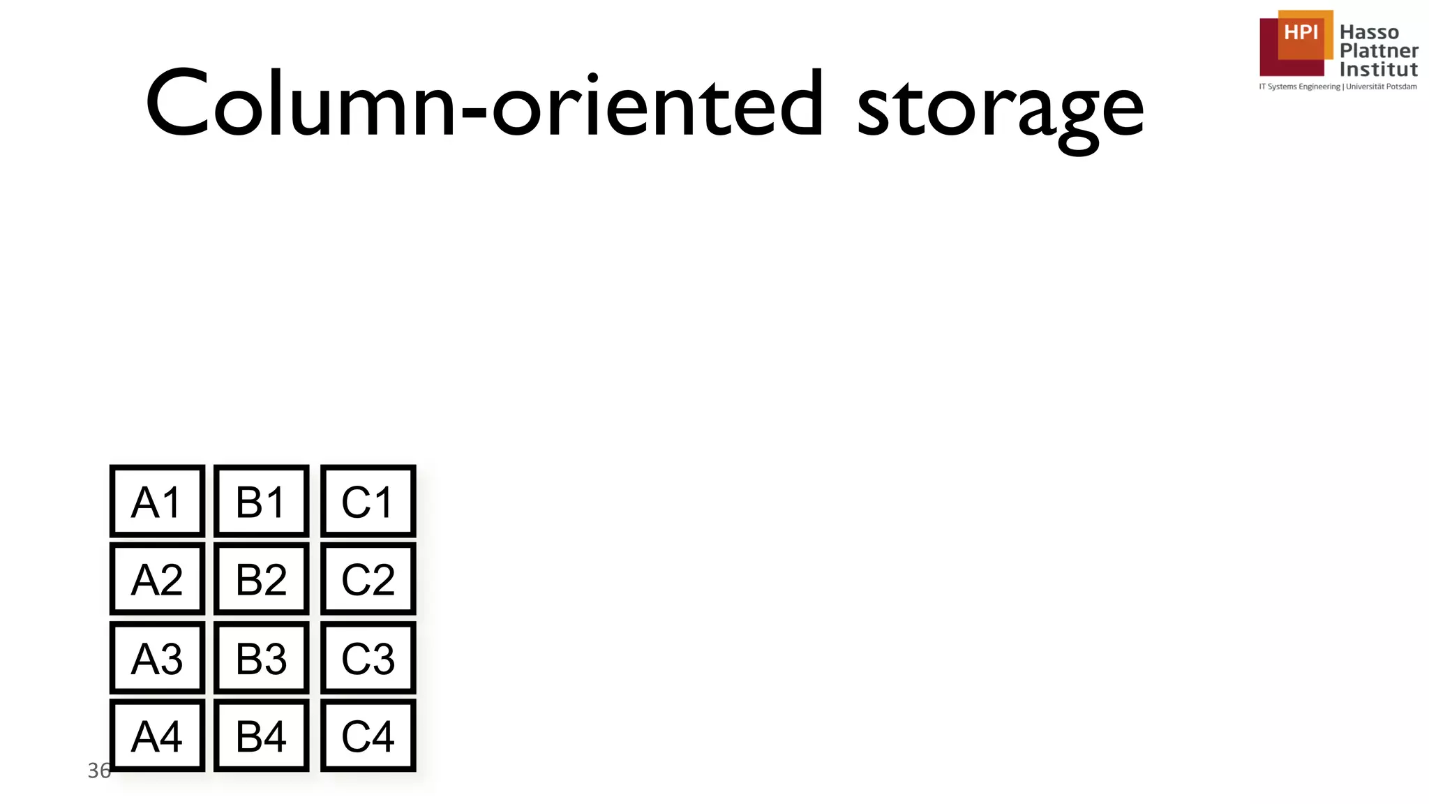
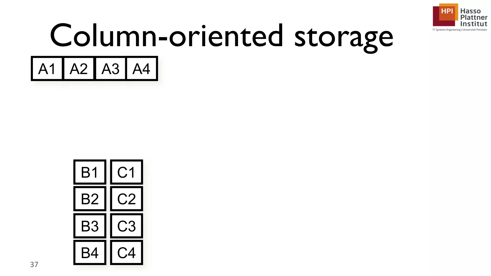
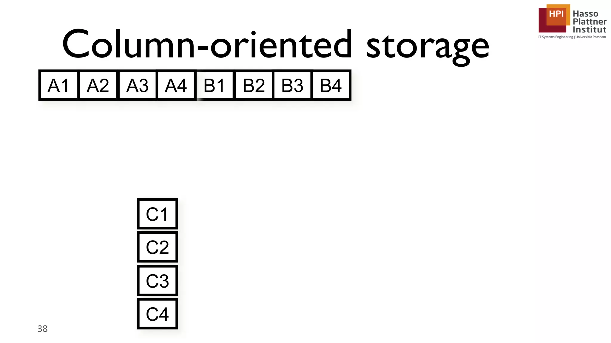
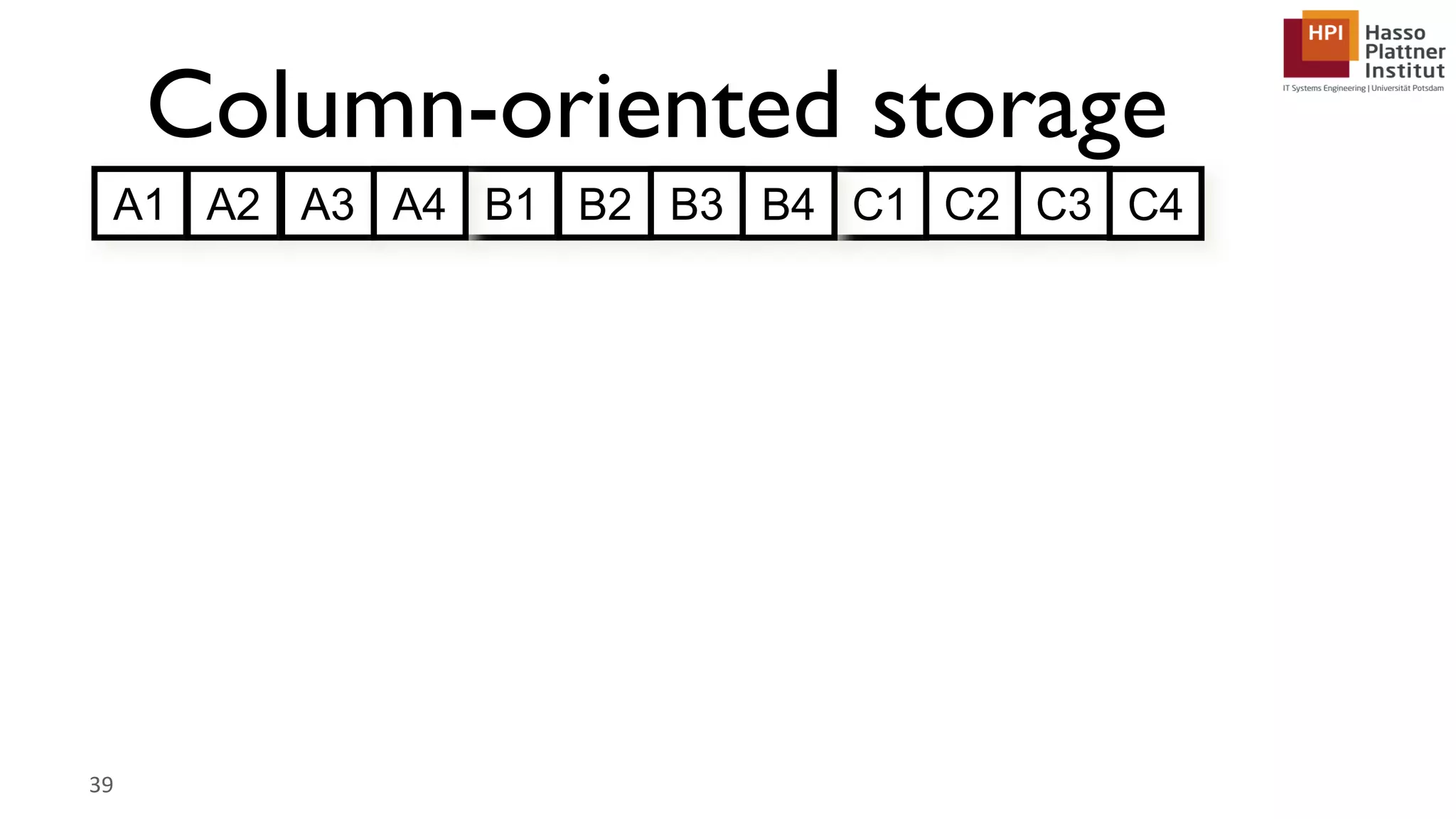
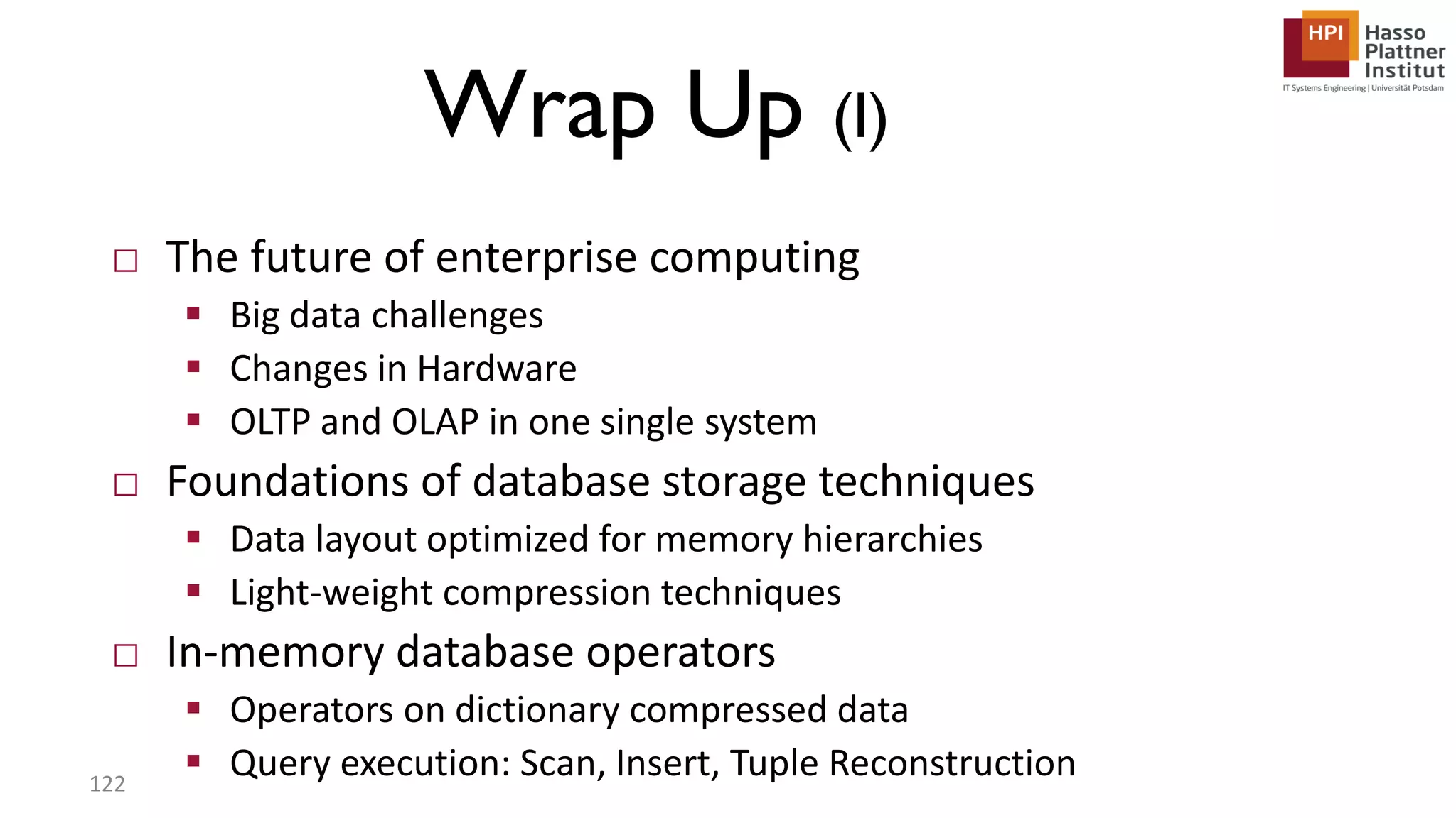
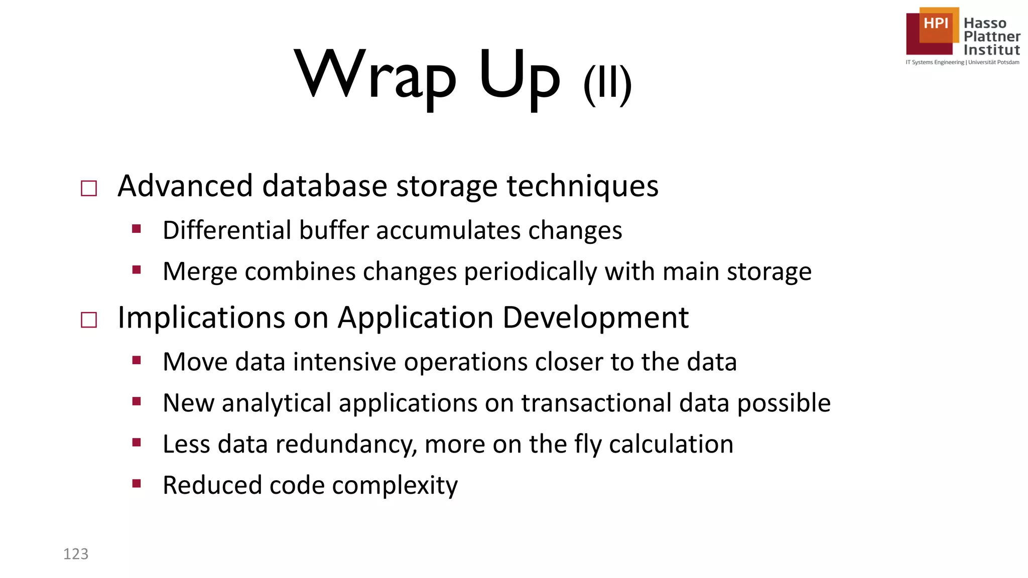
Sap technical deep dive in a column oriented in memory database

CD216: Technical Deep-Dive in a Column-Oriented In-Memory Database Dr. Jan Schaffner Research Group of Prof. Hasso Plattner Hasso Plattner Institute for Software Engineering University of Potsdam

Goals Deep technical understanding of a column-oriented, dictionary-encoded in-memory database and its application in enterprise computing 2

Chapters □ The status quo in enterprise computing □ Foundations of database storage techniques □ In-memory database operators □ Advanced database storage techniques □ Implications on Application Development 3

Learning Map of our Online Lecture @ openHPI.de Foundations for a New Enterprise Application Development Era Foundations of Database Storage Techniques The Future of Enterprise Computing Advanced Database Storage Tech- niques In-Memory Database Operators

Chapter 1: The Status Quo in Enterprise Computing

 Modern enterprise resource planning (ERP) systems are challenged by mixed workloads, including OLAP-style queries. For example:  OLTP-style: create sales order, invoice, accounting documents, display customer master data or sales order  OLAP-style: dunning, available-to-promise, cross selling, operational reporting (list open sales orders) Online Transaction Processing Online Analytical Processing OLTP vs. OLAP 6

Online Transaction Processing Online Analytical Processing OLTP vs. OLAP 7 But: Today’s data management systems are optimized either for daily transactional or analytical workloads storing their data along rows or columns

Drawbacks of the Separation  OLAP systems do not have the latest data  OLAP systems only have predefined subset of the data  Cost-intensive ETL processes have to sync both systems  Separation introduces data redundancy  Different data schemas introduce complexity for applications combining sources 8

EnterpriseWorkloads are Read Dominated 0 % 10 % 20 % 30 % 40 % 50 % 60 % 70 % 80 % 90 % 100% OLTP OLAP Workload 0 % 10 % 20 % 30 % 40 % 50 % 60 % 70 % 80 % 90 % 100% TPC-CWorkload Select Insert Modification Delete Write: Read: Lookup Table Scan Range Select Insert Modification Delete Write: Read:  Workload in enterprise applications constitutes of  Mainly read queries (OLTP 83%, OLAP 94%)  Many queries access large sets of data 9

Few Updates in OLTP Percentageofrowsupdated 10

Combine OLTP and OLAP data using modern hardware and database systems to create a single source of truth, enable real-time analytics and simplify applications and database structures. Vision 11

Additionally,  Extraction, transformation, and loading (ETL) processes  Pre-computed aggregates and materialized views become (almost) obsolete. Vision 12

 Many columns are not used even once  Many columns have a low cardinality of values  NULL values/default values are dominant  Sparse distribution facilitates high compression Standard enterprise software data is sparse and wide. Enterprise Data Characteristics 13

Sparse Tables 0% 10% 20% 30% 40% 50% 60% 70% 80% 1 - 32 33 - 1023 1024 - 100000000 13% 9 % 78% 24% 12% 64% Number of Distinct Values Inventory Management Financial Accounting %ofColumns 14

Sparse Tables 55% unused columns per company in average 40% unused columns across all analyzed companies 15

A Changes in Hardware… … give an opportunity to re-think the assumptions of yesterday because of what is possible today.  Main Memory becomes cheaper and larger ■ Multi-Core Architecture (96 cores per server) ■ Large main memories: 4TB /blade ■ One enterprise class server ~$50.000 ■ Parallel scaling across blades ■ 64-bit address space ■ 4TB in current servers ■ Cost-performance ratio rapidly declining ■ Memory hierarchies 17

In the Meantime Research has come up with…  Column-oriented data organization (the column store)  Sequential scans allow best bandwidth utilization between CPU cores and memory  Independence of tuples allows easy partitioning and therefore parallel processing  Lightweight Compression  Reducing data amount  Increasing processing speed through late materialization  And more, e.g., parallel scan/join/aggregation … several advances in software for processing data + 18

SanssouciDB: An In-Memory Database for Enterprise Applications Main Memory at Blade i Log SnapshotsPassive Data (History) Non-Volatile Memory RecoveryLogging Time travel Data aging Query Execution Metadata TA Manager Interface Services and Session Management Distribution Layer at Blade i Main Store Differential Store Active Data Merge Column Column Combined Column Column Column Combined Column Indexes Inverted Object Data Guide Main Memory at Server i Distribution Layer at Server i

SanssouciDB: An In-Memory Database for Enterprise Applications In-Memory Database (IMDB)  Data resides permanently in main memory  Main Memory is the primary “persistence”  Still: logging and recovery to/from flash  Main memory access is the new bottleneck  Cache-conscious algorithms/ data structures are crucial (locality is king)

Chapter 2: Foundations of Database Storage Techniques

Memory Basics (1) □ Memory in today’s computers has a linear address layout: addresses start at 0x0 and go to 0xFFFFFFFFFFFFFFFF for 64bit □ Each process has its own virtual address space □ Virtual memory allocated by the program can distribute over multiple physical memory locations □ Address translation is done in hardware by the CPU 24

Memory Basics (2) □ Memory layout is only linear □ Every higher-dimensional access (like two-dimensional database tables) is mapped to this linear band 25

Memory Hierarchy 26 Memory Page Nehalem Quadcore Core 0 Core 1 Core 2 Core 3 L3 Cache L2 L1 TLB Main Memory Main Memory QPI Nehalem Quadcore Core 0Core 1 Core 2 Core 3 L3 Cache L2 L1 TLB QPI L1 Cacheline L2 Cacheline L3 Cacheline

Rows vs. Columns 27 SELECT * FROM Sales Orders WHERE Document Number = ‘95779216’ (OLTP-style query) SELECT SUM(Value) FROM Sales Orders WHERE Document Date > 2011-08-28 (OLAP-style query) Row 4 Row 3 Row 2 Row 1 Row 4 Row 3 Row 2 Row 1 Doc Num Doc Date Sold- To Value Status Sales Org Doc Num Doc Date Sold- To Value Status Sales Org

Physical Data Representation  Row store:  Rows are stored consecutively  Optimal for row-wise access (e.g. SELECT *)  Column store:  Columns are stored consecutively  Optimal for attribute focused access (e.g. SUM, GROUP BY)  Note: concept is independent from storage type + 28 Doc Num Doc Date Sold- To Value Status Sales Org Row 4 Row 3 Row 2 Row 1 Row-Store Column-store

Row Data Layout □ Data is stored tuple-wise □ Leverage co-location of attributes for a single tuple □ Low cost for tuple reconstruction, but higher cost for sequential scan of a single attribute 29

Columnar Data Layout □ Data is stored attribute-wise □ Leverage sequential scan-speed in main memory for predicate evaluation □ Tuple reconstruction is more expensive 30

Row-oriented storage 31 A1 B1 C1 A2 B2 C2 A3 B3 C3 A4 B4 C4

Column-oriented storage 36 A1 B1 C1 A2 B2 C2 A3 B3 C3 A4 B4 C4

Column-oriented storage 37 B1 C1 B2 C2 B3 C3 B4 C4 A1 A2 A3 A4

Column-oriented storage 38 A1 B1 C1 A2 B2 C2 A3 B3 C3 A4 B4 C4

Column-oriented storage 39 A1 B1 C1A2 B2 C2A3 B3 C3A4 B4 C4

Motivation □ Main memory access is the new bottleneck □ Idea: Trade CPU time to compress and decompress data □ Compression reduces number of memory accesses □ Leads to less cache misses due to more information on a cache line □ Operation directly on compressed data possible □ Offsetting with bit-encoded fixed-length data types □ Based on limited value domain 41

Dictionary Encoding Example 8 billion humans □ Attributes  first name  last name  gender  country  city  birthday  200 byte □ Each attribute is stored dictionary encoded 42

Sample Data 43 rec ID fname lname gender city country birthday … … … … … … … 39 John Smith m Chicago USA 12.03.1964 40 Mary Brown f London UK 12.05.1964 41 Jane Doe f Palo Alto USA 23.04.1976 42 John Doe m Palo Alto USA 17.06.1952 43 Peter Schmidt m Potsdam GER 11.11.1975 … … … … … …

Dictionary Encoding a Column □ A column is split into a dictionary and an attribute vector □ Dictionary stores all distinct values with implicit value ID □ Attribute vector stores value IDs for all entries in the column □ Position is implicit, not stored explicitly □ Enables offsetting with fixed-length data types 44

Dictionary Encoding a Column 45 Rec ID fname … … 39 John 40 Mary 41 Jane 42 John 43 Peter … … Dictionary for “fname” Value ID Value … … 23 Jane 24 John … … 28 Mary 29 Peter Attribute Vector for “fname” position Value ID … … 39 24 40 28 41 23 42 24 43 29 … …

Sorted Dictionary □ Dictionary entries are sorted either by their numeric value or lexicographically  Dictionary lookup complexity: O(log(n)) instead of O(n) □ Dictionary entries can be compressed to reduce the amount of required storage □ Selection criteria with ranges are less expensive (order-preserving dictionary) 46

Data Size Examples 47 Column Cardi- nality Bits Needed Item Size Plain Size Size with Dictionary (Dictionary + Column) Compression Factor First name 5 million 23 bit 50 Byte 373 GB 238.4 MB + 21.4 GB ≈ 17 Last name 8 million 23 bit 50 Byte 373 GB 381.5 MB + 21.4 GB ≈ 17 Gender 2 1 bit 1 Byte 8 GB 2 bit + 1 GB ≈ 8 City 1 million 20 bit 50 Byte 373 GB 47.7 MB + 18.6 GB ≈ 20 Country 200 8 bit 47 Byte 350 GB 9.2 KB + 7.5 GB ≈ 47 Birthday 40,000 16 bit 2 Byte 15 GB 78.1 KB + 14.9 GB ≈ 1 Totals 200 Byte ≈ 1.6 TB ≈ 92 GB ≈ 17

Chapter 3: In-Memory Database Operators

Scan Performance (1) 8 billion humans  Attributes  First Name  Last Name  Gender  Country  City  Birthday  200 byte  Question: How many men/women?  Assumed scan speed: 2 MB/ms/core 49

Scan Performance (2) 50 Row Store – Layout  Table size = 8 billion tuples x 200 bytes per tuple  ~1.6 TB  Scan through all rows with 2 MB/ms/core  ~800 seconds with 1 core

Scan Performance (3) 51 Row Store – Full Table Scan  Table size = 8 billion tuples x 200 bytes per tuple  ~1.6 TB  Scan through all rows with 2 MB/ms/core  ~800 seconds with 1 core

Scan Performance (4) 52  8 billion cache accesses à 64 byte  ~512 GB  Read with 2 MB/ms/core  ~256 seconds with 1 core Row Store – Stride Access “Gender”

Scan Performance (5) 53 Column Store – Layout  Table size  Attribute vectors: ~91 GB  Dictionaries: ~700 MB  Total: ~92 GB  Compression factor: ~17

Scan Performance (6) 54 Column Store – Full Column Scan on “Gender”  Size of attribute vector “gender” = 8 billion tuples x 1 bit per tuple  ~1 GB  Scan through attribute vector with 2 MB/ms/core  ~0.5 seconds with 1 core

Scan Performance (7) 55 Column Store – Full Column Scan on “Birthday”  Size of attribute vector “birthday” = 8 billion tuples x 2 Byte per tuple  ~16 GB  Scan through column with 2 MB/ms/core  ~8 seconds with 1 core

Scan Performance – Summary 56  How many women, how many men? Column Store Row Store Full table scan Stride access Time in seconds 0.5 800 256 1,600x slower 512x slower

Parallel Aggregation 57  1.) n Aggregation Threads  1) each thread fetches a small part of the input relation  2) aggregate part and write results into a small hash-table  If the entries in a hash-table exceed a threshold, the hash-table is moved into a shared buffer  2.) m Merger Threads  3) each merge thread operates on a partition of the hash function values and writes its result into a private part hash- table  4) the final result is obtained by concatenating the part hash-tables

Tuple Reconstruction (1)  All attributes are stored consecutively  200 byte  4 cache accesses à 64 byte  256 byte  Read with 2 MB/ms/core  ~0.128 μs with 1 core Accessing a record in a row store 59 Table: world_population

Tuple Reconstruction (2)  All attributes are stored in separate columns  Implicit record IDs are used to reconstruct rows 60 Column store Table: world_population

Tuple Reconstruction (3)  1 cache access for each attribute  6 cache accesses à 64 byte  384 byte  Read with 2 MB/ms/core  ~0.192 μs with 1 core 61 Column store Table: world_population

SELECT Example SELECT fname, lname FROM world_population WHERE country="Italy" and gender="m" fname lname country gender Gianluigi Buffon Italy m Lena Gercke Germany f Mario Balotelli Italy m Manuel Neuer Germany m Lukas Podolski Germany m Klaas-Jan Huntelaar Netherlands m 63

Query Plan  Multiple plans possible to execute this query  Query Optimizer decides which is executed  Based on cost model, statistics and other parameters  Alternatives  Scan “country” and “gender”, positional AND  Scan over “country” and probe into “gender”  Indices might be used  Decision depends on data and query parameters like e.g. selectivity 64 SELECT fname, lname FROM world_population WHERE country="Italy" and gender="m"

Query Plan (i) Positional AND:  Predicates are evaluated and generate position lists  Intermediate position lists are logically combined  Final position list is used for materialization 65 π

Query Execution (i) Position 0 2 Position 0 2 3 4 5 Position 0 2 country = 3 ("Italy") gender = 1 ("m") AND Value ID Dictionary for “country” 0 Algeria 1 France 2 Germany 3 Italy 4 Netherlands … Value ID Dictionary for “gender” 0 f 1 m fname lname country gender Gianluigi Buffon 3 1 Lena Gercke 2 0 Mario Balotelli 3 1 Manuel Neuer 2 1 Lukas Podolski 2 1 Klaas-Jan Huntelaar 4 1 66

Query Plan (ii) Based on position list produced by first selection, gender column is probed. 67 π

Insert □ Insert is the dominant modification operation  Delete/Update can be modeled as Inserts as well (Insert-only approach) □ Inserting into a compressed in-memory persistence can be expensive  Updating sorted sequences (e.g. dictionaries) is a challenge  Inserting into columnar storages is generally more expensive than inserting into row storages 69

Insert Example rowID fname lname gender country city birthday 0 Martin Albrecht m GER Berlin 08-05-1955 1 Michael Berg m GER Berlin 03-05-1970 2 Hanna Schulze f GER Hamburg 04-04-1968 3 Anton Meyer m AUT Innsbruck 10-20-1992 4 Sophie Schulze f GER Potsdam 09-03-1977 ... ... ... ... ... ... ... world_population INSERT INTO world_population VALUES (Karen, Schulze, f, GER, Rostock, 11-15-2012) 70

INSERT (1) w/o new Dictionary entry fname lname gender country city birthday 0 Martin Albrecht m GER Berlin 08-05-1955 1 Michael Berg m GER Berlin 03-05-1970 2 Hanna Schulze f GER Hamburg 04-04-1968 3 Anton Meyer m AUT Innsbruck 10-20-1992 4 Sophie Schulze f GER Potsdam 09-03-1977 ... ... ... ... ... ... ... INSERT INTO world_population VALUES (Karen, Schulze, f, GER, Rostock, 11-15-2012) 0 0 1 1 2 3 3 2 4 3 0 Albrecht 1 Berg 2 Meyer 3 Schulze DAV Attribute Vector (AV) Dictionary (D) 71

0 Albrecht 1 Berg 2 Meyer 3 Schulze 1. Look-up on D  entry found INSERT INTO world_population VALUES (Karen, Schulze, f, GER, Rostock, 11-15-2012) Attribute Vector (AV) Dictionary (D) D fname lname gender country city birthday 0 Martin Albrecht m GER Berlin 08-05-1955 1 Michael Berg m GER Berlin 03-05-1970 2 Hanna Schulze f GER Hamburg 04-04-1968 3 Anton Meyer m AUT Innsbruck 10-20-1992 4 Sophie Schulze f GER Potsdam 09-03-1977 ... ... ... ... ... ... ... AV 0 0 1 1 2 3 3 2 4 3 INSERT (1) w/o new Dictionary entry 72

0 0 1 1 2 3 3 2 4 3 5 3 1. Look-up on D  entry found 2. Append ValueID to AV INSERT INTO world_population VALUES (Karen, Schulze, f, GER, Rostock, 11-15-2012) Attribute Vector (AV) Dictionary (D) fname lname gender country city birthday 0 Martin Albrecht m GER Berlin 08-05-1955 1 Michael Berg m GER Berlin 03-05-1970 2 Hanna Schulze f GER Hamburg 04-04-1968 3 Anton Meyer m AUT Innsbruck 10-20-1992 4 Sophie Schulze f GER Potsdam 09-03-1977 5 Schulze ... ... ... ... ... ... ... 0 Albrecht 1 Berg 2 Meyer 3 Schulze INSERT (1) w/o new Dictionary entry 73 DAV

INSERT (2) with new Dictionary Entry I/II fname lname gender country city birthday 0 Martin Albrecht m GER Berlin 08-05-1955 1 Michael Berg m GER Berlin 03-05-1970 2 Hanna Schulze f GER Hamburg 04-04-1968 3 Anton Meyer m AUT Innsbruck 10-20-1992 4 Sophie Schulze f GER Potsdam 09-03-1977 5 Schulze ... ... ... ... ... ... ... INSERT INTO world_population VALUES (Karen, Schulze, f, GER, Rostock, 11-15-2012) 0 0 1 0 2 1 3 2 4 3 0 Berlin 1 Hamburg 2 Innsbruck 3 Potsdam Attribute Vector (AV) Dictionary (D) 74 DAV

1. Look-up on D  no entry found INSERT INTO world_population VALUES (Karen, Schulze, f, GER, Rostock, 11-15-2012) 0 0 1 0 2 1 3 2 4 3 0 Berlin 1 Hamburg 2 Innsbruck 3 Potsdam fname lname gender country city birthday 0 Martin Albrecht m GER Berlin 08-05-1955 1 Michael Berg m GER Berlin 03-05-1970 2 Hanna Schulze f GER Hamburg 04-04-1968 3 Anton Meyer m AUT Innsbruck 10-20-1992 4 Sophie Schulze f GER Potsdam 09-03-1977 5 Schulze ... ... ... ... ... ... ... Attribute Vector (AV) Dictionary (D) INSERT (2) with new Dictionary Entry I/II 75 DAV

1. Look-up on D  no entry found 2. Append new value to D (no re-sorting necessary) INSERT INTO world_population VALUES (Karen, Schulze, f, GER, Rostock, 11-15-2012) 0 Berlin 1 Hamburg 2 Innsbruck 3 Potsdam 4 Rostock fname lname gender country city birthday 0 Martin Albrecht m GER Berlin 08-05-1955 1 Michael Berg m GER Berlin 03-05-1970 2 Hanna Schulze f GER Hamburg 04-04-1968 3 Anton Meyer m AUT Innsbruck 10-20-1992 4 Sophie Schulze f GER Potsdam 09-03-1977 5 Schulze ... ... ... ... ... ... ... Attribute Vector (AV) Dictionary (D) 0 0 1 0 2 1 3 2 4 3 INSERT (2) with new Dictionary Entry I/II 76 DAV

1. Look-up on D  no entry found 2. Append new value to D (no re-sorting necessary) 3. Append ValueID to AV INSERT INTO world_population VALUES (Karen, Schulze, f, GER, Rostock, 11-15-2012) fname lname gender country city birthday 0 Martin Albrecht m GER Berlin 08-05-1955 1 Michael Berg m GER Berlin 03-05-1970 2 Hanna Schulze f GER Hamburg 04-04-1968 3 Anton Meyer m AUT Innsbruck 10-20-1992 4 Sophie Schulze f GER Potsdam 09-03-1977 5 Schulze Rostock ... ... ... ... ... ... ... Attribute Vector (AV) Dictionary (D) 0 0 1 0 2 1 3 2 4 3 5 4 0 Berlin 1 Hamburg 2 Innsbruck 3 Potsdam 4 Rostock INSERT (2) with new Dictionary Entry I/II 77 DAV

0 Anton 1 Hanna 2 Martin 3 Michael 4 Sophie fname lname gender country city birthday 0 Martin Albrecht m GER Berlin 08-05-1955 1 Michael Berg m GER Berlin 03-05-1970 2 Hanna Schulze f GER Hamburg 04-04-1968 3 Anton Meyer m AUT Innsbruck 10-20-1992 4 Sophie Schulze f GER Potsdam 09-03-1977 5 Schulze Rostock ... ... ... ... ... ... ... INSERT INTO world_population VALUES (Karen, Schulze, f, GER, Rostock, 11-15-2012) 0 2 1 3 2 1 3 0 4 4 Attribute Vector (AV) Dictionary (D) INSERT (2) with new Dictionary Entry I/II 78 DAV

1. Look-up on D  no entry found INSERT INTO world_population VALUES (Karen, Schulze, f, GER, Rostock, 11-15-2012) fname lname gender country city birthday 0 Martin Albrecht m GER Berlin 08-05-1955 1 Michael Berg m GER Berlin 03-05-1970 2 Hanna Schulze f GER Hamburg 04-04-1968 3 Anton Meyer m AUT Innsbruck 10-20-1992 4 Sophie Schulze f GER Potsdam 09-03-1977 5 Schulze Rostock ... ... ... ... ... ... ... Attribute Vector (AV) Dictionary (D) 0 Anton 1 Hanna 2 Martin 3 Michael 4 Sophie 0 2 1 3 2 1 3 0 4 4 INSERT (2) with new Dictionary Entry II/II 79 DAV

1. Look-up on D  no entry found 2. Insert new value to D INSERT INTO world_population VALUES (Karen, Schulze, f, GER, Rostock, 11-15-2012) fname lname gender country city birthday 0 Martin Albrecht m GER Berlin 08-05-1955 1 Michael Berg m GER Berlin 03-05-1970 2 Hanna Schulze f GER Hamburg 04-04-1968 3 Anton Meyer m AUT Innsbruck 10-20-1992 4 Sophie Schulze f GER Potsdam 09-03-1977 5 Schulze Rostock ... ... ... ... ... ... ... Attribute Vector (AV) Dictionary (D) 0 Anton 1 Hanna 2 Karen 3 Martin 4 Michael 5 Sophie 0 2 1 3 2 1 3 0 4 4 INSERT (2) with new Dictionary Entry II/II 80 DAV

1. Look-up on D  no entry found 2. Insert new value to D INSERT INTO world_population VALUES (Karen, Schulze, f, GER, Rostock, 11-15-2012) fname lname gender country city birthday 0 Martin Albrecht m GER Berlin 08-05-1955 1 Michael Berg m GER Berlin 03-05-1970 2 Hanna Schulze f GER Hamburg 04-04-1968 3 Anton Meyer m AUT Innsbruck 10-20-1992 4 Sophie Schulze f GER Potsdam 09-03-1977 5 Schulze Rostock ... ... ... ... ... ... ... Attribute Vector (AV) Dictionary (D) 0 Anton 1 Hanna 2 Martin 3 Michael 4 Sophie 0 2 1 3 2 1 3 0 4 4 0 Anton 1 Hanna 2 Karen 3 Martin 4 Michael 5 Sophie D (new) INSERT (2) with new Dictionary Entry II/II 81 D (old)AV

1. Look-up on D  no entry found 2. Insert new value to D 3. Change ValueIDs in AV INSERT INTO world_population VALUES (Karen, Schulze, f, GER, Rostock, 11-15-2012) fname lname gender country city birthday 0 Martin Albrecht m GER Berlin 08-05-1955 1 Michael Berg m GER Berlin 03-05-1970 2 Hanna Schulze f GER Hamburg 04-04-1968 3 Anton Meyer m AUT Innsbruck 10-20-1992 4 Sophie Schulze f GER Potsdam 09-03-1977 5 Schulze Rostock ... ... ... ... ... ... ... Attribute Vector (AV) Dictionary (D) AV (old) 0 Anton 1 Hanna 2 Karen 3 Martin 4 Michael 5 Sophie D (new)AV (new) 0 3 1 4 2 1 3 0 4 5 0 2 1 3 2 1 3 0 4 4 INSERT (2) with new Dictionary Entry II/II 82

1. Look-up on D  no entry found 2. Insert new value to D 3. Change ValueIDs in AV 4. Append new ValueID to AV INSERT INTO world_population VALUES (Karen, Schulze, f, GER, Rostock, 11-15-2012) fname lname gender country city birthday 0 Martin Albrecht m GER Berlin 08-05-1955 1 Michael Berg m GER Berlin 03-05-1970 2 Hanna Schulze f GER Hamburg 04-04-1968 3 Anton Meyer m AUT Innsbruck 10-20-1992 4 Sophie Schulze f GER Potsdam 09-03-1977 5 Karen Schulze Rostock ... ... ... ... ... ... ... Attribute Vector (AV) Dictionary (D) 0 Anton 1 Hanna 2 Karen 3 Martin 4 Michael 5 Sophie 0 3 1 4 2 1 3 0 4 5 5 2 INSERT (2) with new Dictionary Entry II/II 83 Changed Value IDs DAV

Result rowID fname lname gender country city birthday 0 Martin Albrecht m GER Berlin 08-05-1955 1 Michael Berg m GER Berlin 03-05-1970 2 Hanna Schulze f GER Hamburg 04-04-1968 3 Anton Meyer m AUT Innsbruck 10-20-1992 4 Ulrike Schulze f GER Potsdam 09-03-1977 5 Karen Schulze f GER Rostock 11-15-2012 world_population INSERT INTO world_population VALUES (Karen, Schulze, f, GER, Rostock, 11-15-2012) 84

Chapter 4: Advanced Database StorageTechniques

Motivation □ Inserting new tuples directly into a compressed structure can be expensive  Especially when using sorted structures  New values can require reorganizing the dictionary  Number of bits required to encode all dictionary values can change, attribute vector has to be reorganized 87

Differential Buffer  New values are written to a dedicated differential buffer (Delta)  Cache Sensitive B+ Tree (CSB+) used for fast search on Delta DictionaryAttribute Vector fname … (compressed) Main Store Dictionary Attribute Vector CSB+ fname … Differential Buffer/ Delta WriteRead world_population 0 0 1 1 2 1 3 3 4 2 5 1 0 Anton 1 Hanna 2 Michael 3 Sophie 0 Angela 1 Klaus 2 Andre 0 0 1 1 2 1 3 2 8 Billion entries up to 50,000 entries 88

Differential Buffer □ Inserts of new values are fast, because dictionary and attribute vector do not need to be resorted □ Range selects on differential buffer are expensive  Unsorted dictionary allows no direct comparison of value IDs  Scans with range selection need to lookup values in dictionary for comparisons □ Differential Buffer requires more memory:  Attribute vector not bit-compressed  Additional CSB+ Tree for dictionary 89

recId fname lname gender country city birthday 0 Martin Albrecht m GER Berlin 08-05-1955 1 Michael Berg m GER Berlin 03-05-1970 2 Hanna Schulze f GER Hamburg 04-04-1968 3 Anton Meyer m AUT Innsbruck 10-20-1992 ... ... ... ... ... ... ... 8 * 109 Zacharias Perdopolus m GRE Athen 03-12-1979 Differential Buffer Main Store Tuple Lifetime Main Table: world_population Michael moves from Berlin to Potsdam UPDATE "world_population" SET city="Potsdam" WHERE fname="Michael" AND lname="Berg" 90

recId fname lname gender country city birthday 0 Martin Albrecht m GER Berlin 08-05-1955 1 Michael Berg m GER Berlin 03-05-1970 2 Hanna Schulze f GER Hamburg 04-04-1968 3 Anton Meyer m AUT Innsbruck 10-20-1992 ... ... ... ... ... ... ... 8 * 109 Zacharias Perdopolus m GRE Athen 03-12-1979 Differential Buffer Main Store Tuple Lifetime UPDATE "world_population" SET city="Potsdam" WHERE fname="Michael" AND lname="Berg" 91 Main Table: world_population Michael moves from Berlin to Potsdam

recId fname lname gender country city birthday 0 Martin Albrecht m GER Berlin 08-05-1955 1 Michael Berg m GER Berlin 03-05-1970 2 Hanna Schulze f GER Hamburg 04-04-1968 3 Anton Meyer m AUT Innsbruck 10-20-1992 ... ... ... ... ... ... ... 8 * 109 Zacharias Perdopolus m GRE Athen 03-12-1979 Tuple Lifetime UPDATE "world_population" SET city="Potsdam" WHERE fname="Michael" AND lname="Berg" 0 Michael Berg m GER Potsdam 03-05-1970 92 Differential Buffer Main Store Main Table: world_population Michael moves from Berlin to Potsdam

Tuple Lifetime □ Tuples are now available in Main Store and Differential Buffer □ Tuples of a table are marked by a validity vector to reduce the required amount of reorganization steps  Additional attribute vector for validity  1 bit required per database tuple □ Invalidated tuples stay in the database table, until the next reorganization takes place □ Query results  Main and delta have to be queried  Results are filtered using the validity vector93

recId fname lname gender country city birthday valid 0 Martin Albrecht m GER Berlin 08-05-1955 1 1 Michael Berg m GER Berlin 03-05-1970 0 2 Hanna Schulze f GER Hamburg 04-04-1968 1 3 Anton Meyer m AUT Innsbruck 10-20-1992 1 ... ... ... ... ... ... ... 8 * 109 Zacharias Perdopolus m GRE Athen 03-12-1979 1 Tuple Lifetime UPDATE "world_population" SET city="Potsdam" WHERE fname="Michael" AND lname="Berg" 0 Michael Berg m GER Potsdam 03-05-1970 1 Differential Buffer Main Store 94 Main Table: world_population Michael moves from Berlin to Potsdam

Handling Write Operations  All Write operations (INSERT, UPDATE) are stored within a differential buffer (delta) first  Read-operations on differential buffer are more expensive than on main store □ Differential buffer is merged periodically with the main store  To avoid performance degradation based on large delta  Merge is performed asynchronously 96

Merge Overview I/II  The merge process is triggered for single tables  Is triggered by:  Amount of tuples in buffer  Cost model to  Schedule  Take query cost into account  Manually 97

Merge Overview II/II  Working on data copies allows asynchronous merge  Very limited interruption due to short lock  At least twice the memory of the table needed! 98 Prepare Attribute Merge Commit

Chapter 5: Implications on Application Development

How does it all come together? 1. Mixed Workload combining OLTP and analytic-style queries ■ Column-Stores are best suited for analytic-style queries ■ In-memory databases enable fast tuple re-construction ■ In-memory column store allows aggregation on-the-fly 2. Sparse enterprise data ■ Lightweight compression schemes are optimal ■ Increases query execution ■ Improves feasibility of in-memory databases 100

How does it all come together? 3. Mostly read workload ■ Read-optimized stores provide best throughput ■ i.e. compressed in-memory column-store ■ Write-optimized store as delta partition to handle data changes is sufficient 101 Changed Hardware Advances in data processing (software) Complex Enterprise Applications Our focus

An In-Memory Database for Enterprise Applications □ In-Memory Database (IMDB)  Data resides permanently in main memory  Main Memory is the primary “persistence”  Still: logging and recovery from/to flash  Main memory access is the new bottleneck  Cache-conscious algorithms/ data structures are crucial (locality is king) 102 Main Memory at Blade i Log SnapshotsPassive Data (History) Non-Volatile Memory RecoveryLogging Time travel Data aging Query Execution Metadata TA Manager Interface Services and Session Management Distribution Layer at Blade i Main Store Differential Store Active Data Merge Column Column Combined Column Column Column Combined Column Indexes Inverted Object Data Guide

Simplified Application Development Traditional Column-oriented Application cache Database cache Prebuilt aggregates Raw data 103  Fewer caches necessary  No redundant data (OLAP/OLTP, LiveCache)  No maintenance of materialized views or aggregates  Minimal index maintenance

Examples for Implications on Enterprise Applications

SAP ERP Financials on In-Memory Technology In-memory column database for an ERP system □ Combined workload (parallel OLTP/OLAP queries) □ Leverage in-memory capabilities to  Reduce amount of data  Aggregate on-the-fly  Run analytic-style queries (to replace materialized views)  Execute stored procedures 105

SAP ERP Financials on In-Memory Technology In-memory column database for an ERP system □ Use Case: SAP ERP Financials solution  Post and change documents  Display open items  Run dunning job  Analytical queries, such as balance sheet 106

Current Financials Solutions 107

Only base tables, algorithms, and some indices The Target Financials Solution 108

Feasibility of Financials on In- MemoryTechnology in 2009 □ Modifications on SAP Financials  Removed secondary indices, sum tables and pre-calculated and materialized tables  Reduce code complexity and simplify locks  Insert Only to enable history (change document replacement)  Added stored procedures with business functionality 109

Feasibility of Financials on In- MemoryTechnology in 2009 □ European division of a retailer  ERP 2005 ECC 6.0 EhP3  5.5 TB system database size  Financials:  23 million headers / 1.5 GB in main memory  252 million items / 50 GB in main memory (including inverted indices for join attributes and insert only extension) 110

BKPF accounting documents BSEG sum tables secondary indices dunning data change documents CDHDR CDPOS MHNK MHNDBSAD BSAK BSAS BSID BSIK BSIS LFC1 KNC1 GLT0 111 In-Memory Financials on SAP ERP

BKPF accounting documents BSEG In-Memory Financials on SAP ERP 112

Classic Row-Store (w/o compr.) IMDB BKPF 8.7 GB 1.5 GB BSEG 255 GB 50 GB Secondary Indices 255 GB - Sum Tables 0.55 GB - Complete 519.25 GB 51.5 GB 263.7 GB 51.5 GB Reduction by a Factor 10 113

Booking an accounting document □ Insert into BKPF and BSEG only □ Lack of updates reduces locks 114

Dunning Run □ Dunning run determines all open and due invoices □ Customer defined queries on 250M records □ Current system: 20 min □ New logic: 1.5 sec  In-memory column store  Parallelized stored procedures  Simplified Financials 115

Bring Application Logic Closer to the Storage Layer □ Select accounts to be dunned, for each:  Select open account items from BSID, for each:  Calculate due date  Select dunning procedure, level and area  Create MHNK entries □ Create and write dunning item tables 116

□ Select accounts to be dunned, for each:  Select open account items from BSID, for each:  Calculate due date  Select dunning procedure, level and area  Create MHNK entries □ Create and write dunning item tables 1 SELECT 10000 SELECTs 10000 SELECTs 31000 Entries 117 Bring Application Logic Closer to the Storage Layer

Bring Application Logic Closer to the Storage Layer □ Select accounts to be dunned, for each:  Select open account items from BSID, for each:  Calculate due date  Select dunning procedure, level and area  Create MHNK entries □ Create and write dunning item tables 118 1 SELECT 10000 SELECTs 10000 SELECTs 31000 Entries One single stored procedure executed within IMDB

Bring Application Logic Closer to the Storage Layer □ Select accounts to be dunned, for each:  Select open account items from BSID, for each:  Calculate due date  Select dunning procedure, level and area  Create MHNK entries □ Create and write dunning item tables Calculated on- the-fly 119 One single stored procedure executed within IMDB

Wrap Up (I) □ The future of enterprise computing  Big data challenges  Changes in Hardware  OLTP and OLAP in one single system □ Foundations of database storage techniques  Data layout optimized for memory hierarchies  Light-weight compression techniques □ In-memory database operators  Operators on dictionary compressed data  Query execution: Scan, Insert, Tuple Reconstruction122

Wrap Up (II) □ Advanced database storage techniques  Differential buffer accumulates changes  Merge combines changes periodically with main storage □ Implications on Application Development  Move data intensive operations closer to the data  New analytical applications on transactional data possible  Less data redundancy, more on the fly calculation  Reduced code complexity 123

Cooperation with Industry Partners □ Real use cases from industry partners □ Benefit for partners  Cutting edge soft- and hardware technologies  IT students work on new ideas from scratch or in addition to existing solutions □ Long track of success with partners  Multiple global enterprises from retail, engineering and other sectors  Improvement of modern ERP and analytical systems  New applications for mobile use cases 124

References □ A Course in In-Memory Data Management, H. Plattner http://epic.hpi.uni-potsdam.de/Home/InMemoryBook □ Publications of our Research Group:  Papers about the inner-workings of in-mmeory databases  http://epic.hpi.uni-potsdam.de/Home/Publications 125

ThankYou! CD216: Technical Deep-Dive in a Column-Oriented In-Memory Database Dr. Jan Schaffner Research Group of Prof. Hasso Plattner Hasso Plattner Institute for Software Engineering University of Potsdam

Available-to-Promise Check □ Can I get enough quantities of a requested product on a desired delivery date? □ Goal: Analyze and validate the potential of in-memory and highly parallel data processing for Available-to-Promise (ATP) □ Challenges  Dynamic aggregation  Instant rescheduling in minutes vs. nightly batch runs  Real-time and historical analytics □ Outcome  Real-time ATP checks without materialized views  Ad-hoc rescheduling  No materialized aggregates 130

In-Memory Available-to- Promise 131

Demand Planning □ Flexible analysis of demand planning data □ Zooming to choose granularity □ Filter by certain products or customers □ Browse through time spans □ Combination of location-based geo data with planning data in an in-memory database □ External factors such as the temperature, or the level of cloudiness can be overlaid to incorporate them in planning decisions 132

GORFID □ HANA for Streaming Data Processing □ Use Case: In-Memory RFID Data Management □ Evaluation of SAP OER □ Prototypical implementation of:  RFID Read Event Repository on HANA  Discovery Service on HANA (10 billion data records with ~3 seconds response time)  Front ends for iPhone & iPad □ Key Findings:  HANA is suited for streaming data (using bulk inserts)  Analytics on streaming data is now possible 133

GORFID:“Near Real-Time” as a Concept Bulk load every 2-3 seconds: > 50,000 inserts/s 134

Sap technical deep dive in a column oriented in memory database

More Related Content

What's hot

Viewers also liked

Similar to Sap technical deep dive in a column oriented in memory database

Recently uploaded

Sap technical deep dive in a column oriented in memory database