Randomized Algorithm- Advanced Algorithm

Presented To: Nusrat Jahan Id: B-150305002 Fahima Hossain Id: B-150305036 2 Dr. Md. Manowarul Islam Associate Professor Dept. of Computer Science & Engineering, Jagannath University, Dhaka Presented By:

Outline  Deterministic VS Non-Deterministic  Deterministic Algorithm  Randomized Algorithms  Types of Randomized Algorithms  Las Vegas  Monte Carlo  Las Vegas  Quick Sort  Smallest Enclosing Circle  Monto Carlo  Minimum Cut  Primality Testing  Smallest Enclosing Disk  Minimum Spanning Tree  Michael's Algorithms 3

Determinictic vs Non- Deterministic 1

Deterministic vs Non-Deterministic  Deterministic Algorithm: • In deterministic algorithm, for a given particular input, the computer will always produce the same output going through the same states. • Can solve the problem in polynomial time. • Can determine what is the next step.  Non-Deterministic Algorithm: • In non-deterministic algorithm, for the same input, the compiler may produce different output in different runs. • Can’t solve the problem in polynomial time. • Can’t determine what is the next step. 5

Deterministic Algorithm 6 Goal of Deterministic Algorithm The solution produced by the algorithm is correct. The number of computational steps is same for different runs of the algorithm with the same input.

Deterministic Algorithm 7 Problem in Deterministic Algorithm  Given a computational problem – • It may be difficult to formulate an algorithm with good running time, or • The exploitation of running time of an algorithm for that problem with the number of inputs. Efficient heuristics, Approximation algorithms, Randomized algorithms  Remedies

Randomized Algorithm 9 What is a Randomized Algorithm? • An algorithm that uses random numbers to decide what to do next anywhere in its logic is called Randomized Algorithm. • A randomized algorithm is an algorithm that employees a degree of randomness as a part of its logic. • A randomized algorithm is one that makes random choices during its execution.

“  To overcome the computation problem of exploitation of running time of a deterministic algorithm, randomized algorithm is used.  Randomized algorithm uses uniform random bits also called as pseudo random number as an input to guides its behavior (Output).  Randomized algorithms rely on the statistical properties of random numbers (e.g. randomized algorithm is quick sort).  It tries to achieve good performance in the average case. 10

Why use Randomized Algorithm 11  Simple and easy to implement. For example, Karger's min-cut algorithm  Faster and produces optimum output with very high probability.  To improve efficiency with faster runtimes. For example, we could use a randomized quicksort algorithm. Deterministic quicksort can be quite slow on certain worst case inputs (e.g., input that is almost sorted), but randomized quicksort is fast on all inputs.  To improve memory usage. Random sampling as a way to sparsify input and then working with this smaller input is a common technique.  In parallel/distributed computing, each machine only has a part of the data, but still has to make decisions that affect global outcomes. Randomization plays a key role in informing these decisions.

Las Vegas algorith ms Monte Carlo algorithm s Types of Randomized algorithm

Las Vegas 14  Always produces correct output.  Running time is random.  Time complexity is based on a random value and time complexity is evaluated as expected value.  So correctness is deterministic, time complexity is probabilistic.  Expected running time should be polynomial. 1. Improve performance  Ex.: Randomized quicksort 2. Searching in solution space  Use

Divide and Conquer 16 The design of Quicksort is based on the divide-and-conquer paradigm.  Divide: Partition the array A[p..r] into two subarrays A[p..q-1] and A[q+1,r] such that, A[x] <= A[q] for all x in [p..q-1] A[x] > A[q] for all x in [q+1,r]  Conquer: Recursively sort A[p..q-1] and A[q+1,r]  Combine: nothing to do here ≤ 𝒙 𝒙 ≥ 𝒙

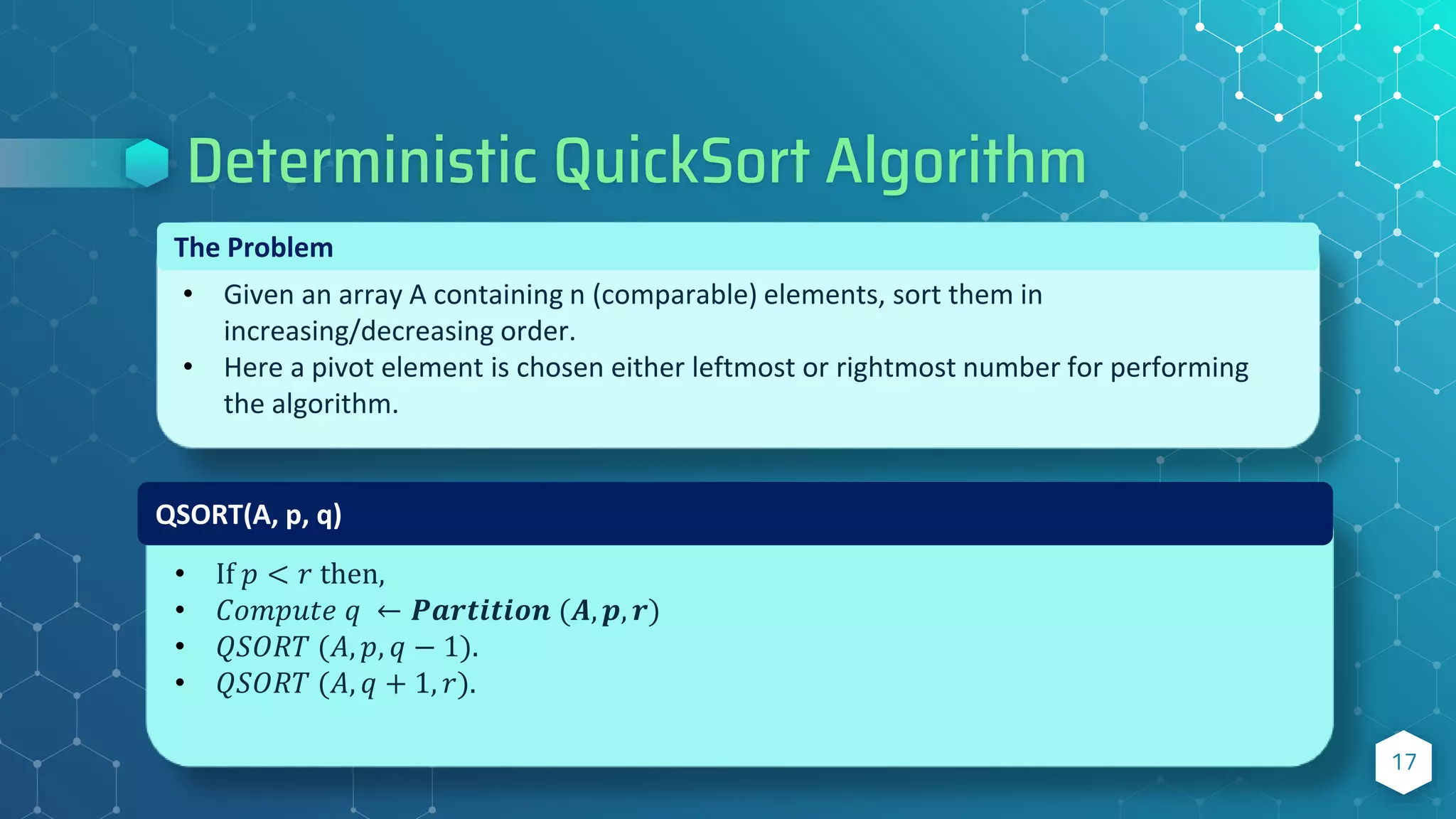
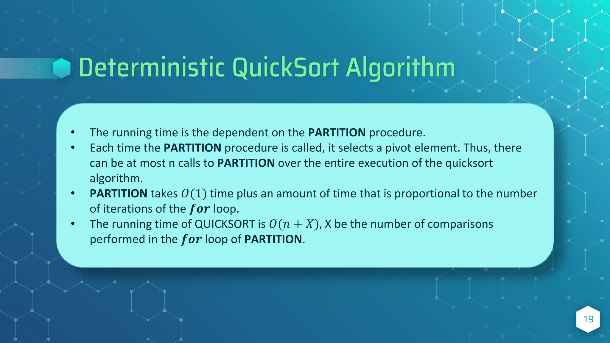
Deterministic QuickSort Algorithm 17 • Given an array A containing n (comparable) elements, sort them in increasing/decreasing order. • Here a pivot element is chosen either leftmost or rightmost number for performing the algorithm. The Problem • If 𝑝 < 𝑟 then, • 𝐶𝑜𝑚𝑝𝑢𝑡𝑒 𝑞 ← 𝑷𝒂𝒓𝒕𝒊𝒕𝒊𝒐𝒏 (𝑨, 𝒑, 𝒓) • 𝑄𝑆𝑂𝑅𝑇 (𝐴, 𝑝, 𝑞 − 1). • 𝑄𝑆𝑂𝑅𝑇 (𝐴, 𝑞 + 1, 𝑟). QSORT(A, p, q)

Deterministic QuickSort Algorithm 18 PARTITION(A, p, r) x := A[r]; i := p-1; for j = p to r-1{ if A[j] <= x then i := i+1; swap(A[i] , A[j]); } swap(A[i+1], A[r]); return i+1:

Deterministic QuickSort Algorithm 19 • The running time is the dependent on the PARTITION procedure. • Each time the PARTITION procedure is called, it selects a pivot element. Thus, there can be at most n calls to PARTITION over the entire execution of the quicksort algorithm. • PARTITION takes 𝑂(1) time plus an amount of time that is proportional to the number of iterations of the 𝒇𝒐𝒓 loop. • The running time of QUICKSORT is 𝑂(𝑛 + 𝑋), X be the number of comparisons performed in the 𝒇𝒐𝒓 loop of PARTITION.

Randomized QuickSort Algorithm 20 • In this algorithm, pick a random number and then perform An Useful Concept – random number

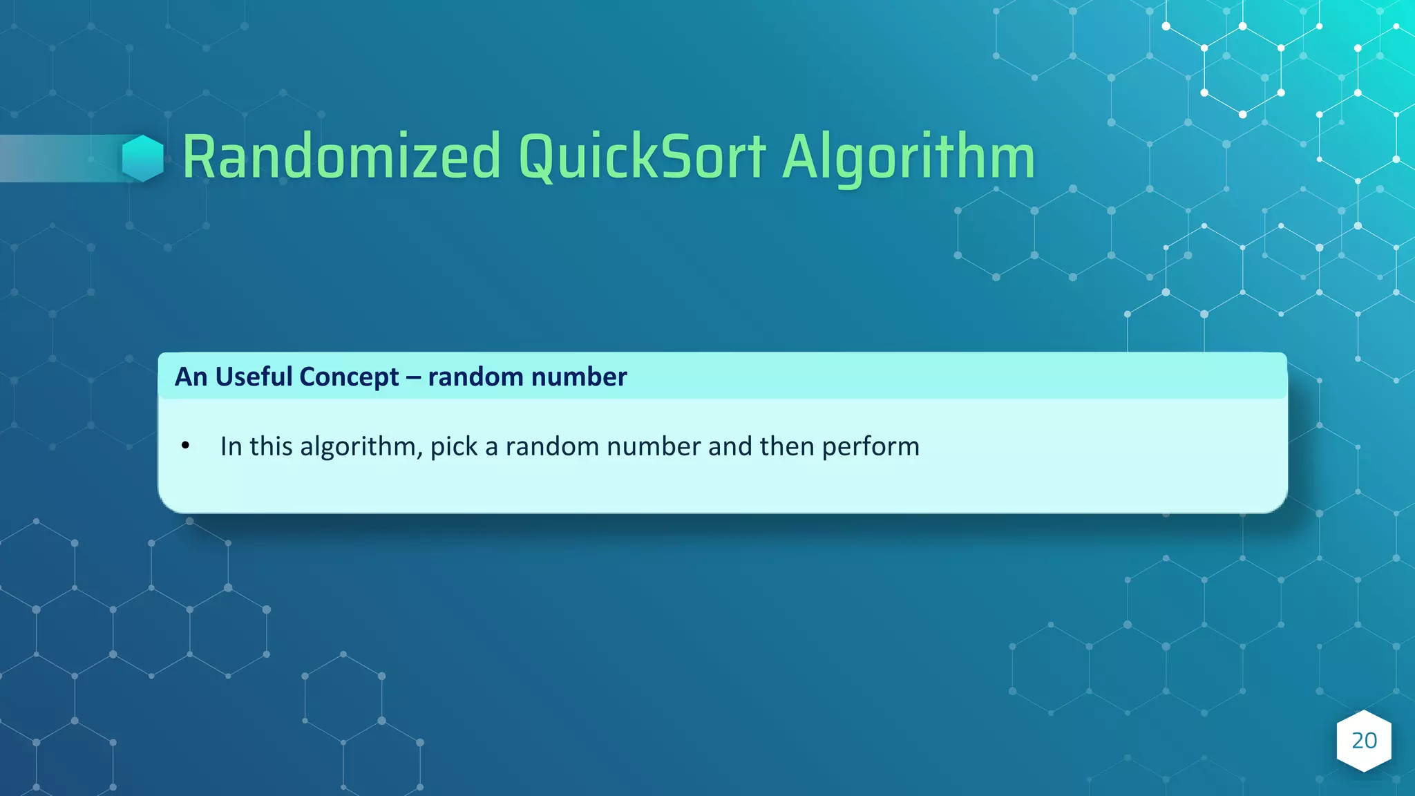
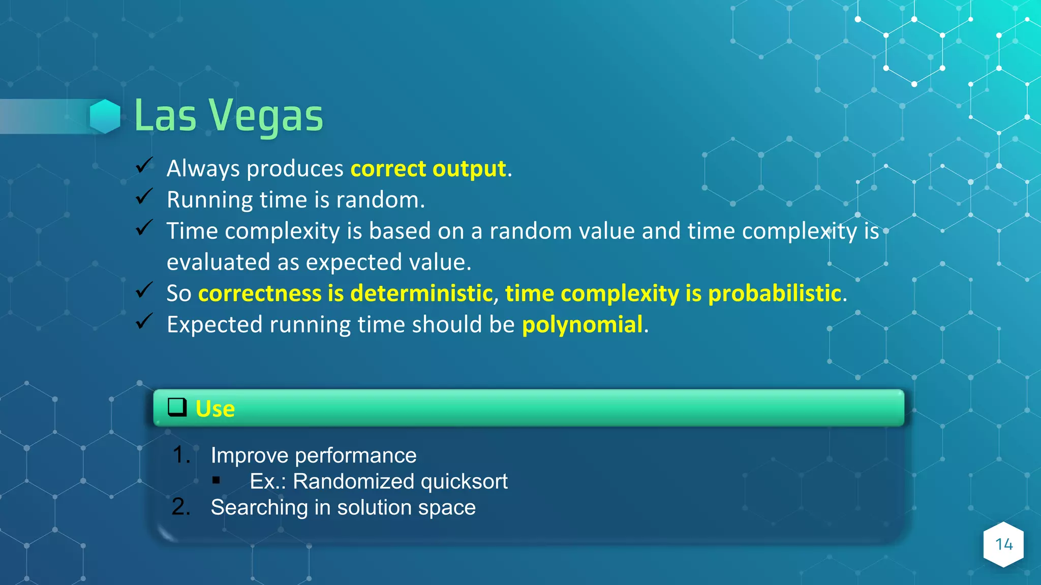
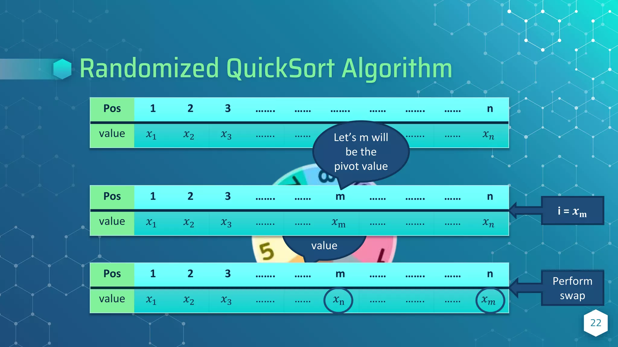
Randomized QuickSort Algorithm 21 Randomized-Quicksort(A, p, r) if p < r then q := Randomized-Partition(A, p, r); Randomized-Quicksort(A, p,q-1); Randomized-Quicksort(A,p+1,r); Randomized-Partition(A, p, r) i := Random(p, r); swap(A[i], A[r]); p := Partition(A, p, r); Return p; Almost the same as Partition as Deterministic QuickSort, but now the pivot element is not the rightmost/leftmost element, but rather an element from A[p..r] that is chosen uniformly at random.

Randomized QuickSort Algorithm 22 Pos 1 2 3 ……. …… ……. …… ……. …… n value 𝑥1 𝑥2 𝑥3 ……. …… ……. …… ……. …… 𝑥𝑛 Pick a random value Pos 1 2 3 ……. …… m …… ……. …… n value 𝑥1 𝑥2 𝑥3 ……. …… 𝑥m …… ……. …… 𝑥𝑛 Let’s m will be the pivot value Pos 1 2 3 ……. …… m …… ……. …… n value 𝑥1 𝑥2 𝑥3 ……. …… 𝑥n …… ……. …… 𝑥𝑚 i = 𝒙𝐦 Perform swap

Randomized QuickSort Algorithm 23 Goal The running time of quicksort depends mostly on the number of comparisons performed in all calls to the Randomized-Partition routine. Let X denote the random variable counting the number of comparisons in all calls to Randomized-Partition.

24 What was the main Problem in Deterministic Quicksort 1 2 … … … n Suppose given Sorted array and we have to perform here Quicksort n Pivot 1 2 … … … n n-1 1 2 … … … n n-2 1st element will be fixed position Then perform for n-1 number 2nd element will be fixed position In that case the algorithm doesn’t perform divide and conquer. This is the worse case that it has to check from 1st element to last element for every time….

25 What will be happened in case of Randomized Quicksort 1 2 3 4 5 6 4 Pick a random number 1 2 3 6 5 4 i p r Swap(A[i],A[r]) and then perform Partition function Pivot p r

26 What will be happened in case of Randomized Quicksort 1 2 3 6 5 4 i=p-1 j x 1 2 3 6 5 4 i j x 1 2 3 6 5 4 i j x 1 2 3 6 5 4 i j A[j] <= x ? No 1 2 3 6 5 4 i j A[j] <= x ? No 1 2 3 5 6 4 4 6

Comparison 27 Best Case: 𝑂 𝑛 log 𝑛 Worst Case: 𝑂 (𝑛2) Expected Case: 𝑂 𝑛 log 𝑛 Expected Worst Case: 𝑂 (𝑛2) Randomized Quicksort Deterministic Quicksort  In worst case the randomized function can pick the index of corner element every time.  But it is rare to pick the corner element.

Average runtime vs Expected runtime 28  Average runtime is averaged over all inputs of a deterministic algorithm.  Expected runtime is the expected value of the runtime random variable of a randomized algorithm.  It effectively “average” over all sequences of random numbers. Expected runtime Average runtime

Smallest Enclosing Circle 30 Problem Definition Given n points in a plane, compute the smallest radius circle that encloses all n point. Also known as minimum covering circle problem, bounding circle problem, smallest enclosing circle problem

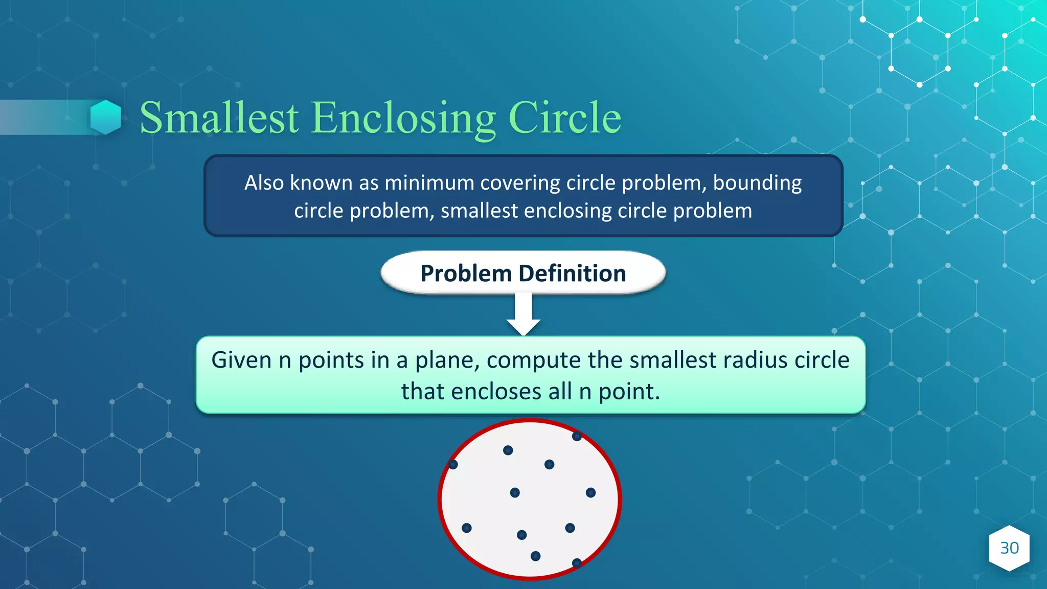
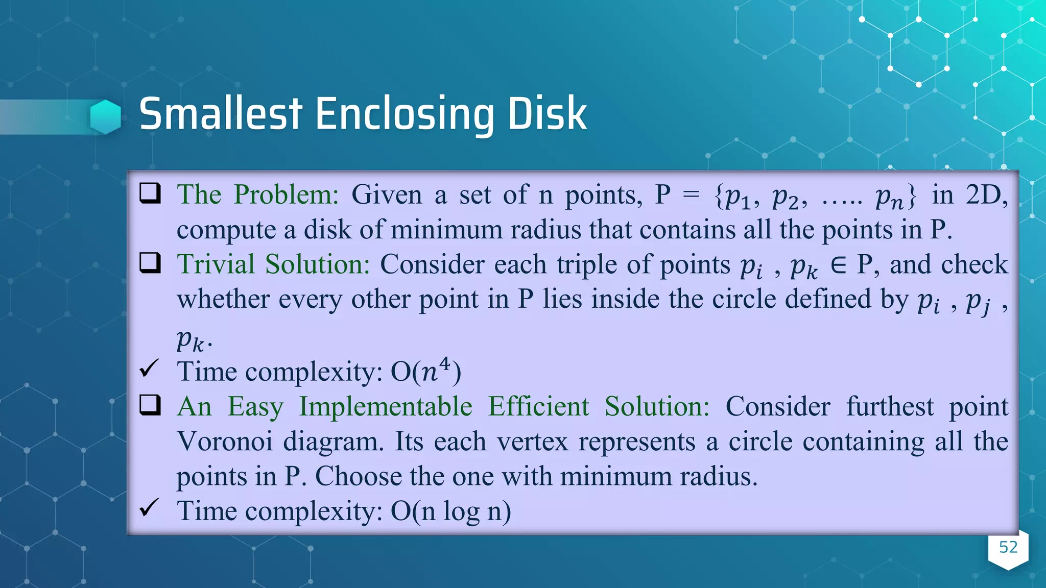
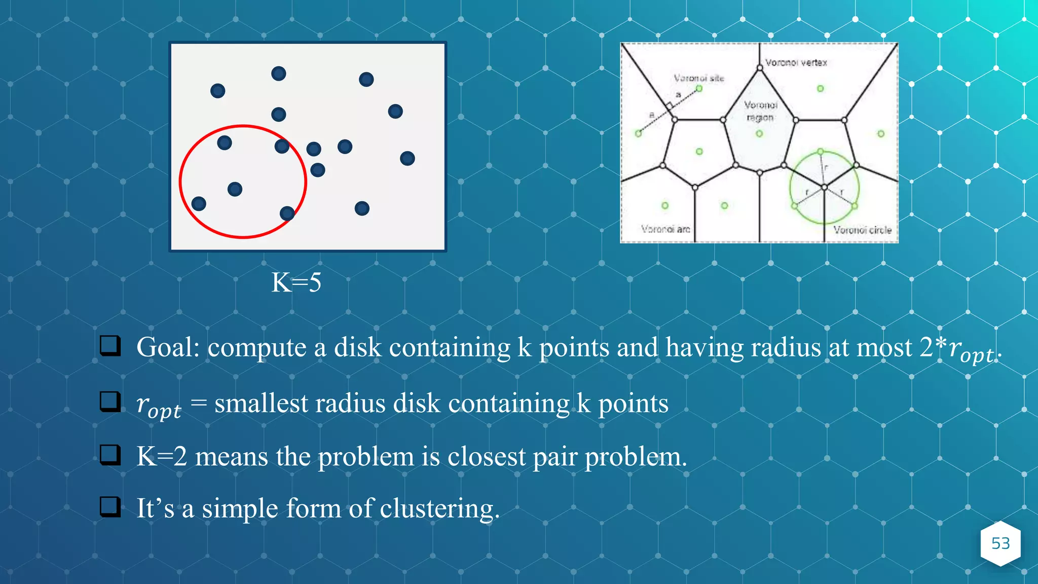
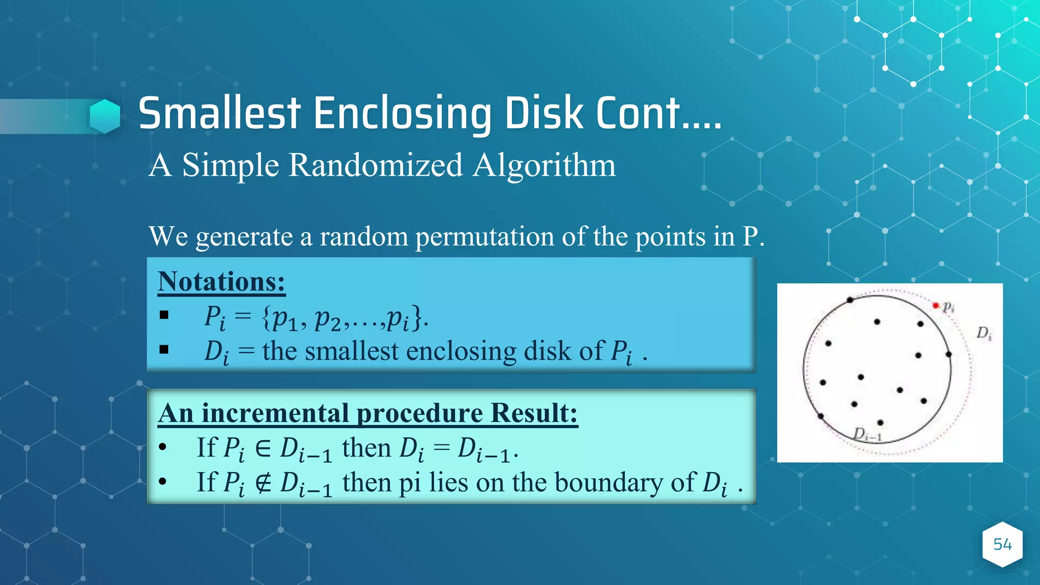
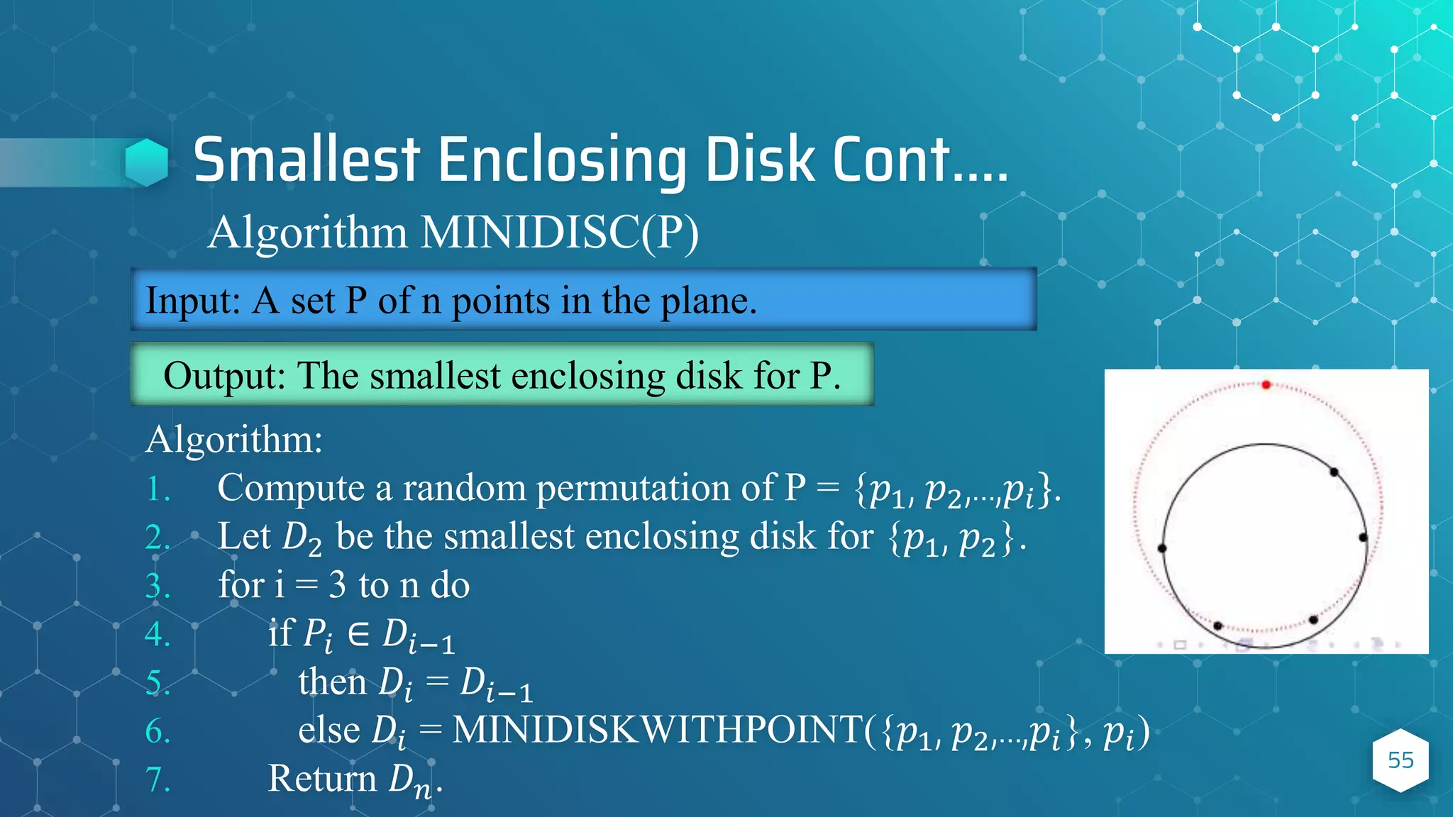
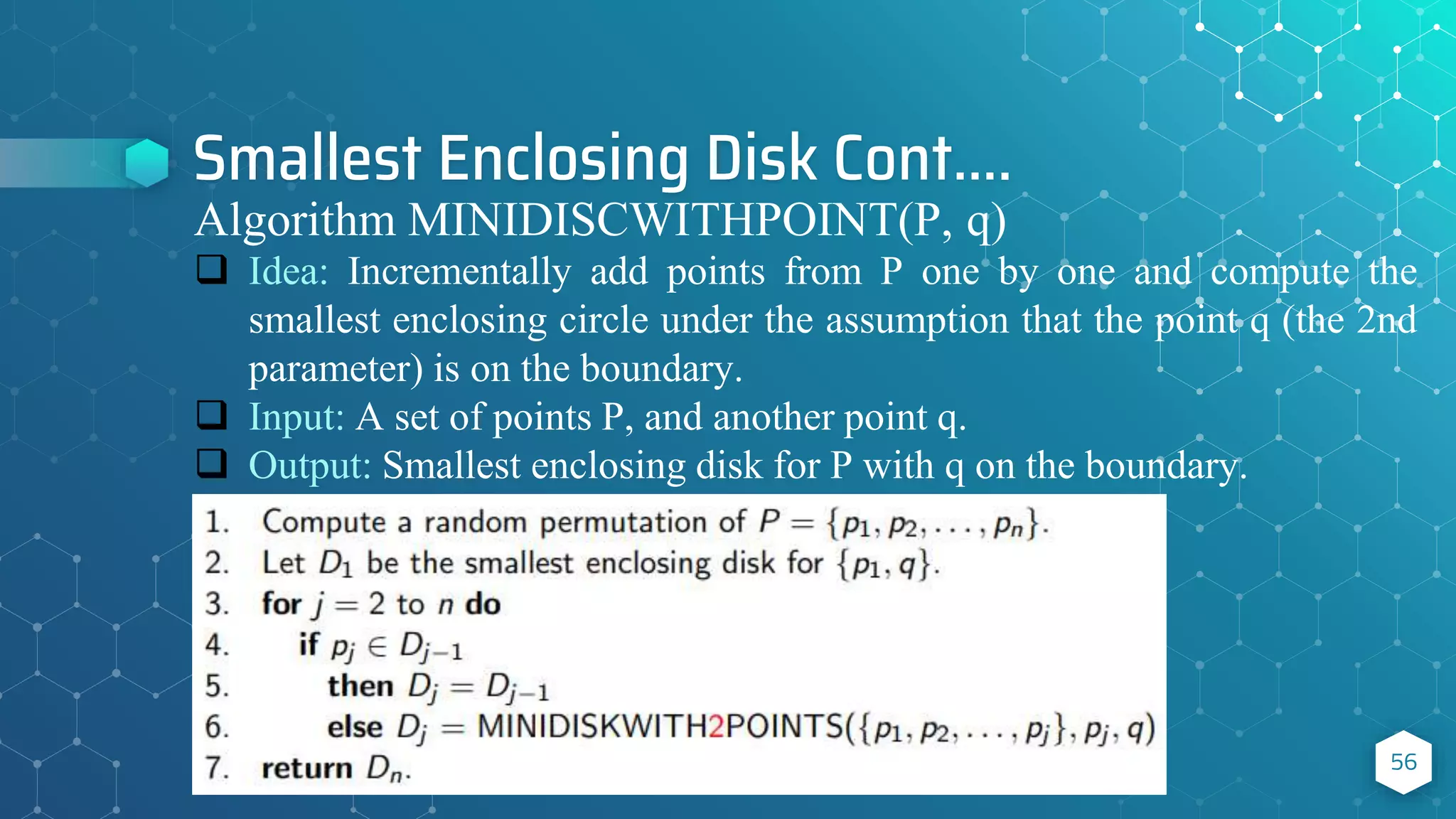
Smallest Enclosing Circle 31  Applications: Facility location problem (1-center problem)  Best deterministic algorithm : [Nimrod Megiddo, 1983] ⬦ 𝑂(𝑛3) time complexity, too complex, uses advanced geometry  Randomized Las Vegas algorithm: [Emo Welz, 1991] ⬦ Expected 𝑂(𝑛) time complexity, too simple, uses elementary geometry. ⬦ The algorithm is recursive. ⬦ Based on a linear programming algorithm of “Raimund Seidel”.

“ It may produce incorrect answer. We are able to bound its probability. By running it many times on independent random variables, we can make the failure probability arbitrarily small at the expense of running time. E.g. Randomized Mincut Algorithm 34

Monte Carlo Example ⬥ Suppose we want to find a number among n given numbers which is larger than or equal to the median. ⬥ Suppose A1 < … < An . ⬥ We want Ai , such that i ≥ n/2. It’s obvious that the best deterministic algorithm needs O(n) time to produce the answer. n may be very large! Suppose n is 100,000,000,000! ⬥ Choose 100 of the numbers with equal probability. ⬥ Find the maximum among these numbers. Return the maximum. 35

Monte Carlo Example 36  The running time of the given algorithm is O(1).  The probability of Failure is 1/(2100).  Consider that the algorithm may return a wrong answer but the probability is very smaller than the hardware failure or even an earthquake!

Michael’s Algorithms: Closest Pair of Points

38  Problem Statement: an array of n points in the plane and the problem is to find the closest pair of points in the array. Distance between two points p and q can be found by the following formula: |pq| = (𝑝𝑥 − 𝑞𝑥)2+ (𝑝𝑦 − 𝑞𝑦)2 Closest Pair of Points

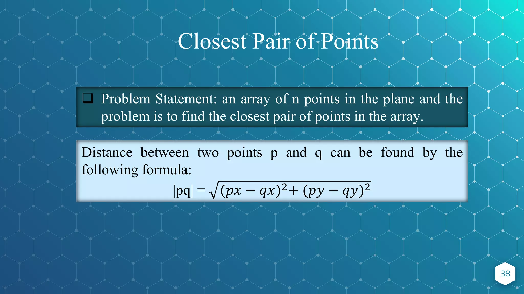
Algorithm ⬥ Input: An array of n points P[ ]. ⬥ Output: Smallest distance between two points in the given array. 39 P[ ] = {0,1, 2, 3, 4, 5, 6, 7, 8, 9, 10, 11, 12, 13, 14, 15, 16, 17}

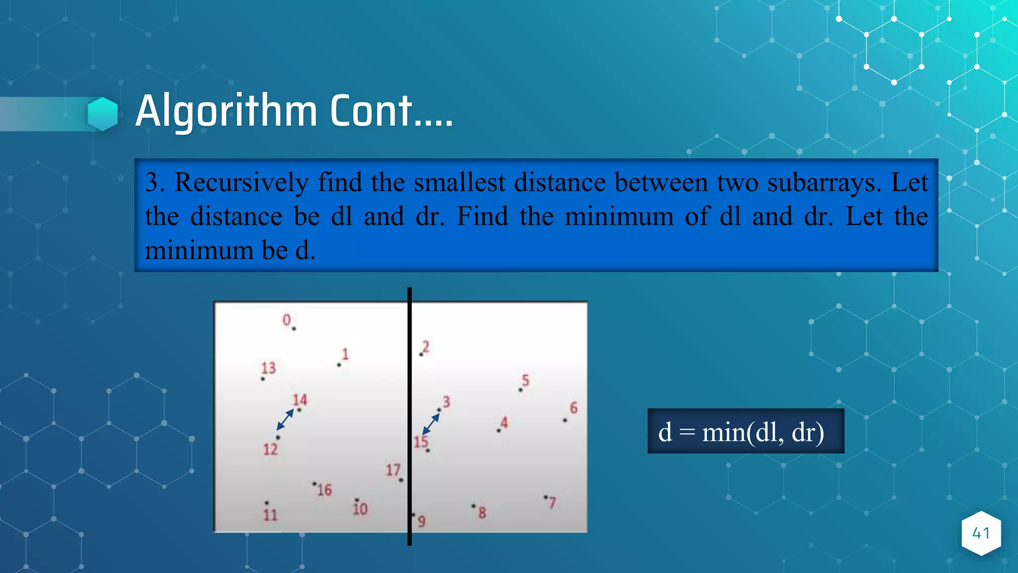
Algorithm Cont…. 40 Sort the array according to the x-coordinates at first as preprocessing step. P[ ] = {13, 12, 11, 0, 14, 16, 1, 10, 17, 9, 2, 15, 3, 8, 4, 5, 7, 6} 1. Find the middle point in sorted array. We can take P[n/2] as the middle point. P[ ] = {13, 12, 11, 0, 14, 16, 1, 10, 17, 9, 2, 15, 3, 8, 4, 5, 7, 6} 2. Divide the array in two halves. The first subarray contains points for P[0] to P[n/2] and the second subarray contains points from P[n/2+1] to P[n-1]. 𝑃𝐿 = {13, 12, 11, 0, 14, 16, 1, 10, 17} 𝑃𝑅 = {9, 2, 15, 3, 8, 4, 5, 7, 6}

Algorithm Cont…. 41 3. Recursively find the smallest distance between two subarrays. Let the distance be dl and dr. Find the minimum of dl and dr. Let the minimum be d. d = min(dl, dr)

42  Our knowledge: Insertion time depends on whether the closest pair is changed or not.  If output is the same: 1 clock tick. If output is not the same: |D| clock ticks.  With random insertion order, show that the expected total number of clock ticks used by D is O(n)

Examples of Randomized Algorithms

Minimum Cut ⬥ Min-Cut of a weighted graph is defined as the minimum sum of weights of (at least one)edges that when removed from the graph divides the graph into two groups. ⬥ The algorithm works on a method of shrinking the graph until only one node is left in the graph. ⬥ Minimum value in the list would be the minimum cut value of the graph. 44

Minimum Cut Cont.... 45 • Select the edge with minimum weight and according this minimum weight edge next move is done in e network graph. Some points are taken in consideration when working with Min-Cut: • A cut of connected graph is obstained bye dividing vertex set V of graph G into 2 sets 𝑉1 & 𝑉2. • There are no common vertices in 𝑉1 & 𝑉2, that is, two sets are disjoint. • 𝑉1 U 𝑉2 = V

Minimum Cut Cont…. Algorithm:  Repeat steps 2 to 4 until only two vertices are left.  Pick an edge e(u,v) at random.  Merge u and v.  Remove self loops from E.  Return |E|. 46 a b d c e f

48 a bd c e, f a bd c ef a, bd c ef abd c ef

49 abd c, ef abd c, ef abd c, ef

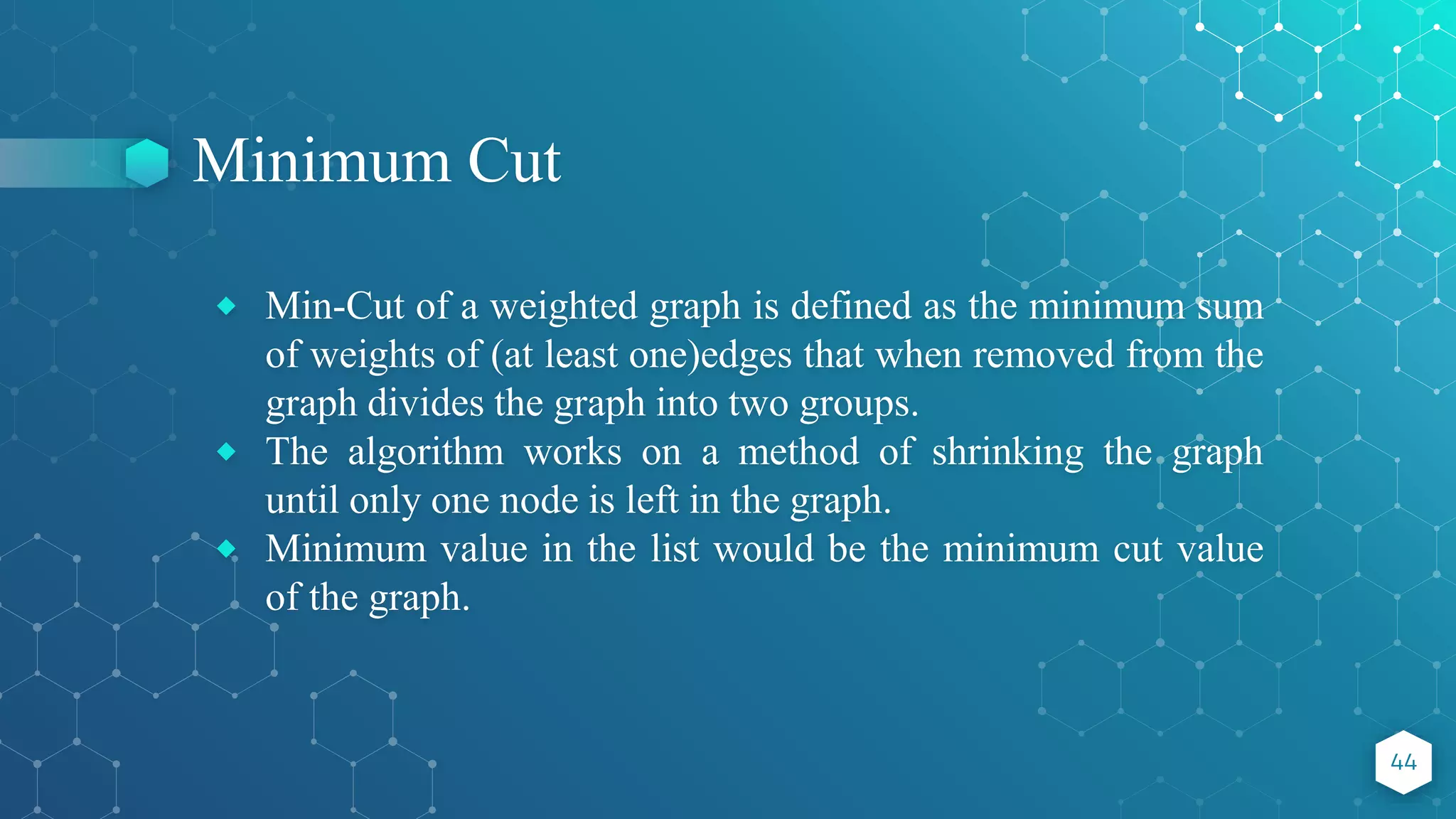
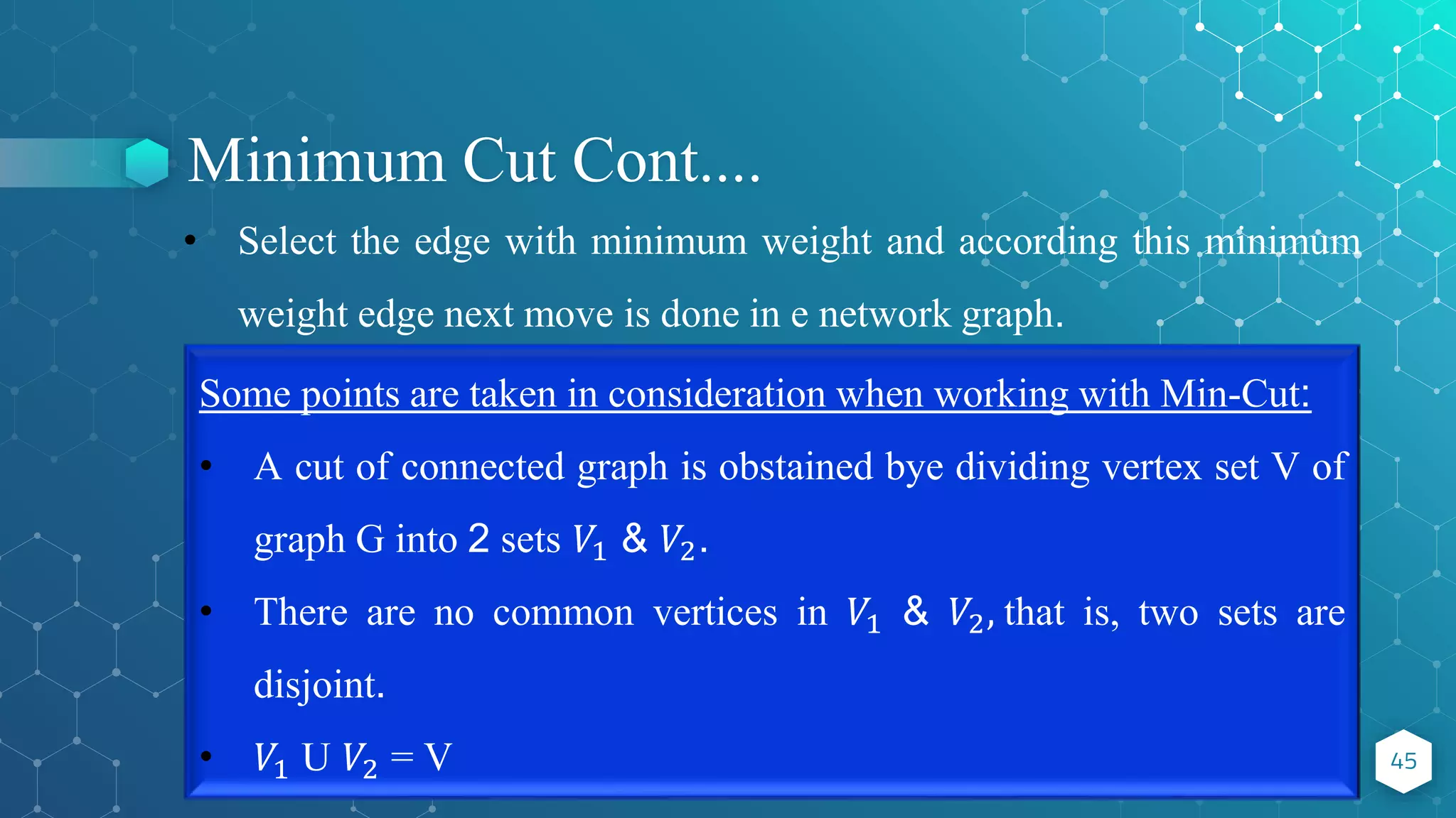
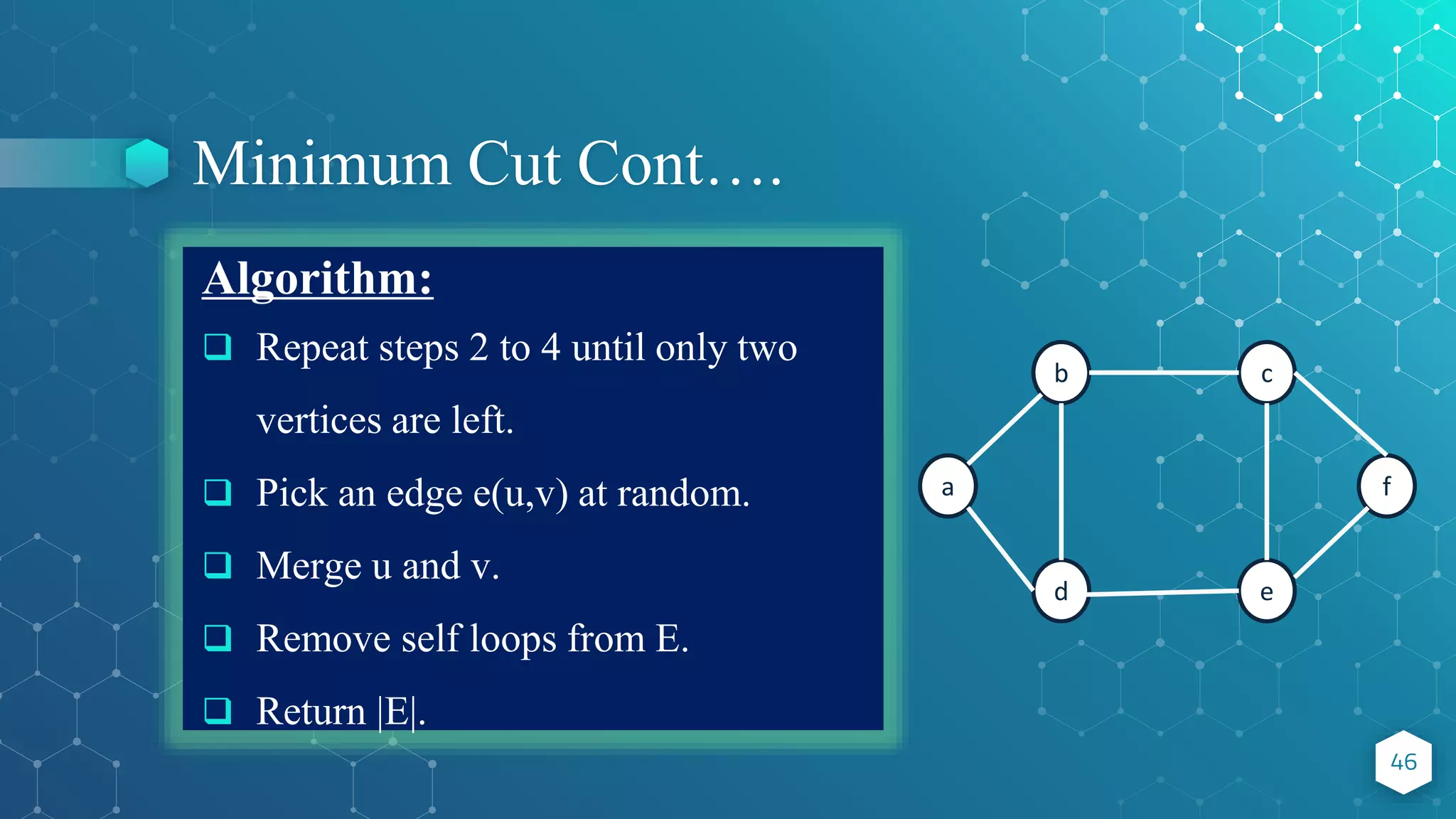
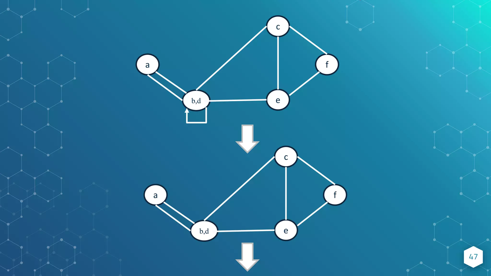
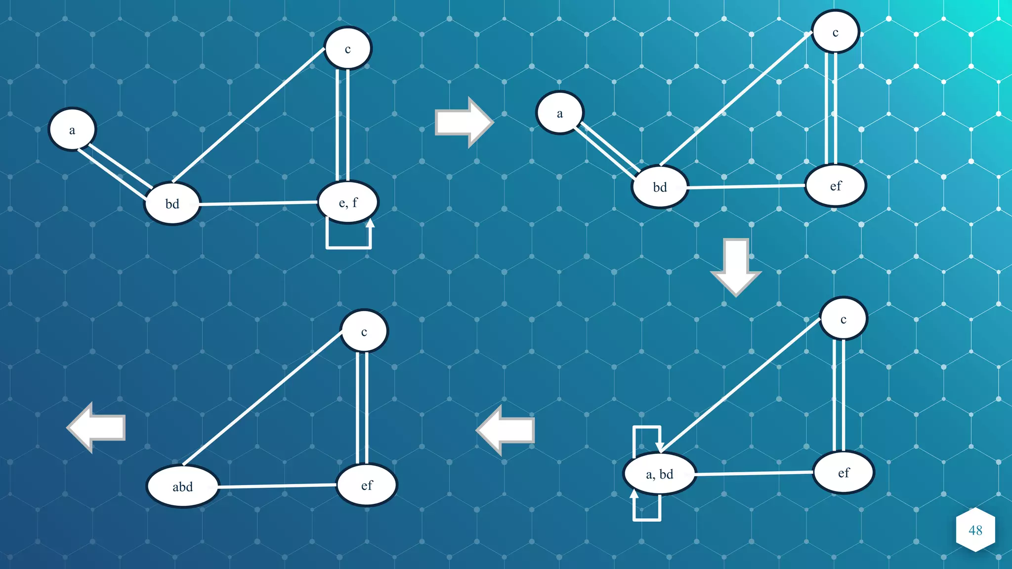
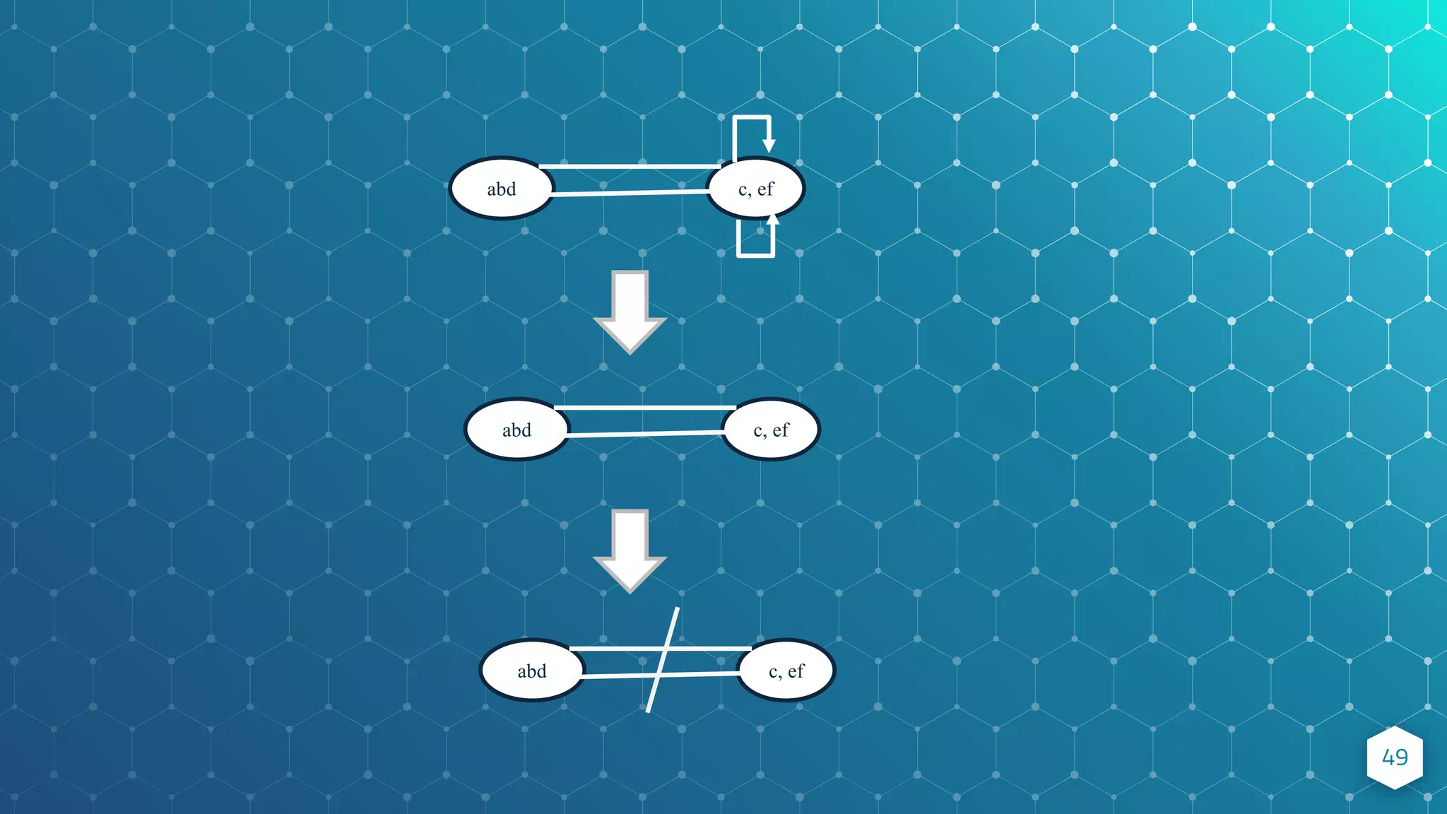
Minimum Cut 50  Problem definition: Given a connected graph G=(V,E) on n vertices and m edges, compute the smallest set of edges that will make G disconnected.  Best deterministic algorithm : [Stoer and Wagner, 1997] • O(mn) time complexity.  Randomized Monte Carlo algorithm: [Karger, 1993] • O(m log n) time complexity.  Error probability: n−𝑐 for any 𝑐 that we desire.

Applications of Minimum Cut Algorithm 51  Partitioning items in a database,  Identify clusters of related documents,  Network reliability,  Network design,  Circuit design, etc.

Smallest Enclosing Disk 52  The Problem: Given a set of n points, P = {𝑝1, 𝑝2, ….. 𝑝𝑛} in 2D, compute a disk of minimum radius that contains all the points in P.  Trivial Solution: Consider each triple of points 𝑝𝑖 , 𝑝𝑘 ∈ P, and check whether every other point in P lies inside the circle defined by 𝑝𝑖 , 𝑝𝑗 , 𝑝𝑘.  Time complexity: O(𝑛4)  An Easy Implementable Efficient Solution: Consider furthest point Voronoi diagram. Its each vertex represents a circle containing all the points in P. Choose the one with minimum radius.  Time complexity: O(n log n)

53  Goal: compute a disk containing k points and having radius at most 2*𝑟𝑜𝑝𝑡.  𝑟𝑜𝑝𝑡 = smallest radius disk containing k points  K=2 means the problem is closest pair problem.  It’s a simple form of clustering. K=5

Smallest Enclosing Disk Cont…. 54 A Simple Randomized Algorithm We generate a random permutation of the points in P. Notations:  𝑃𝑖 = {𝑝1, 𝑝2,…,𝑝𝑖}.  𝐷𝑖 = the smallest enclosing disk of 𝑃𝑖 . An incremental procedure Result: • If 𝑃𝑖 ∈ 𝐷𝑖−1 then 𝐷𝑖 = 𝐷𝑖−1. • If 𝑃𝑖 ∉ 𝐷𝑖−1 then pi lies on the boundary of 𝐷𝑖 .

Smallest Enclosing Disk Cont…. Algorithm: 1. Compute a random permutation of P = {𝑝1, 𝑝2,…,𝑝𝑖}. 2. Let 𝐷2 be the smallest enclosing disk for {𝑝1, 𝑝2}. 3. for i = 3 to n do 4. if 𝑃𝑖 ∈ 𝐷𝑖−1 5. then 𝐷𝑖 = 𝐷𝑖−1 6. else 𝐷𝑖 = MINIDISKWITHPOINT({𝑝1, 𝑝2,…,𝑝𝑖}, 𝑝𝑖) 7. Return 𝐷𝑛. 55 Algorithm MINIDISC(P) Input: A set P of n points in the plane. Output: The smallest enclosing disk for P.

Smallest Enclosing Disk Cont…. 56 Algorithm MINIDISCWITHPOINT(P, q)  Idea: Incrementally add points from P one by one and compute the smallest enclosing circle under the assumption that the point q (the 2nd parameter) is on the boundary.  Input: A set of points P, and another point q.  Output: Smallest enclosing disk for P with q on the boundary.

Smallest Enclosing Disk Cont…. 57 Algorithm MINIDISCWITH2POINT(P, 𝑞1, 𝑞2)  Idea: Thus we have two fixed points; so we need to choose another point among P {q1, q2} to have the smallest enclosing disk containing P.

Time Complexity 58  MINIDISKWITHPOINTS needs O(n) time if we do not consider the time taken in the call of the routine MINIDISKWITH2POINTS. Worst case: O(𝑛3 ) Expected case: MINIDISKWITH2POINTS needs O(n) time.

Primality Testing 59 Algorithm: for i = 2 to N-1 { if (x mod i == 0) return -1 } return 1 Time Complexity: O(N) Mathematical Result: 2, ….. , 𝑁 Prime Number: divisible only by 1 and the number itself. Ex: 1, 2, 3, 5, 7, 11, ………

Primality Testing Cont…. 60 Algorithm: for i = 2 to 𝑁 { if (x mod i == 0) return -1 } return 1 Time Complexity: O( 𝑁)

Primality Testing Cont…. 61 Fermat’s Theorem: If n is prime, then 𝑎𝑛−1 ≡ 1 (mod n) for any integer a < n. n = 3 , a = 2, then 22 % 3 = 4 % 3 = 1 n = 5, a = 2, then 25−1 % 5 = 16 % 5 = 1 n = 5, a = 3, then 35−1 % 5 = 81 % 5 = 1

Primality Testing Cont…. 62 Algorithm: if((𝑎𝑛−1)% = = 1) for(i = 1 to large) do { a = random (n) 1, ………, n-1 z = 𝑎𝑛−1 if((z%n) ≠ 1) return False } return True Input: Prime = n Sufficient number of integers a < n

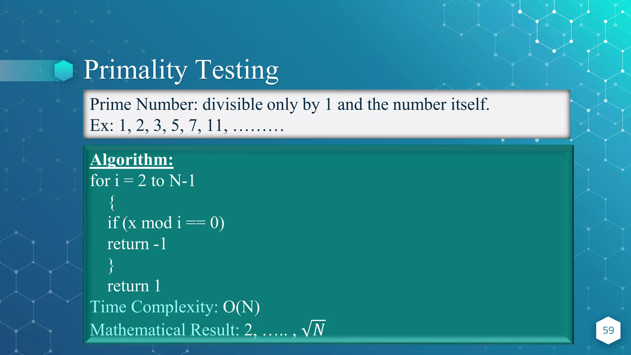
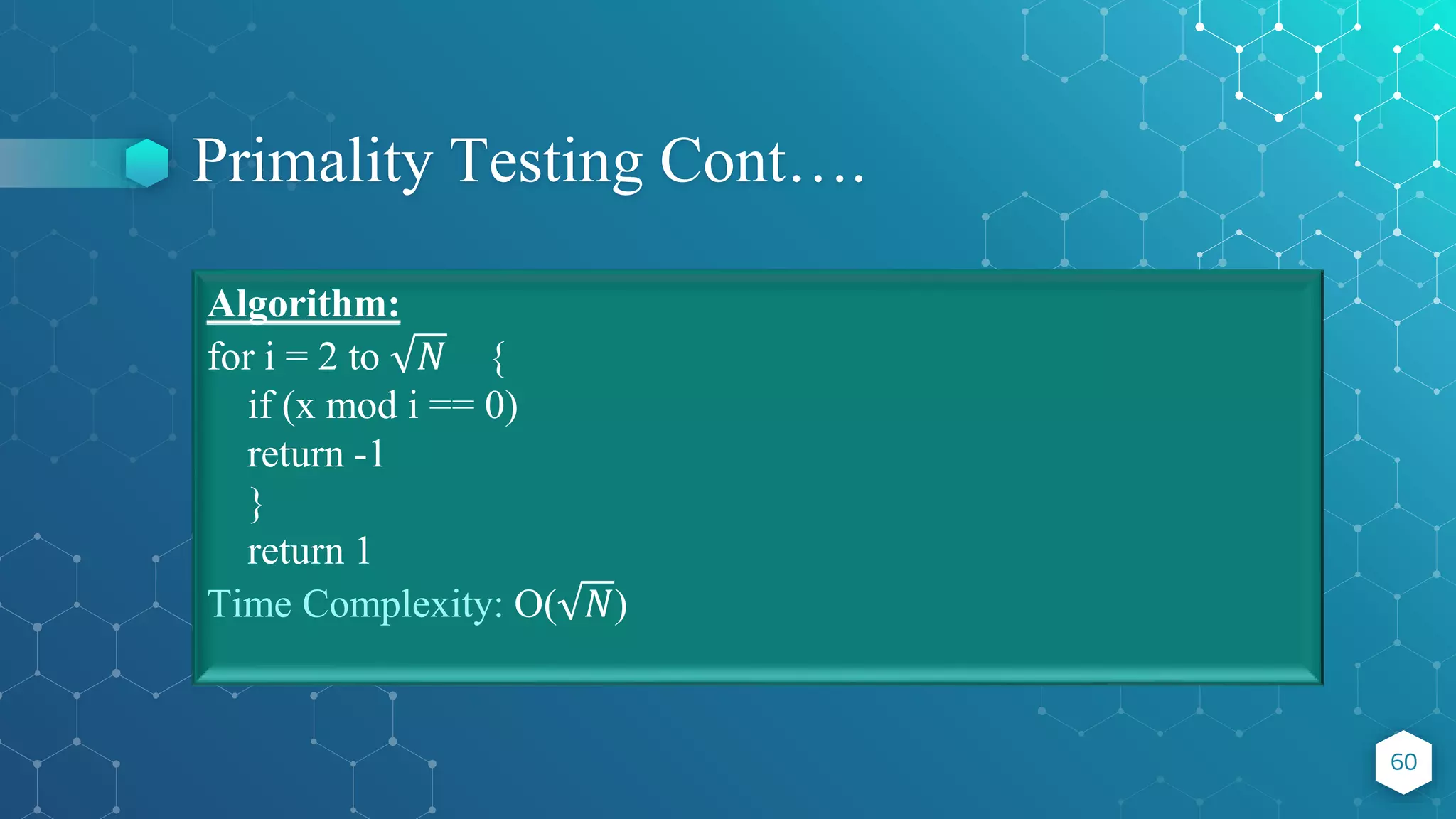
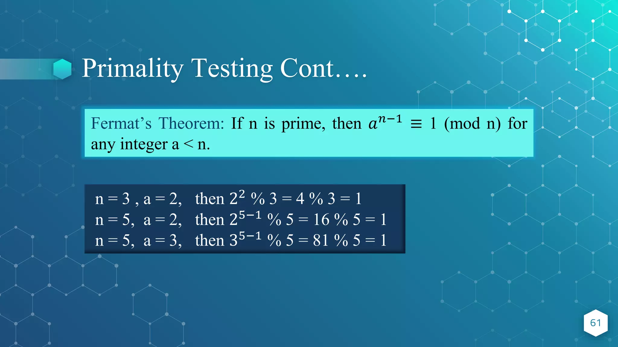
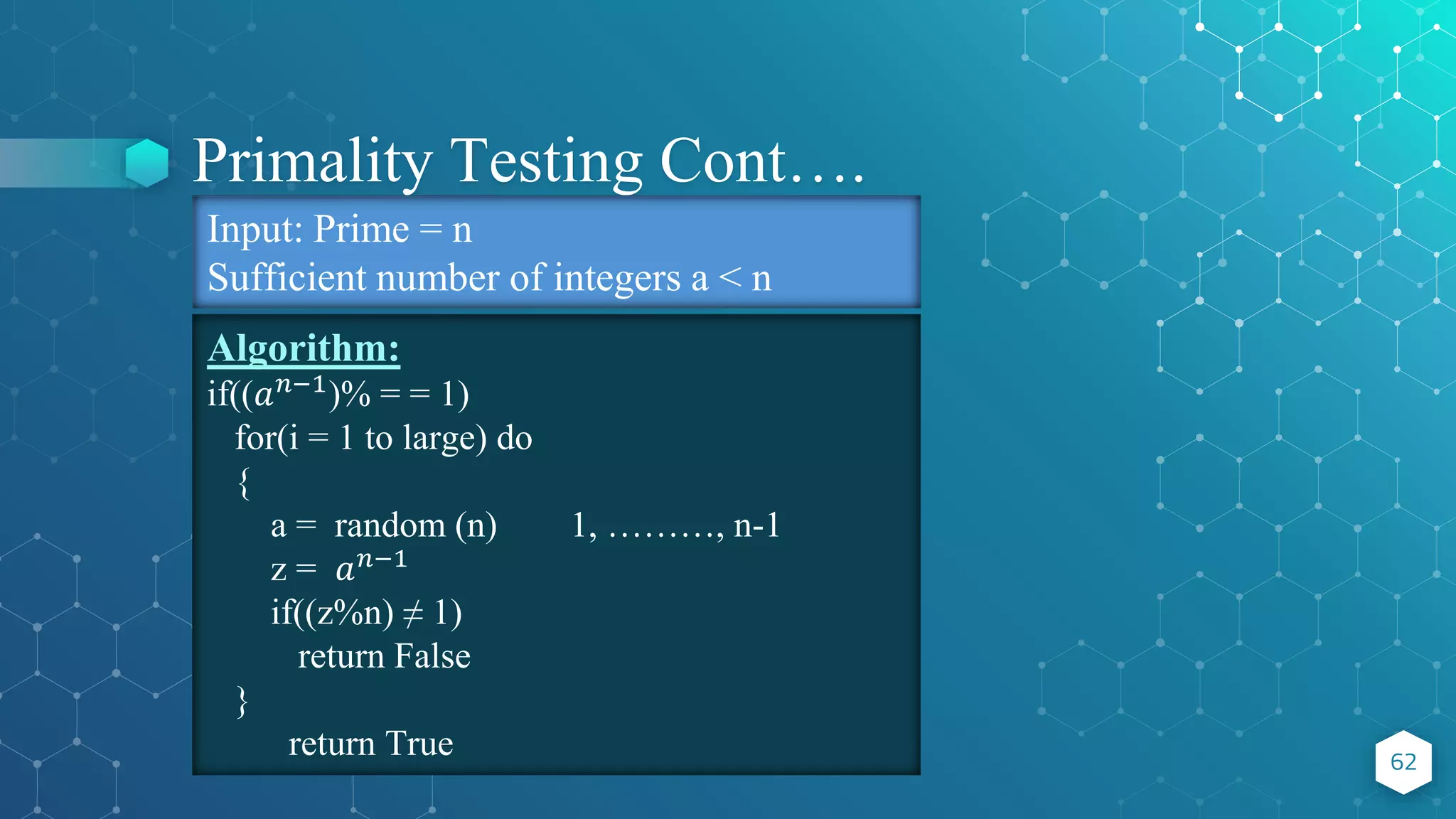
Primality Testing 63  Applications:  RSA-cryptosystem  Algebraic algorithms  Best deterministic algorithm : [Agrawal, Kayal and Saxena,  O(n6 ) time complexity.  Randomized Monte Carlo algorithm: [Rabin, 1980]  O(k n2 ) time complexity.  Error probability: 2−k for any k that we desire. For 𝐧= 50, this probability is 𝟏𝟎−𝟏𝟓

Randomized Data Structure -Boom Filter

“ ⬥ A randomized data structure for fast searching ⬥ Keys represented in compressed storage as bit array ⬥ Two operations supported – Insert and Search ⬥ Search returns YES (present) or NO (not present) ⬥ NO is always correct YES is correct with a probability ⬥ Similar to Monte Carlo with one-sided error ⬥ Many practical applications in networks, content search etc. 65

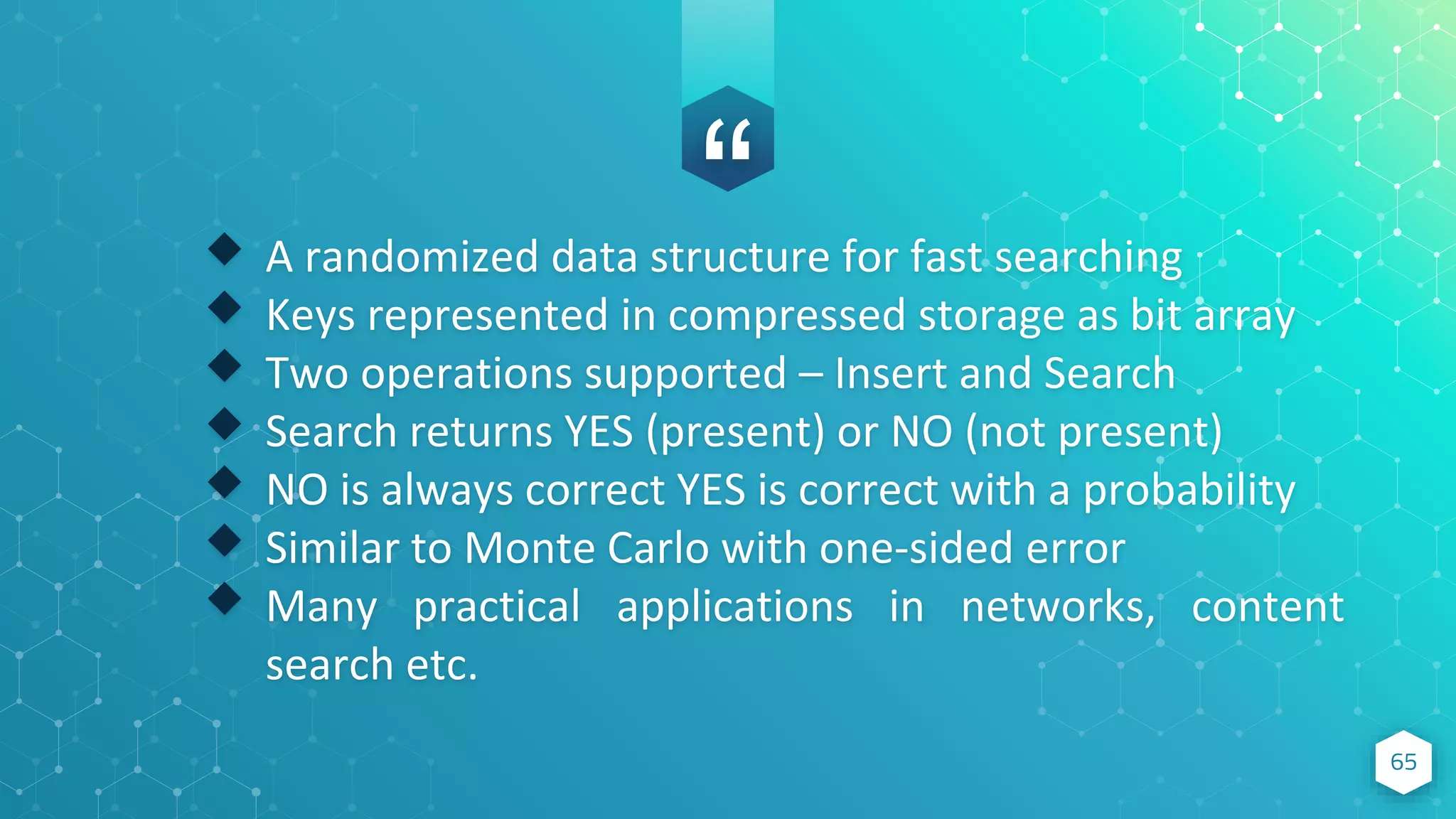
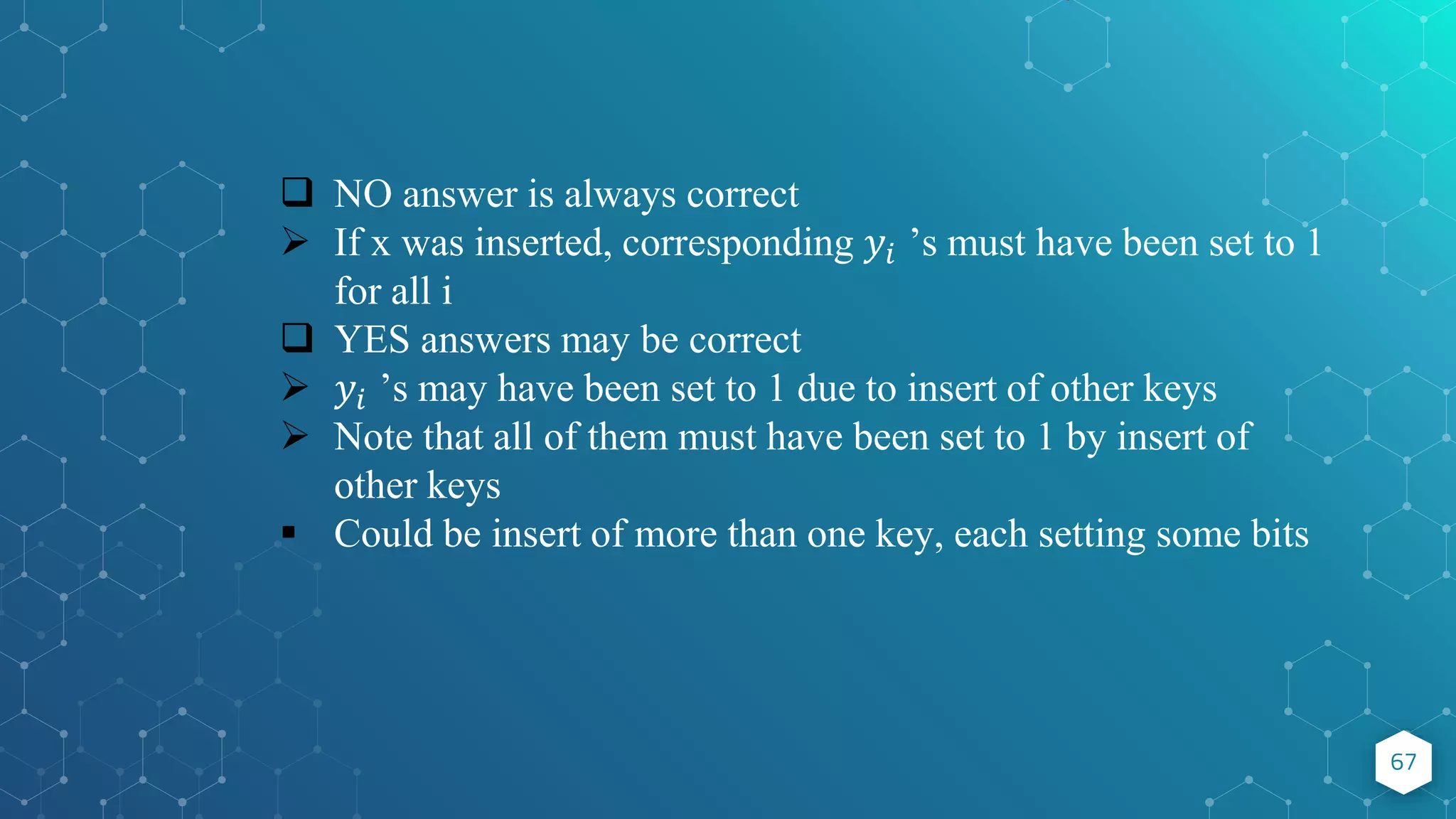
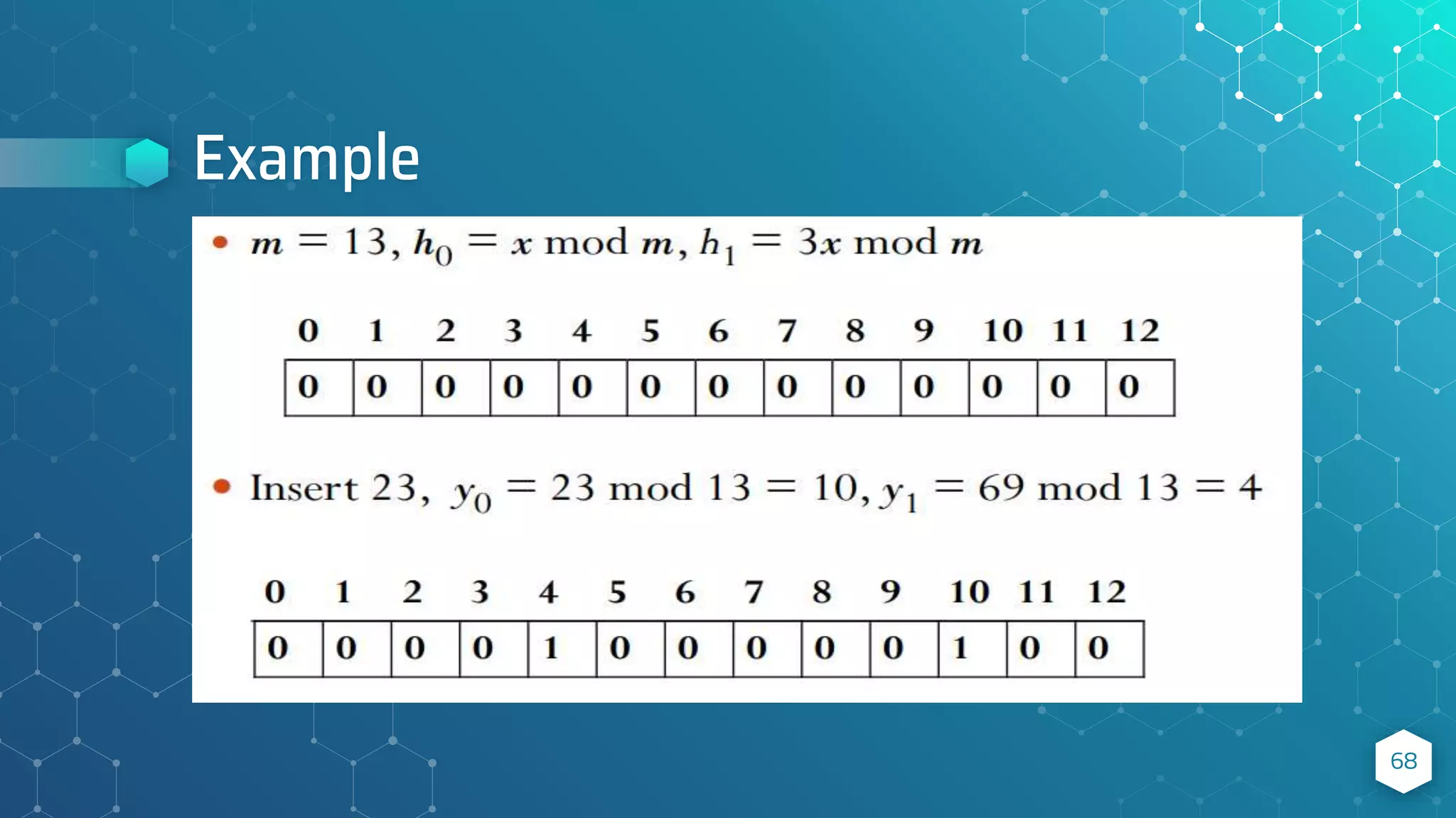
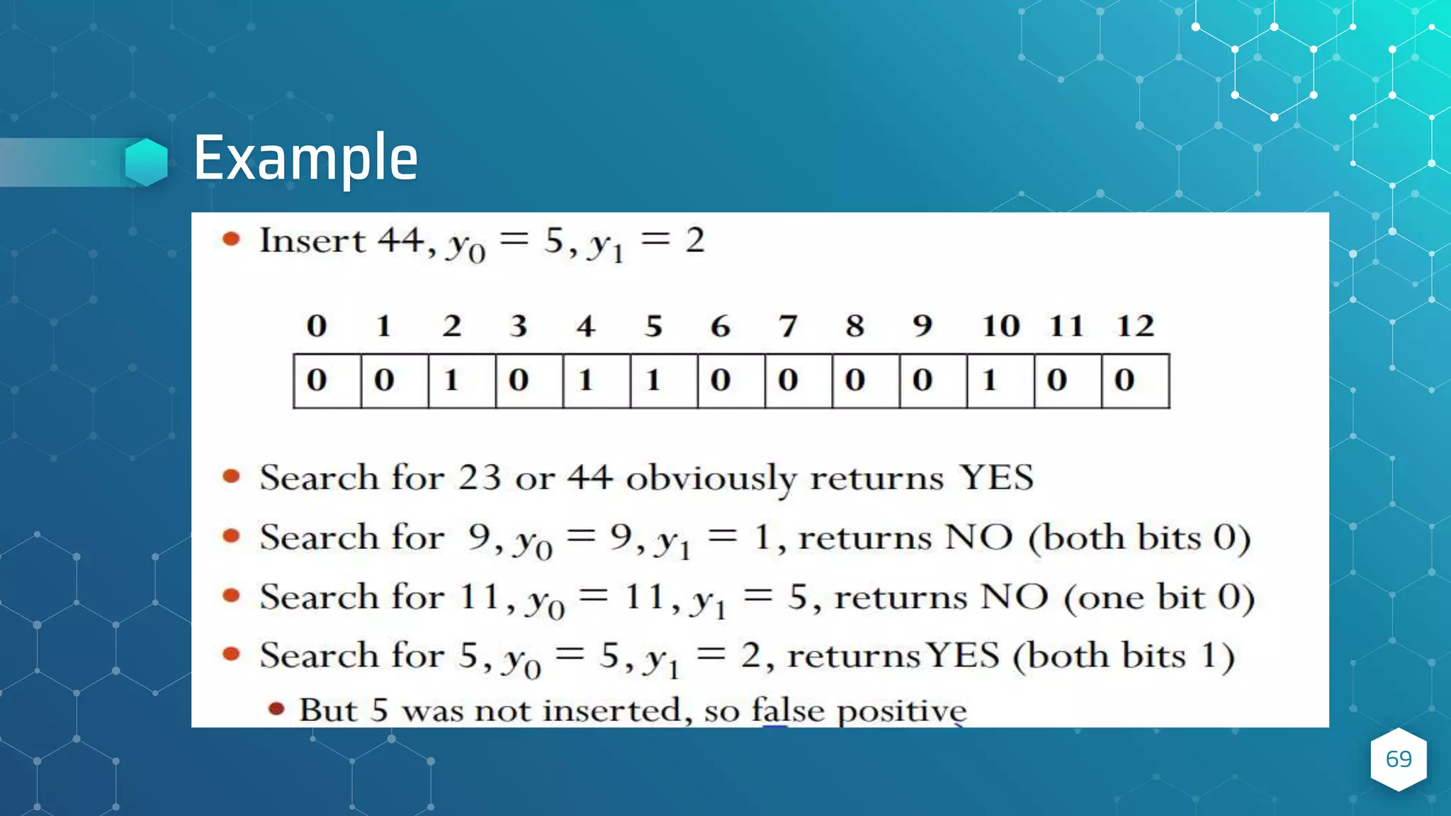
Bloom Filter Operation 66  A bit array A[0..m-1] of size m  Initially all bits are set to 0  A set of k random and independent hash functions ℎ0, ℎ1, …,ℎ𝑘−1 producing a hash value between 0 and m – 1  Insert key x  Compute 𝑦𝑖 = ℎ𝑖(x) for i = 0, 1,….,k – 1  Set A[𝑦𝑖] = 1 for i = 0, 1, …,k – 1  (𝑦0, 𝑦1, 𝑦2,…,𝑦𝑘−1) is called the signature of x  Search for a key x  Compute 𝑦𝑖 = hi (x) for i = 0, 1,…,k – 1  Answer YES if A[𝑦𝑖 ] =1 for all i, NO otherwise

67  NO answer is always correct  If x was inserted, corresponding 𝑦𝑖 ’s must have been set to 1 for all i  YES answers may be correct  𝑦𝑖 ’s may have been set to 1 due to insert of other keys  Note that all of them must have been set to 1 by insert of other keys  Could be insert of more than one key, each setting some bits

70 Classifying Randomized Algorithms by Their Methods  Avoiding Worst-Case Inputs: Obtained by hiding the details of the algorithm from the adversary. Since the algorithm is chosen randomly, he can’t pick an input that is bad for all of them.  Sampling: Randomness is used for choosing a simple random sample, without replacement, of k items from a population of unknown size n in a single pass over the items. In this way, the adversary can’t direct us to non-representative samples.

71 Classifying Randomized Algorithms by Their Methods  Hashing: Obtained by selecting a hash function at random from a family of hash functions. This guarantees a low number of collisions in expectation, even if the data is chosen by an adversary.  Building Random Structures: By creating a randomized algorithm to create structures, the probability can be reached to substantial.  Symmetry Breaking: Randomization can break the deadlocks of making the progress of multiple processes stymied.

Advantages of Randomized Algorithms 72  The algorithm is usually simple and easy to implement,  The algorithm is fast with very high probability, and  It produces optimum output with very high probability.

Difficulties in Randomized Algorithm 73  There is a finite probability of getting incorrect answer. However, the probability of getting a wrong answer can be made arbitrarily small by the repeated employment of randomness.  Analysis of running time or probability of getting a correct answer is usually difficult.  Getting truly random numbers is impossible. One needs to depend on pseudo random numbers. So, the result highly depends on the quality of the random numbers.  Its quality depends on quality of random number generator used as part of the algorithm.  The other disadvantage of randomized algorithm is hardware failure.

75 Tool for sorting: Randomized Quick Sort, then there is no user that always gets worst case. Everybody gets expected O(n Log n) time. Cryptography: Randomized algorithms have huge applications in Cryptography, e.g: RSA Crypto-System. Load Balancing. Number-Theoretic Applications: Primality Testing Data Structures: Hashing, Sorting, Searching, Order Statistic and Computational Geometry. Algebraic identities: Polynomial and matrix identity verification. Interactive proof systems. Application

76 Mathematical programming: Faster algorithms for linear programming, Rounding linear program solutions to integer program solutions Graph algorithms: Minimum spanning trees, shortest paths, minimum cuts. Counting and enumeration: Matrix permanent Counting combinatorial structures. Parallel and distributed computing: Deadlock avoidance distributed consensus. Probabilistic existence proofs: Show that a combinatorial object arises with non-zero probability among objects drawn from a suitable probability space. Application

Randomized Algorithm- Advanced Algorithm

More Related Content

What's hot

Similar to Randomized Algorithm- Advanced Algorithm

More from Mahbubur Rahman

Recently uploaded

Randomized Algorithm- Advanced Algorithm