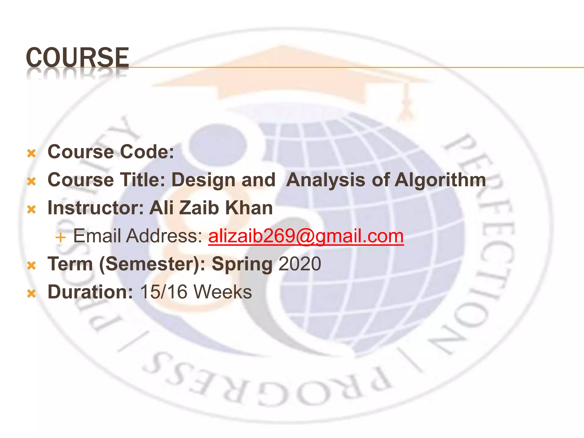
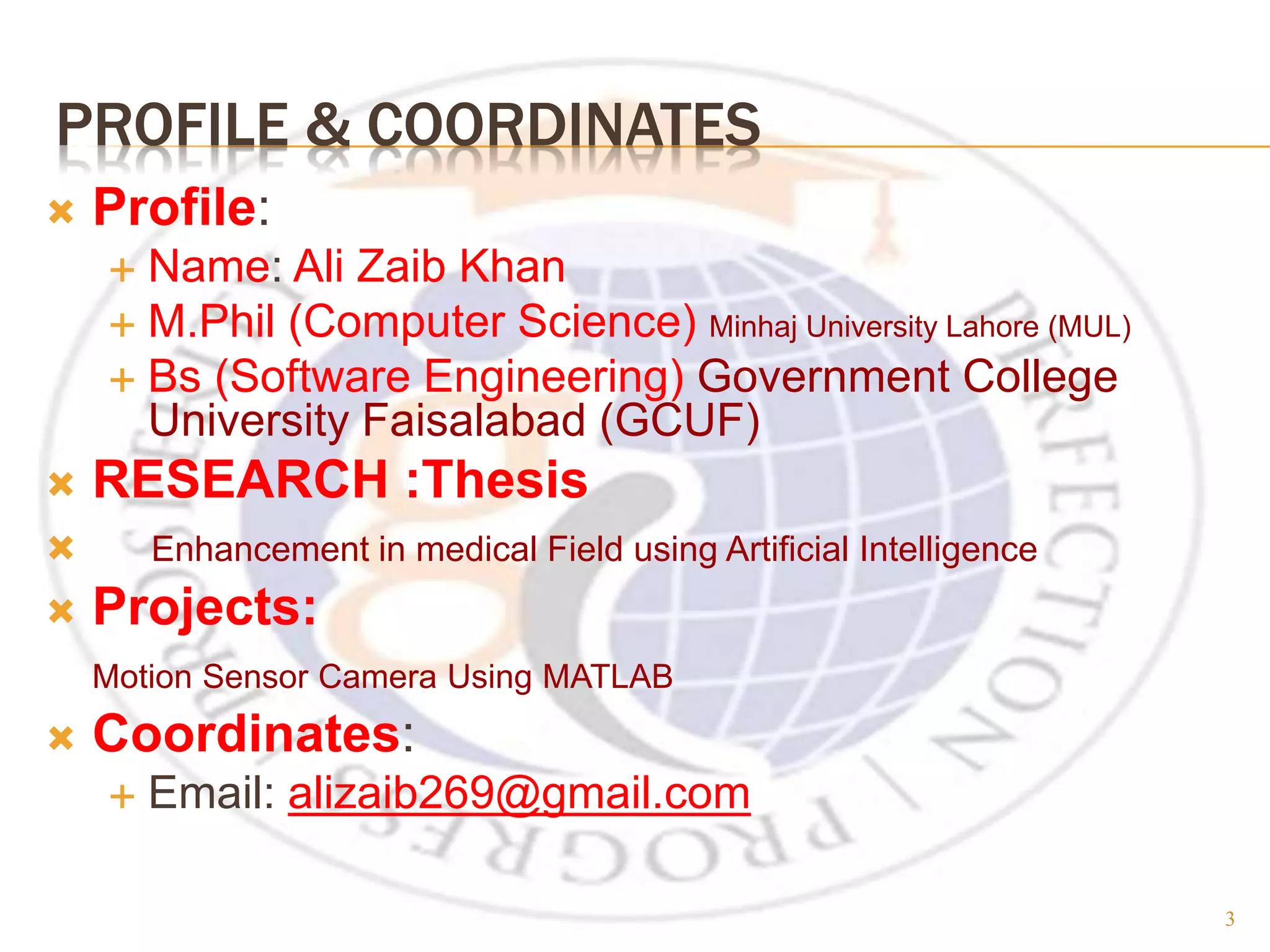
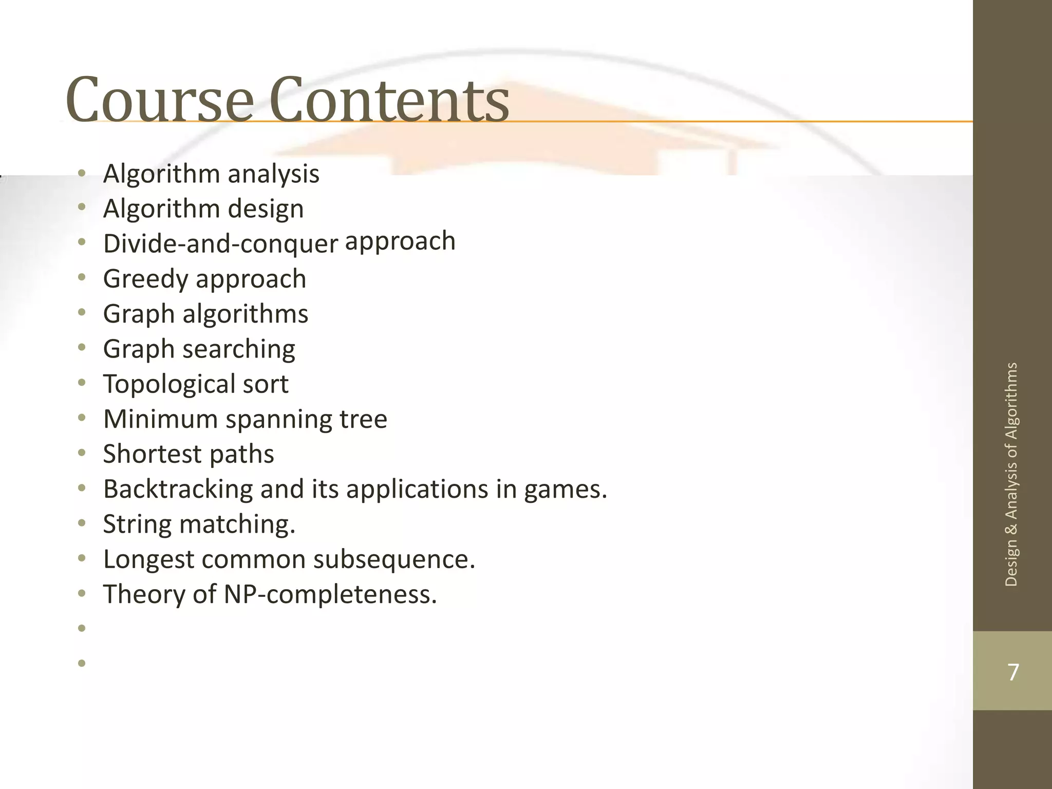
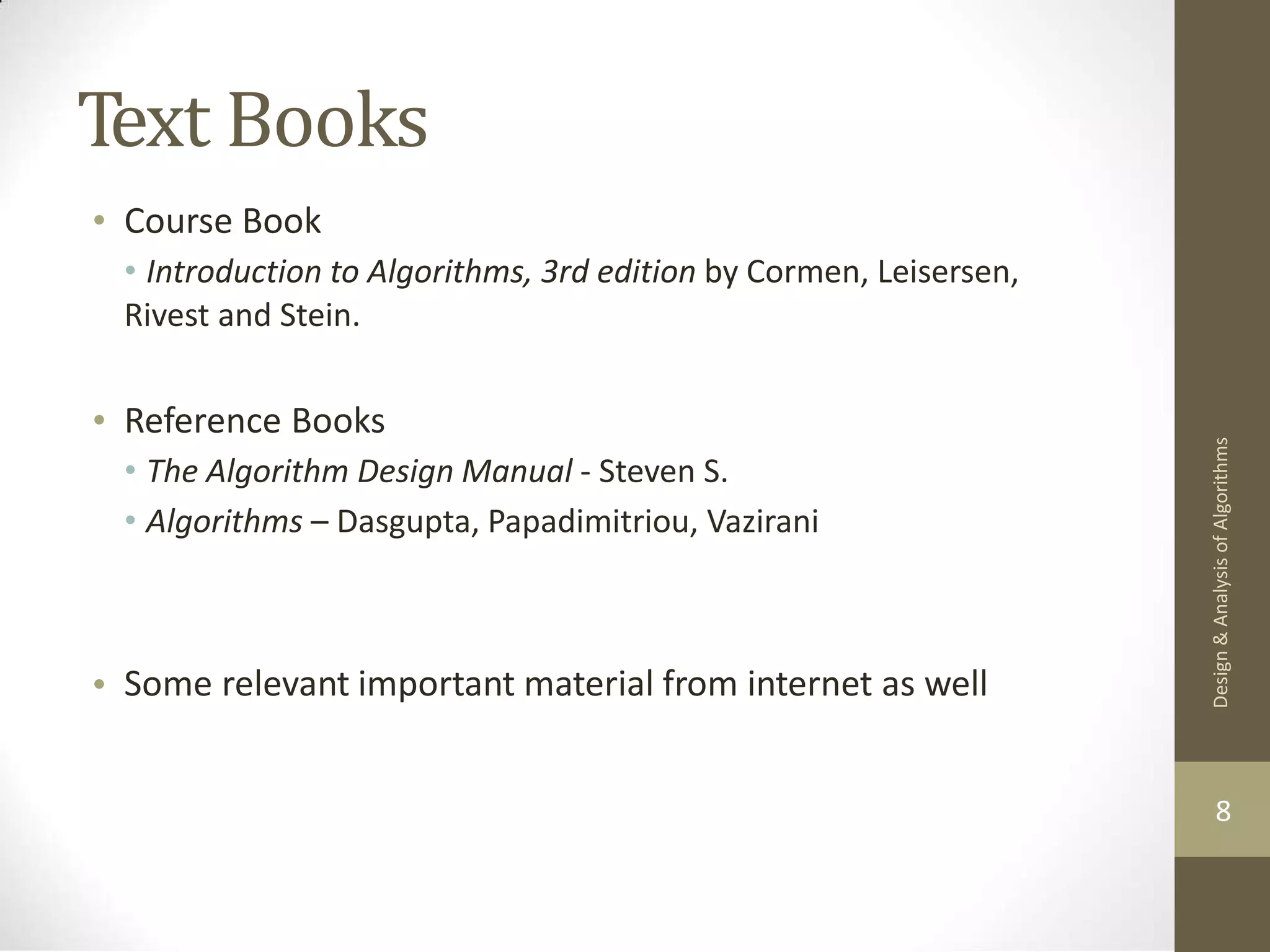
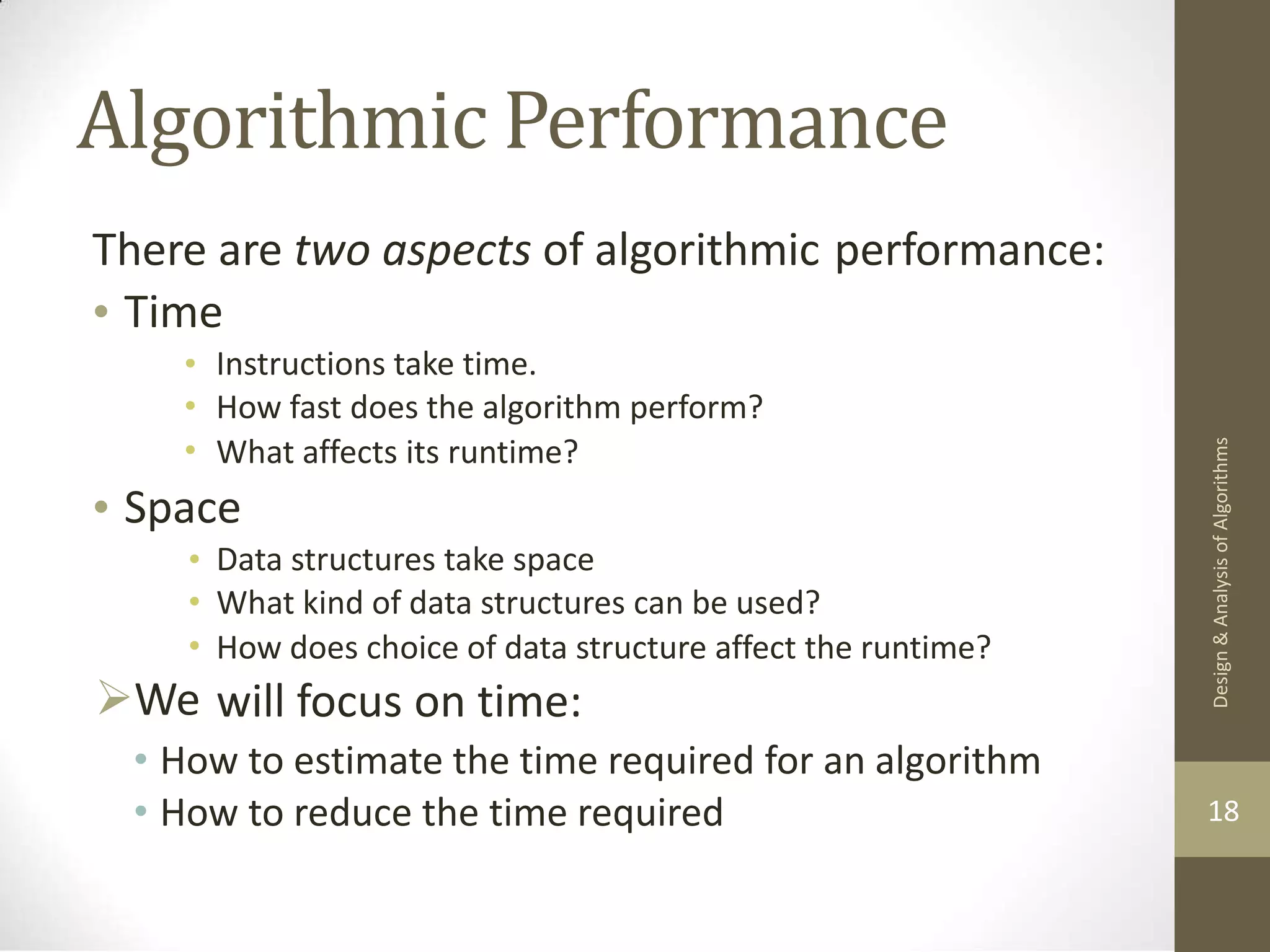
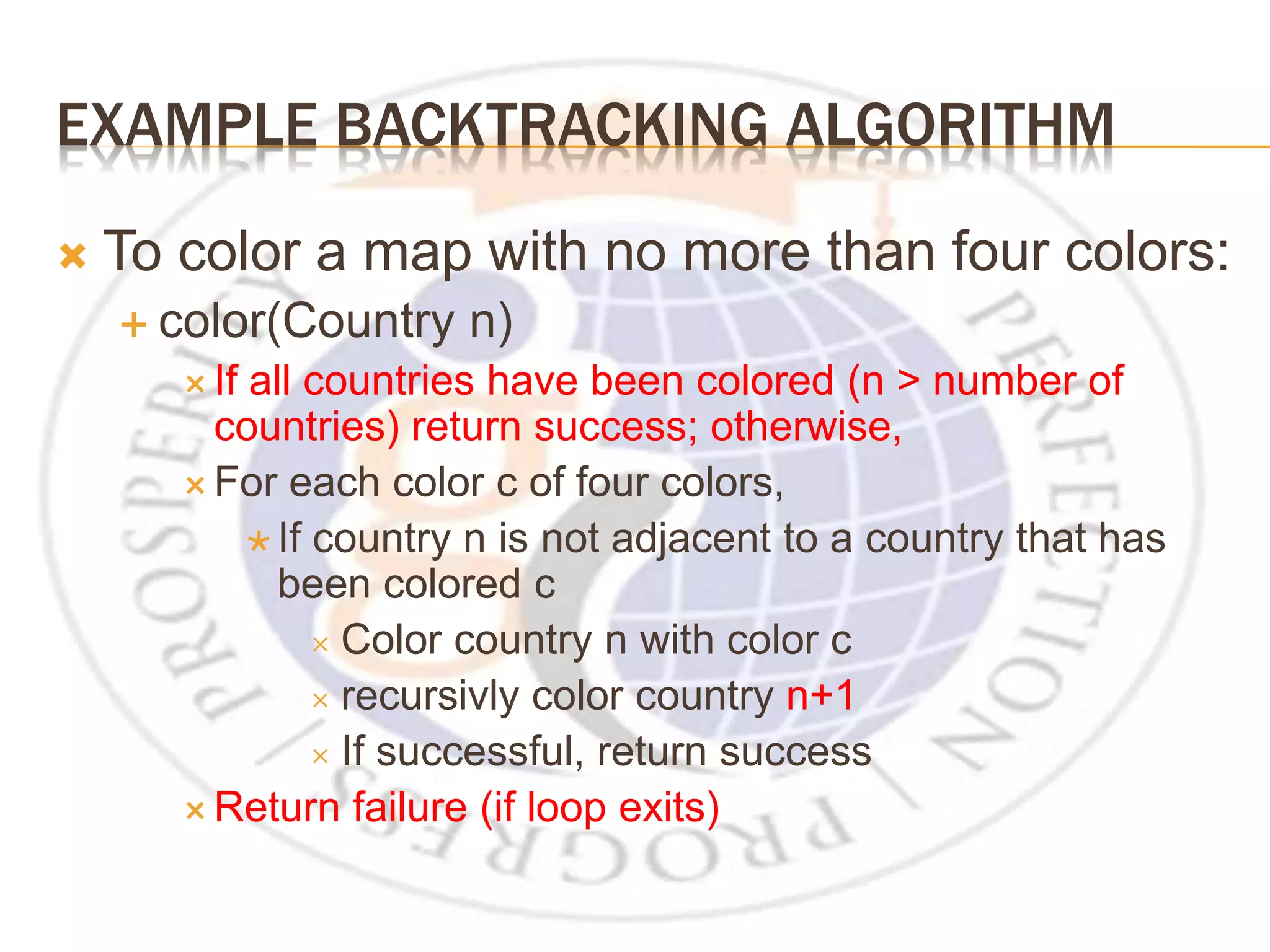
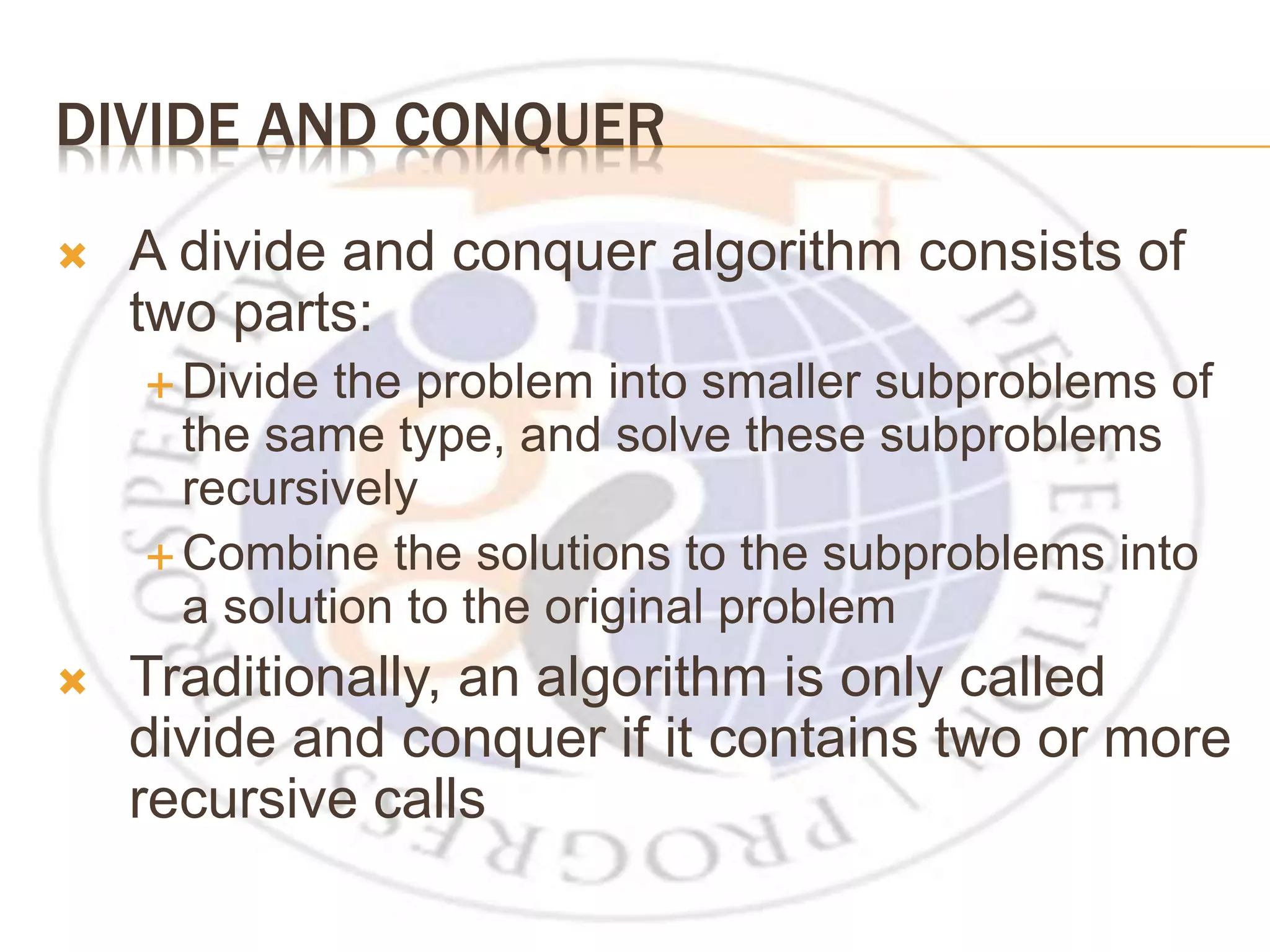
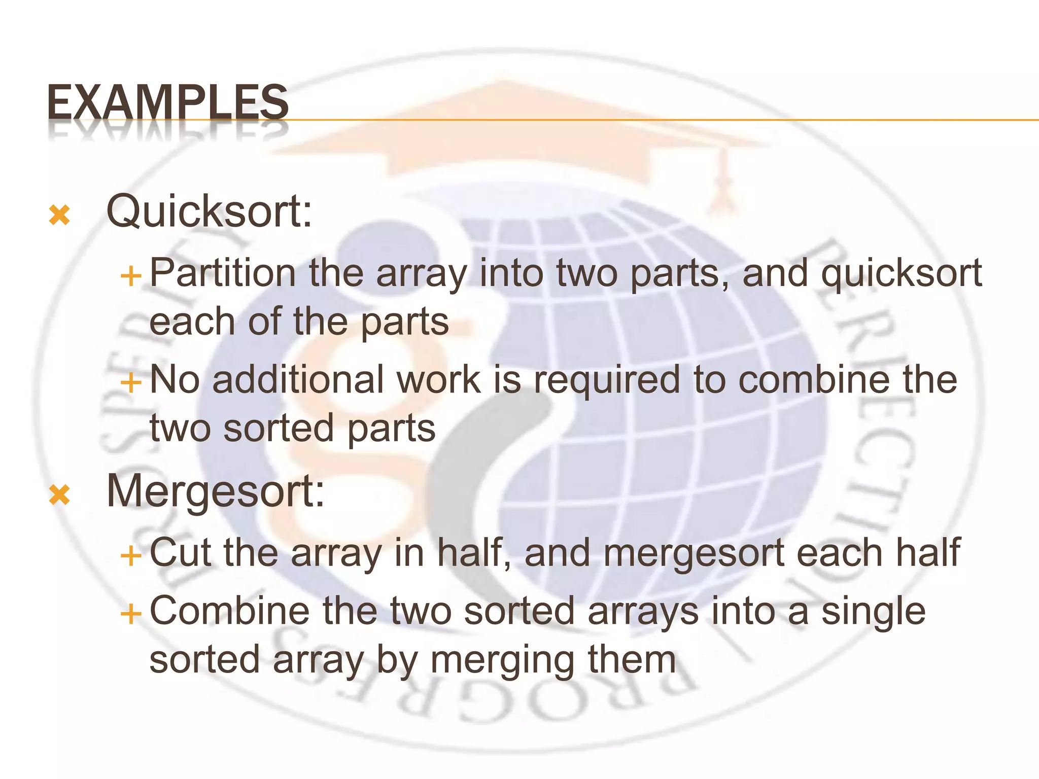
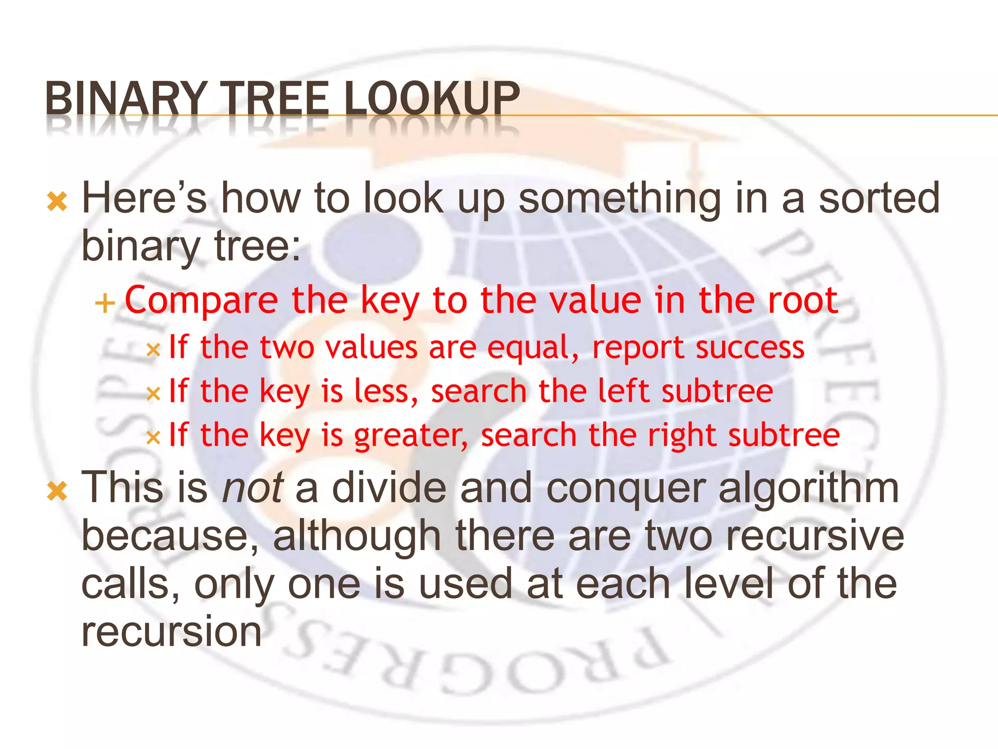
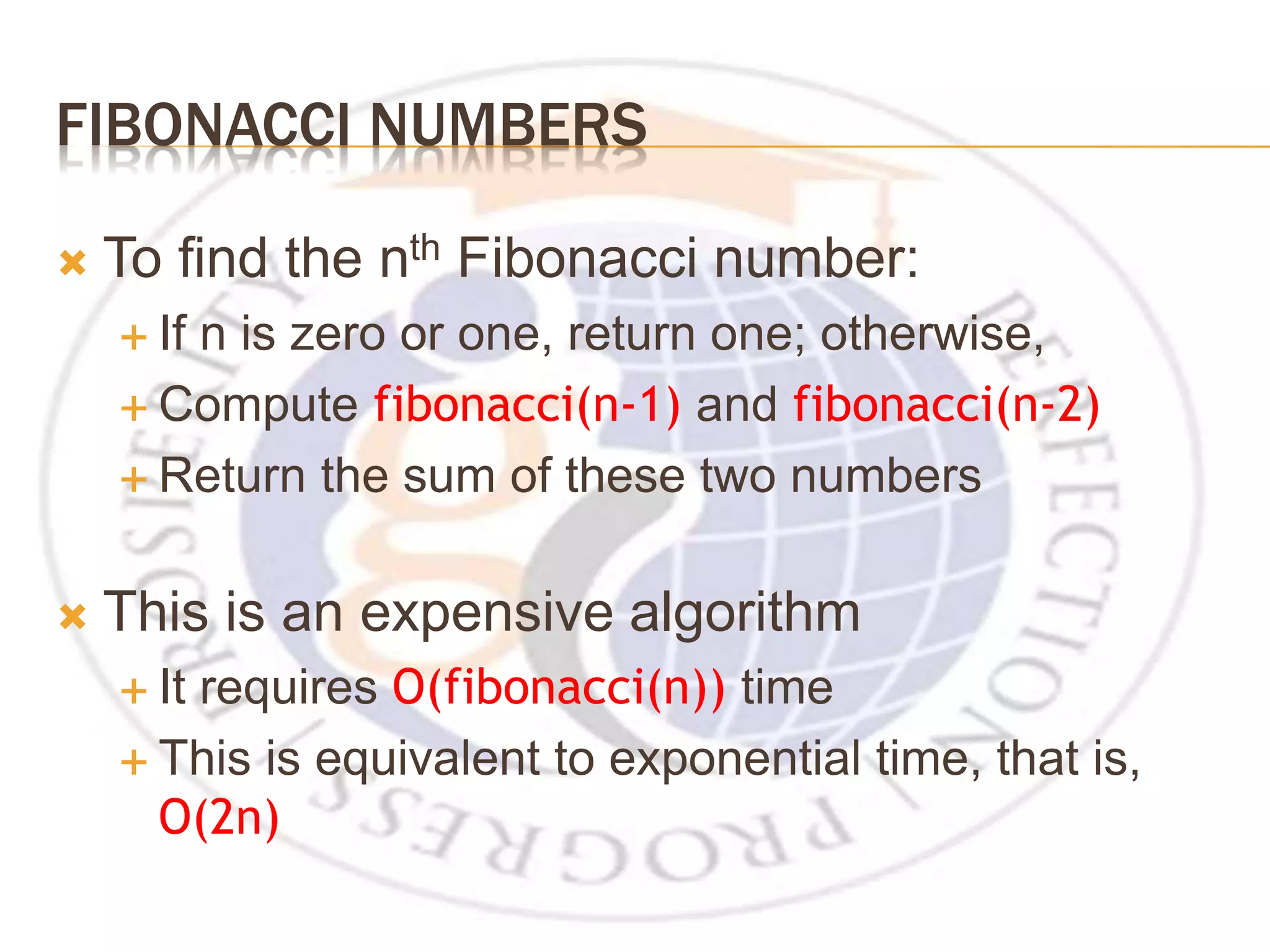
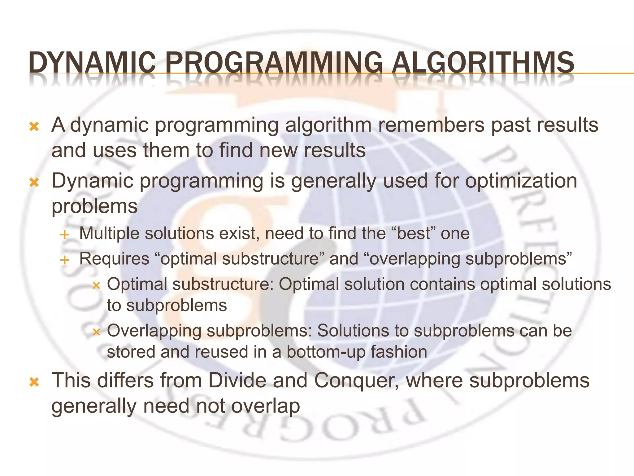
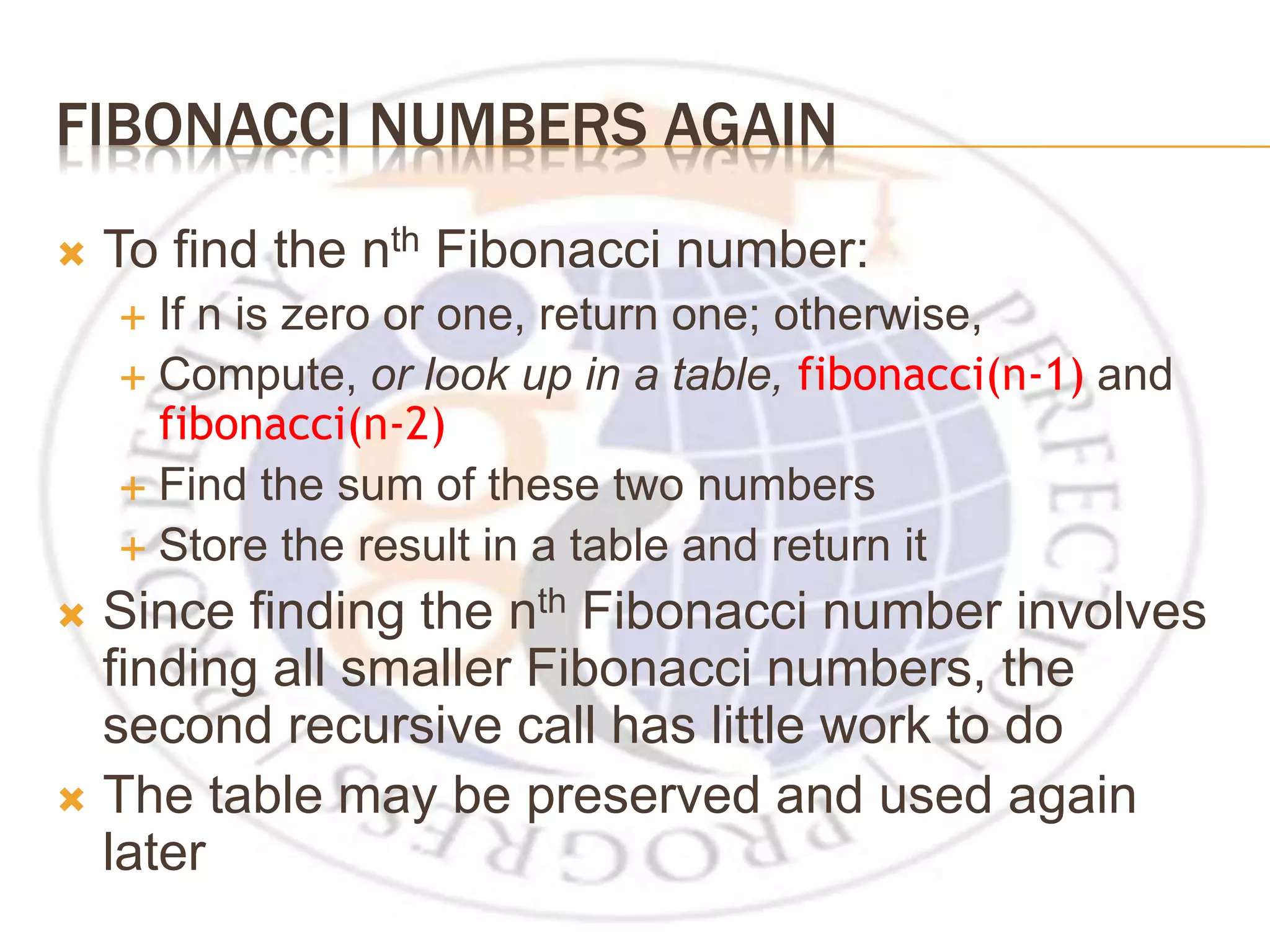
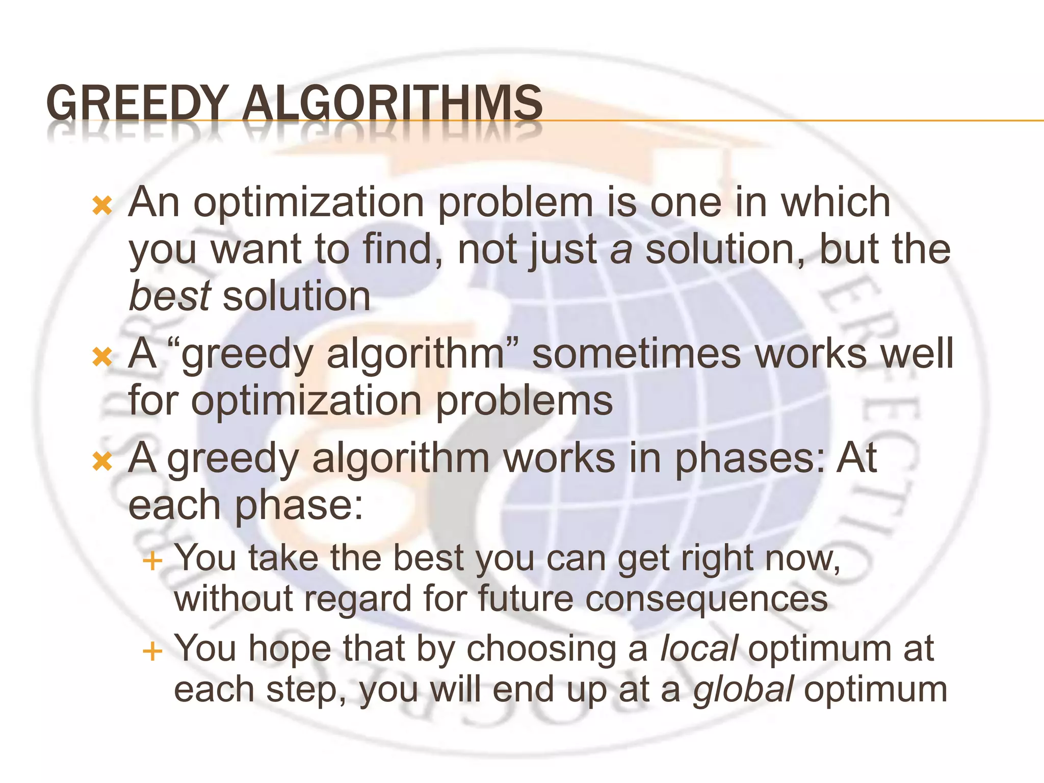
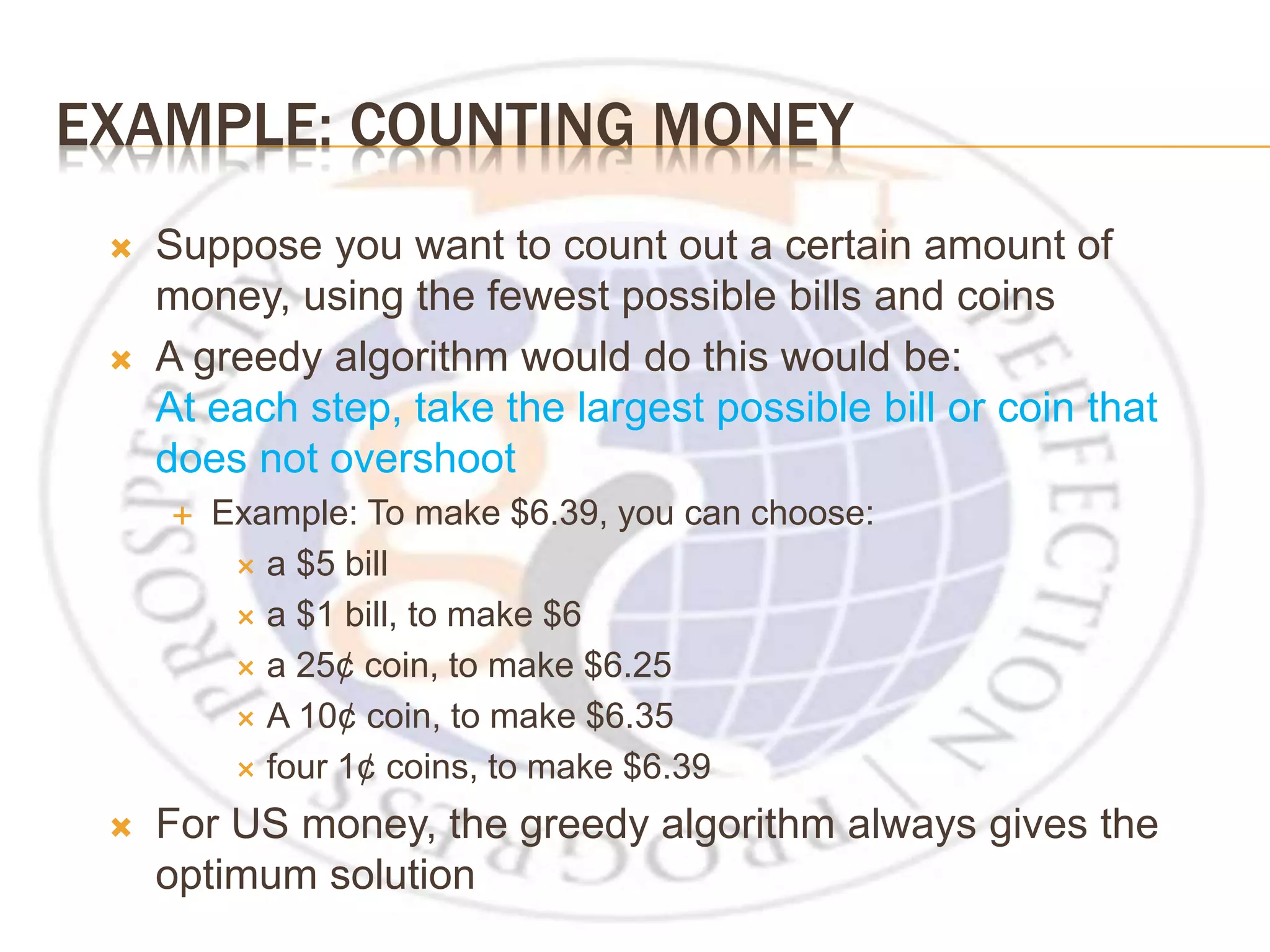
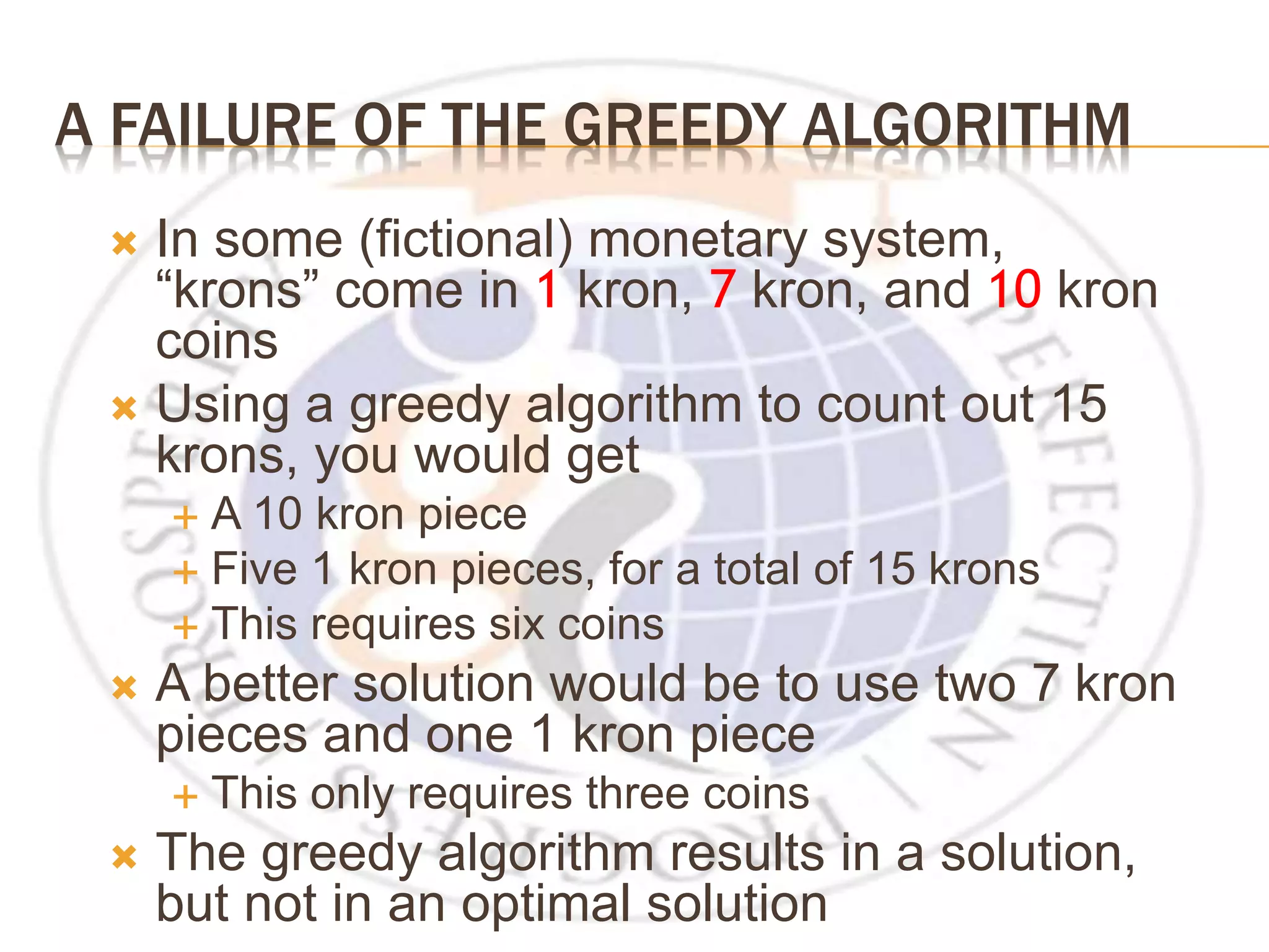
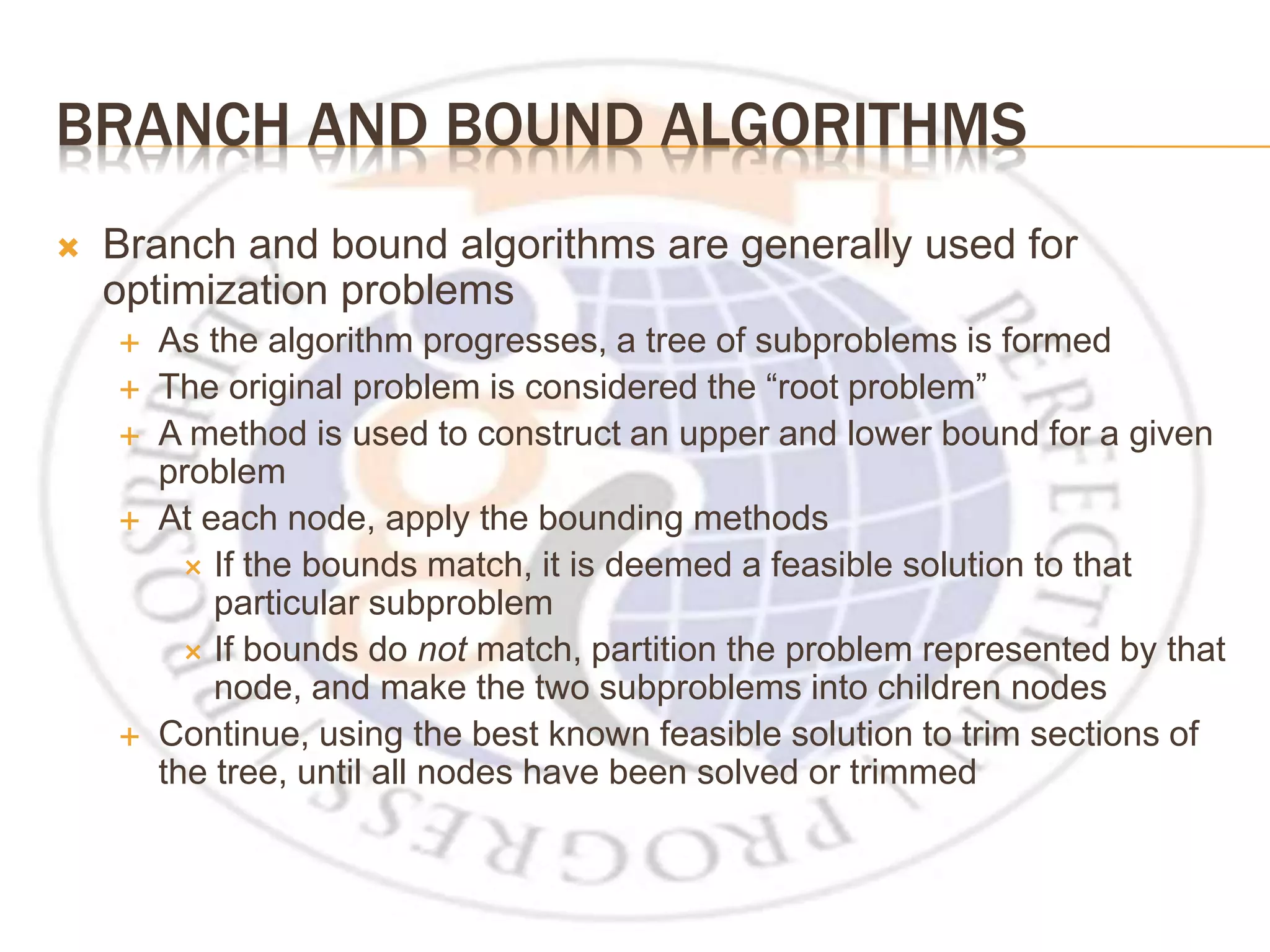
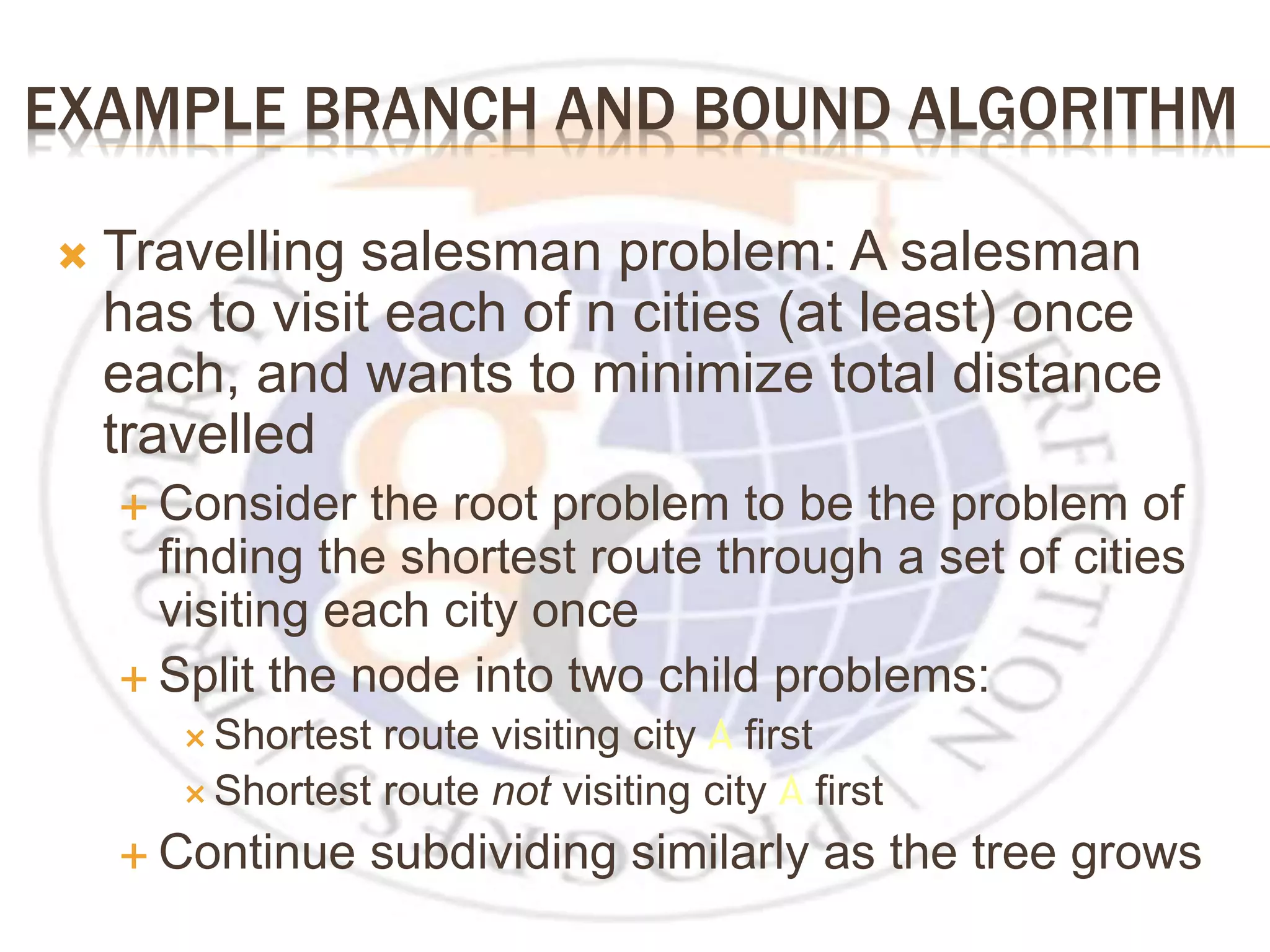
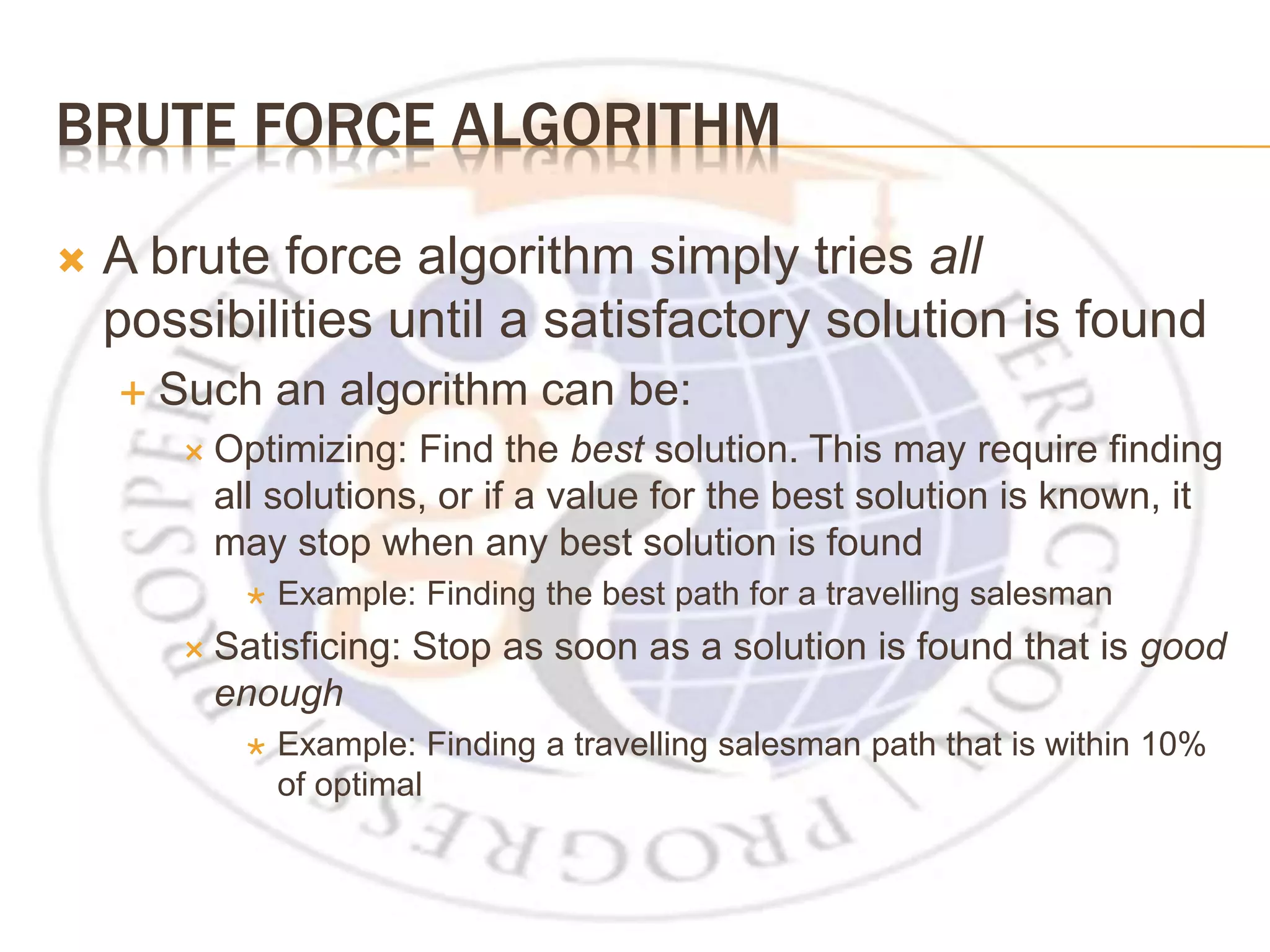
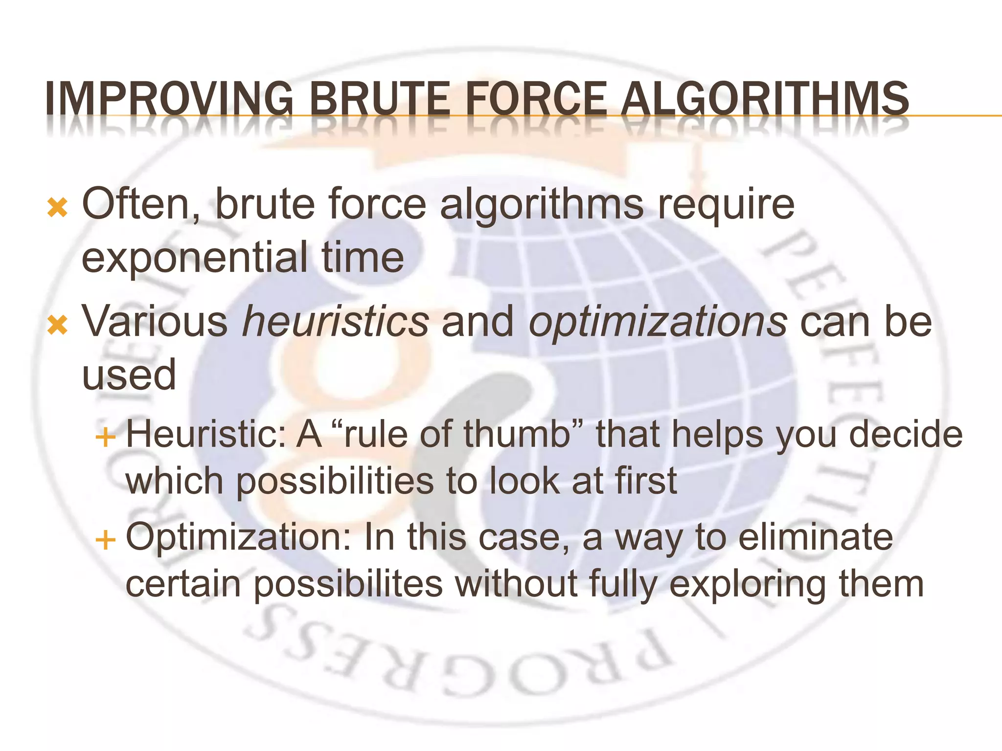
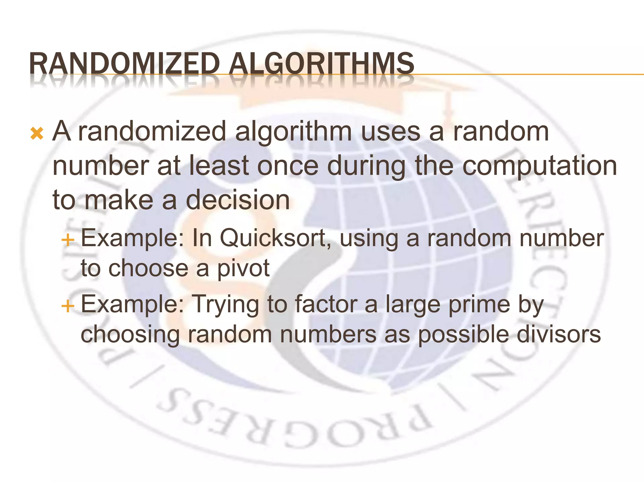
INTRODUCTION OF ALGORITHMS
COURSE  Course Code:  Course Title: Design and Analysis of Algorithm  Instructor: Ali Zaib Khan  Email Address: alizaib269@gmail.com  Term (Semester): Spring 2020  Duration: 15/16 Weeks
PROFILE & COORDINATES  Profile:  Name: Ali Zaib Khan  M.Phil (Computer Science) Minhaj University Lahore (MUL)  Bs (Software Engineering) Government College University Faisalabad (GCUF)  RESEARCH :Thesis  Enhancement in medical Field using Artificial Intelligence  Projects: Motion Sensor Camera Using MATLAB  Coordinates:  Email: alizaib269@gmail.com 3
Course Contents • • • • • • • • • • • • • • • Algorithm analysis Algorithm design Divide-and-conquer Greedy approach Graph algorithms Graph searching Topological sort approach Minimum spanning tree Shortest paths Backtracking and its applications in games. String matching. Longest common subsequence. Theory of NP-completeness. 7 Design & Analysis of Algorithms
Text Books • Course Book • Introduction to Algorithms, 3rd edition by Cormen, Leisersen, Rivest and Stein. • Reference Books • The Algorithm Design Manual - Steven S. • Algorithms – Dasgupta, Papadimitriou, Vazirani • Some relevant important material from internet as well 8 Design & Analysis of Algorithms
Advance Algorithm Analysis Lecture # 1 11 Design & Analysis of Algorithms
who invented algorithm Algorithms have a long history and the word can be traced back to the 9th century. At this time the Persian scientist, astronomer and mathematician Abdullah Muhammad bin Musa al-Khwarizmi, often cited as “The father of Algebra”, was indirect responsible for the creation of the term “Algorithm”.
Algorithms are the ideas behind computer programs. • An algorithm is an exact specification of how to solve a computational problem • An algorithm must specify every step completely, so a computer can implement it without any further “understanding” • An algorithm must work for all possible inputs of the problem. • Algorithms must be:  Correct: For each input produce an appropriate output  Efficient: run as quickly as possible, and use as little memory as possible – more about this later • There can be many different algorithms for each computational problem. Introduction
Introduction • An algorithm is a set of instructions to be followed to solve a problem. Another word, an algorithm is a complete set of rules that transform the input into the output in a finite number of steps. • There can be more than one solution (more than one algorithm) to solve a given problem. • An algorithm can be implemented using different programming languages on different platforms. • An algorithm should correctly solve the problem. • e.g., for sorting, this means even if (1) the input is already sorted, or (2) it contains repeated elements. • Once we have a correct algorithm for a problem, we have to determine the efficiency of that algorithm. 13 Design & Analysis of Algorithms
Design & Analysis of Algorithms Aspects of studying algorithms: 1. Designing algorithms: • • • putting the pieces of the puzzles together, choosing data structures, selecting the basic approaches to the solution of the problem, • The most popular design strategies are divide&conquer,greedy, dynamic prog., backtracking, and branch&bound. 2. Expressing and implementing the algorithm Concerns are: • • • • clearness conciseness Effectiveness etc. 15 Design & Analysis of Algorithms
Design & Analysis of Algorithms 3. Analyzing the algorithm Algorithm analysis is assessing the time and space resources required by an algorithm as a function of the size of the problem, without actually implementing the algorithm. 4. Compare enough UB and LB to see if your solution is good Analyzing the algorithm gives us the problem Analyzing the problem gives us the problem upper bound to solve the lower bound to solve the 5. Validate the algorithm We show that the algorithm computes possible legal (or given) inputs the correct answer for all 16 Design & Analysis of Algorithms
Design & Analysis of Algorithms 6. Verifying the algorithm (or program) An algorithm is said to be correct (verified) if, for every input instance, it halts with the correct output. 7. Testing algorithms There are two phases;  Debugging: The process of executing programs on sample data sets to determine if faulty results occur, and if so, to correct them. “Debugging can only point to the presence of errors, but not to their absence”  Profiling: the process of executing a correct program on 17 various data sets and measuring the time (and space) it takes to compute the results. Design & Analysis of Algorithms
Algorithmic Performance There are two aspects of algorithmic performance: • Time • • • Instructions take time. How fast does the algorithm perform? What affects its runtime? • Space • • • We Data structures take space What kind of data structures can be used? How does choice of data structure affect the runtime? will focus on time: • How to estimate the time required for an algorithm • How to reduce the time required 18 Design & Analysis of Algorithms
Algorithmic Analysis • Analysis of Algorithms is the area of computer science that provides tools to analyze the efficiency of different methods of solutions. • How do we compare the time efficiency of algorithms that solve the same problem? two Naïve Approach: implement these algorithms in a programming language (i.e., C++), and run them to compare their time requirements. 19 Design & Analysis of Algorithms
 Types of Algorithms
ALGORITHM CLASSIFICATION  Algorithms that use a similar problem- solving approach can be grouped together  This classification scheme is neither exhaustive nor disjoint  The purpose is not to be able to classify an algorithm as one type or another, but to highlight the various ways in which a problem can be attacked.
A SHORT LIST OF CATEGORIES  Algorithm types we will consider include:  Simple recursive algorithms  Backtracking algorithms  Divide and conquer algorithms  Dynamic programming algorithms  Greedy algorithms  Branch and bound algorithms  Brute force algorithms  Randomized algorithms
SIMPLE RECURSIVE ALGORITHMS I  A simple recursive algorithm:  Solves the base cases directly  recurs with a simpler subproblem  Does some extra work to convert the solution to the simpler subproblem into a solution to the given problem  We call these “simple” because several of the other algorithm types are inherently recursive
EXAMPLE RECURSIVE ALGORITHMS  To count the number of elements in a list:  If the list is empty, return zero; otherwise,  Step past the first element, and count the remaining elements in the list  Add one to the result  To test if a value occurs in a list:  If the list is empty, return false; otherwise,  If the first thing in the list is the given value, return true; otherwise  Step past the first element, and test whether the value occurs in the remainder of the list
BACKTRACKING ALGORITHMS  Backtracking algorithms are based on a depth-first recursive search  A backtracking algorithm:  Tests to see if a solution has been found, and if so, returns it; otherwise  For each choice that can be made at this point,  Make that choice  Recur  If the recursion returns a solution, return it  If no choices remain, return failure
EXAMPLE BACKTRACKING ALGORITHM  To color a map with no more than four colors:  color(Country n)  If all countries have been colored (n > number of countries) return success; otherwise,  For each color c of four colors,  If country n is not adjacent to a country that has been colored c  Color country n with color c  recursivly color country n+1  If successful, return success  Return failure (if loop exits)
DIVIDE AND CONQUER  A divide and conquer algorithm consists of two parts:  Divide the problem into smaller subproblems of the same type, and solve these subproblems recursively  Combine the solutions to the subproblems into a solution to the original problem  Traditionally, an algorithm is only called divide and conquer if it contains two or more recursive calls
EXAMPLES  Quicksort:  Partition the array into two parts, and quicksort each of the parts  No additional work is required to combine the two sorted parts  Mergesort:  Cut the array in half, and mergesort each half  Combine the two sorted arrays into a single sorted array by merging them
BINARY TREE LOOKUP  Here’s how to look up something in a sorted binary tree:  Compare the key to the value in the root  If the two values are equal, report success  If the key is less, search the left subtree  If the key is greater, search the right subtree  This is not a divide and conquer algorithm because, although there are two recursive calls, only one is used at each level of the recursion
FIBONACCI NUMBERS  To find the nth Fibonacci number:  If n is zero or one, return one; otherwise,  Compute fibonacci(n-1) and fibonacci(n-2)  Return the sum of these two numbers  This is an expensive algorithm  It requires O(fibonacci(n)) time  This is equivalent to exponential time, that is, O(2n)
DYNAMIC PROGRAMMING ALGORITHMS  A dynamic programming algorithm remembers past results and uses them to find new results  Dynamic programming is generally used for optimization problems  Multiple solutions exist, need to find the “best” one  Requires “optimal substructure” and “overlapping subproblems”  Optimal substructure: Optimal solution contains optimal solutions to subproblems  Overlapping subproblems: Solutions to subproblems can be stored and reused in a bottom-up fashion  This differs from Divide and Conquer, where subproblems generally need not overlap
FIBONACCI NUMBERS AGAIN  To find the nth Fibonacci number:  If n is zero or one, return one; otherwise,  Compute, or look up in a table, fibonacci(n-1) and fibonacci(n-2)  Find the sum of these two numbers  Store the result in a table and return it  Since finding the nth Fibonacci number involves finding all smaller Fibonacci numbers, the second recursive call has little work to do  The table may be preserved and used again later
GREEDY ALGORITHMS  An optimization problem is one in which you want to find, not just a solution, but the best solution  A “greedy algorithm” sometimes works well for optimization problems  A greedy algorithm works in phases: At each phase:  You take the best you can get right now, without regard for future consequences  You hope that by choosing a local optimum at each step, you will end up at a global optimum
EXAMPLE: COUNTING MONEY  Suppose you want to count out a certain amount of money, using the fewest possible bills and coins  A greedy algorithm would do this would be: At each step, take the largest possible bill or coin that does not overshoot  Example: To make $6.39, you can choose:  a $5 bill  a $1 bill, to make $6  a 25¢ coin, to make $6.25  A 10¢ coin, to make $6.35  four 1¢ coins, to make $6.39  For US money, the greedy algorithm always gives the optimum solution
A FAILURE OF THE GREEDY ALGORITHM  In some (fictional) monetary system, “krons” come in 1 kron, 7 kron, and 10 kron coins  Using a greedy algorithm to count out 15 krons, you would get  A 10 kron piece  Five 1 kron pieces, for a total of 15 krons  This requires six coins  A better solution would be to use two 7 kron pieces and one 1 kron piece  This only requires three coins  The greedy algorithm results in a solution, but not in an optimal solution
BRANCH AND BOUND ALGORITHMS  Branch and bound algorithms are generally used for optimization problems  As the algorithm progresses, a tree of subproblems is formed  The original problem is considered the “root problem”  A method is used to construct an upper and lower bound for a given problem  At each node, apply the bounding methods  If the bounds match, it is deemed a feasible solution to that particular subproblem  If bounds do not match, partition the problem represented by that node, and make the two subproblems into children nodes  Continue, using the best known feasible solution to trim sections of the tree, until all nodes have been solved or trimmed
EXAMPLE BRANCH AND BOUND ALGORITHM  Travelling salesman problem: A salesman has to visit each of n cities (at least) once each, and wants to minimize total distance travelled  Consider the root problem to be the problem of finding the shortest route through a set of cities visiting each city once  Split the node into two child problems:  Shortest route visiting city A first  Shortest route not visiting city A first  Continue subdividing similarly as the tree grows
BRUTE FORCE ALGORITHM  A brute force algorithm simply tries all possibilities until a satisfactory solution is found  Such an algorithm can be:  Optimizing: Find the best solution. This may require finding all solutions, or if a value for the best solution is known, it may stop when any best solution is found  Example: Finding the best path for a travelling salesman  Satisficing: Stop as soon as a solution is found that is good enough  Example: Finding a travelling salesman path that is within 10% of optimal
IMPROVING BRUTE FORCE ALGORITHMS  Often, brute force algorithms require exponential time  Various heuristics and optimizations can be used  Heuristic: A “rule of thumb” that helps you decide which possibilities to look at first  Optimization: In this case, a way to eliminate certain possibilites without fully exploring them
RANDOMIZED ALGORITHMS  A randomized algorithm uses a random number at least once during the computation to make a decision  Example: In Quicksort, using a random number to choose a pivot  Example: Trying to factor a large prime by choosing random numbers as possible divisors
THE END

Types of Algorithms.ppt

  • 1.
  • 2.
    COURSE  Course Code: Course Title: Design and Analysis of Algorithm  Instructor: Ali Zaib Khan  Email Address: alizaib269@gmail.com  Term (Semester): Spring 2020  Duration: 15/16 Weeks
  • 3.
    PROFILE & COORDINATES Profile:  Name: Ali Zaib Khan  M.Phil (Computer Science) Minhaj University Lahore (MUL)  Bs (Software Engineering) Government College University Faisalabad (GCUF)  RESEARCH :Thesis  Enhancement in medical Field using Artificial Intelligence  Projects: Motion Sensor Camera Using MATLAB  Coordinates:  Email: alizaib269@gmail.com 3
  • 4.
    Course Contents • • • • • • • • • • • • • • • Algorithm analysis Algorithmdesign Divide-and-conquer Greedy approach Graph algorithms Graph searching Topological sort approach Minimum spanning tree Shortest paths Backtracking and its applications in games. String matching. Longest common subsequence. Theory of NP-completeness. 7 Design & Analysis of Algorithms
  • 5.
    Text Books • CourseBook • Introduction to Algorithms, 3rd edition by Cormen, Leisersen, Rivest and Stein. • Reference Books • The Algorithm Design Manual - Steven S. • Algorithms – Dasgupta, Papadimitriou, Vazirani • Some relevant important material from internet as well 8 Design & Analysis of Algorithms
  • 6.
    Advance Algorithm Analysis Lecture# 1 11 Design & Analysis of Algorithms
  • 7.
    who invented algorithm Algorithmshave a long history and the word can be traced back to the 9th century. At this time the Persian scientist, astronomer and mathematician Abdullah Muhammad bin Musa al-Khwarizmi, often cited as “The father of Algebra”, was indirect responsible for the creation of the term “Algorithm”.
  • 8.
    Algorithms are theideas behind computer programs. • An algorithm is an exact specification of how to solve a computational problem • An algorithm must specify every step completely, so a computer can implement it without any further “understanding” • An algorithm must work for all possible inputs of the problem. • Algorithms must be:  Correct: For each input produce an appropriate output  Efficient: run as quickly as possible, and use as little memory as possible – more about this later • There can be many different algorithms for each computational problem. Introduction
  • 9.
    Introduction • An algorithmis a set of instructions to be followed to solve a problem. Another word, an algorithm is a complete set of rules that transform the input into the output in a finite number of steps. • There can be more than one solution (more than one algorithm) to solve a given problem. • An algorithm can be implemented using different programming languages on different platforms. • An algorithm should correctly solve the problem. • e.g., for sorting, this means even if (1) the input is already sorted, or (2) it contains repeated elements. • Once we have a correct algorithm for a problem, we have to determine the efficiency of that algorithm. 13 Design & Analysis of Algorithms
  • 10.
    Design & Analysisof Algorithms Aspects of studying algorithms: 1. Designing algorithms: • • • putting the pieces of the puzzles together, choosing data structures, selecting the basic approaches to the solution of the problem, • The most popular design strategies are divide&conquer,greedy, dynamic prog., backtracking, and branch&bound. 2. Expressing and implementing the algorithm Concerns are: • • • • clearness conciseness Effectiveness etc. 15 Design & Analysis of Algorithms
  • 11.
    Design & Analysisof Algorithms 3. Analyzing the algorithm Algorithm analysis is assessing the time and space resources required by an algorithm as a function of the size of the problem, without actually implementing the algorithm. 4. Compare enough UB and LB to see if your solution is good Analyzing the algorithm gives us the problem Analyzing the problem gives us the problem upper bound to solve the lower bound to solve the 5. Validate the algorithm We show that the algorithm computes possible legal (or given) inputs the correct answer for all 16 Design & Analysis of Algorithms
  • 12.
    Design & Analysisof Algorithms 6. Verifying the algorithm (or program) An algorithm is said to be correct (verified) if, for every input instance, it halts with the correct output. 7. Testing algorithms There are two phases;  Debugging: The process of executing programs on sample data sets to determine if faulty results occur, and if so, to correct them. “Debugging can only point to the presence of errors, but not to their absence”  Profiling: the process of executing a correct program on 17 various data sets and measuring the time (and space) it takes to compute the results. Design & Analysis of Algorithms
  • 13.
    Algorithmic Performance There aretwo aspects of algorithmic performance: • Time • • • Instructions take time. How fast does the algorithm perform? What affects its runtime? • Space • • • We Data structures take space What kind of data structures can be used? How does choice of data structure affect the runtime? will focus on time: • How to estimate the time required for an algorithm • How to reduce the time required 18 Design & Analysis of Algorithms
  • 14.
    Algorithmic Analysis • Analysisof Algorithms is the area of computer science that provides tools to analyze the efficiency of different methods of solutions. • How do we compare the time efficiency of algorithms that solve the same problem? two Naïve Approach: implement these algorithms in a programming language (i.e., C++), and run them to compare their time requirements. 19 Design & Analysis of Algorithms
  • 15.
     Types ofAlgorithms
  • 16.
    ALGORITHM CLASSIFICATION  Algorithmsthat use a similar problem- solving approach can be grouped together  This classification scheme is neither exhaustive nor disjoint  The purpose is not to be able to classify an algorithm as one type or another, but to highlight the various ways in which a problem can be attacked.
  • 17.
    A SHORT LISTOF CATEGORIES  Algorithm types we will consider include:  Simple recursive algorithms  Backtracking algorithms  Divide and conquer algorithms  Dynamic programming algorithms  Greedy algorithms  Branch and bound algorithms  Brute force algorithms  Randomized algorithms
  • 18.
    SIMPLE RECURSIVE ALGORITHMSI  A simple recursive algorithm:  Solves the base cases directly  recurs with a simpler subproblem  Does some extra work to convert the solution to the simpler subproblem into a solution to the given problem  We call these “simple” because several of the other algorithm types are inherently recursive
  • 19.
    EXAMPLE RECURSIVE ALGORITHMS To count the number of elements in a list:  If the list is empty, return zero; otherwise,  Step past the first element, and count the remaining elements in the list  Add one to the result  To test if a value occurs in a list:  If the list is empty, return false; otherwise,  If the first thing in the list is the given value, return true; otherwise  Step past the first element, and test whether the value occurs in the remainder of the list
  • 20.
    BACKTRACKING ALGORITHMS  Backtrackingalgorithms are based on a depth-first recursive search  A backtracking algorithm:  Tests to see if a solution has been found, and if so, returns it; otherwise  For each choice that can be made at this point,  Make that choice  Recur  If the recursion returns a solution, return it  If no choices remain, return failure
  • 21.
    EXAMPLE BACKTRACKING ALGORITHM To color a map with no more than four colors:  color(Country n)  If all countries have been colored (n > number of countries) return success; otherwise,  For each color c of four colors,  If country n is not adjacent to a country that has been colored c  Color country n with color c  recursivly color country n+1  If successful, return success  Return failure (if loop exits)
  • 22.
    DIVIDE AND CONQUER A divide and conquer algorithm consists of two parts:  Divide the problem into smaller subproblems of the same type, and solve these subproblems recursively  Combine the solutions to the subproblems into a solution to the original problem  Traditionally, an algorithm is only called divide and conquer if it contains two or more recursive calls
  • 23.
    EXAMPLES  Quicksort:  Partitionthe array into two parts, and quicksort each of the parts  No additional work is required to combine the two sorted parts  Mergesort:  Cut the array in half, and mergesort each half  Combine the two sorted arrays into a single sorted array by merging them
  • 24.
    BINARY TREE LOOKUP Here’s how to look up something in a sorted binary tree:  Compare the key to the value in the root  If the two values are equal, report success  If the key is less, search the left subtree  If the key is greater, search the right subtree  This is not a divide and conquer algorithm because, although there are two recursive calls, only one is used at each level of the recursion
  • 25.
    FIBONACCI NUMBERS  Tofind the nth Fibonacci number:  If n is zero or one, return one; otherwise,  Compute fibonacci(n-1) and fibonacci(n-2)  Return the sum of these two numbers  This is an expensive algorithm  It requires O(fibonacci(n)) time  This is equivalent to exponential time, that is, O(2n)
  • 26.
    DYNAMIC PROGRAMMING ALGORITHMS A dynamic programming algorithm remembers past results and uses them to find new results  Dynamic programming is generally used for optimization problems  Multiple solutions exist, need to find the “best” one  Requires “optimal substructure” and “overlapping subproblems”  Optimal substructure: Optimal solution contains optimal solutions to subproblems  Overlapping subproblems: Solutions to subproblems can be stored and reused in a bottom-up fashion  This differs from Divide and Conquer, where subproblems generally need not overlap
  • 27.
    FIBONACCI NUMBERS AGAIN To find the nth Fibonacci number:  If n is zero or one, return one; otherwise,  Compute, or look up in a table, fibonacci(n-1) and fibonacci(n-2)  Find the sum of these two numbers  Store the result in a table and return it  Since finding the nth Fibonacci number involves finding all smaller Fibonacci numbers, the second recursive call has little work to do  The table may be preserved and used again later
  • 28.
    GREEDY ALGORITHMS  Anoptimization problem is one in which you want to find, not just a solution, but the best solution  A “greedy algorithm” sometimes works well for optimization problems  A greedy algorithm works in phases: At each phase:  You take the best you can get right now, without regard for future consequences  You hope that by choosing a local optimum at each step, you will end up at a global optimum
  • 29.
    EXAMPLE: COUNTING MONEY Suppose you want to count out a certain amount of money, using the fewest possible bills and coins  A greedy algorithm would do this would be: At each step, take the largest possible bill or coin that does not overshoot  Example: To make $6.39, you can choose:  a $5 bill  a $1 bill, to make $6  a 25¢ coin, to make $6.25  A 10¢ coin, to make $6.35  four 1¢ coins, to make $6.39  For US money, the greedy algorithm always gives the optimum solution
  • 30.
    A FAILURE OFTHE GREEDY ALGORITHM  In some (fictional) monetary system, “krons” come in 1 kron, 7 kron, and 10 kron coins  Using a greedy algorithm to count out 15 krons, you would get  A 10 kron piece  Five 1 kron pieces, for a total of 15 krons  This requires six coins  A better solution would be to use two 7 kron pieces and one 1 kron piece  This only requires three coins  The greedy algorithm results in a solution, but not in an optimal solution
  • 31.
    BRANCH AND BOUNDALGORITHMS  Branch and bound algorithms are generally used for optimization problems  As the algorithm progresses, a tree of subproblems is formed  The original problem is considered the “root problem”  A method is used to construct an upper and lower bound for a given problem  At each node, apply the bounding methods  If the bounds match, it is deemed a feasible solution to that particular subproblem  If bounds do not match, partition the problem represented by that node, and make the two subproblems into children nodes  Continue, using the best known feasible solution to trim sections of the tree, until all nodes have been solved or trimmed
  • 32.
    EXAMPLE BRANCH ANDBOUND ALGORITHM  Travelling salesman problem: A salesman has to visit each of n cities (at least) once each, and wants to minimize total distance travelled  Consider the root problem to be the problem of finding the shortest route through a set of cities visiting each city once  Split the node into two child problems:  Shortest route visiting city A first  Shortest route not visiting city A first  Continue subdividing similarly as the tree grows
  • 33.
    BRUTE FORCE ALGORITHM A brute force algorithm simply tries all possibilities until a satisfactory solution is found  Such an algorithm can be:  Optimizing: Find the best solution. This may require finding all solutions, or if a value for the best solution is known, it may stop when any best solution is found  Example: Finding the best path for a travelling salesman  Satisficing: Stop as soon as a solution is found that is good enough  Example: Finding a travelling salesman path that is within 10% of optimal
  • 34.
    IMPROVING BRUTE FORCEALGORITHMS  Often, brute force algorithms require exponential time  Various heuristics and optimizations can be used  Heuristic: A “rule of thumb” that helps you decide which possibilities to look at first  Optimization: In this case, a way to eliminate certain possibilites without fully exploring them
  • 35.
    RANDOMIZED ALGORITHMS  Arandomized algorithm uses a random number at least once during the computation to make a decision  Example: In Quicksort, using a random number to choose a pivot  Example: Trying to factor a large prime by choosing random numbers as possible divisors
  • 36.