
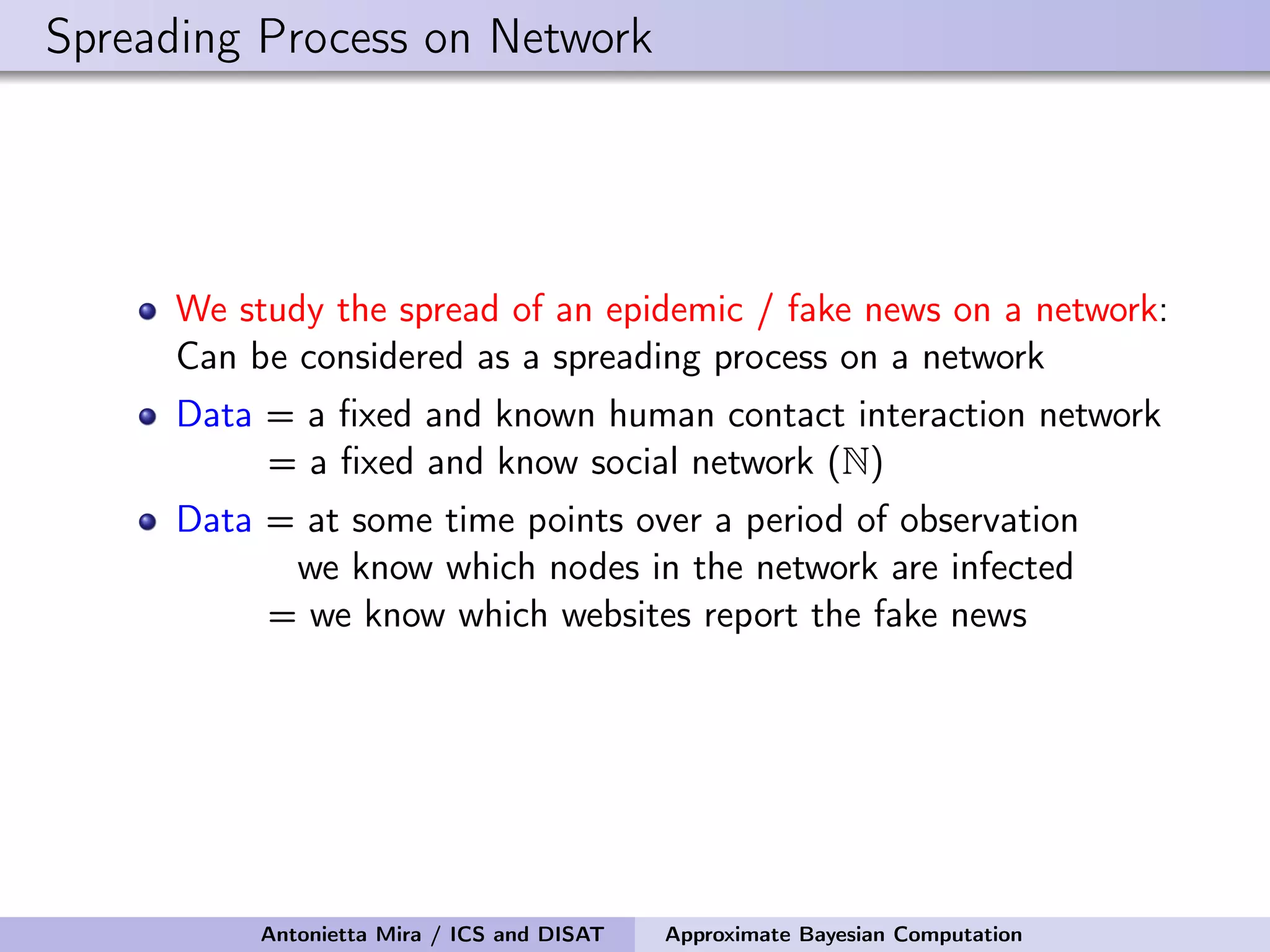
Download as PDF, PPTX

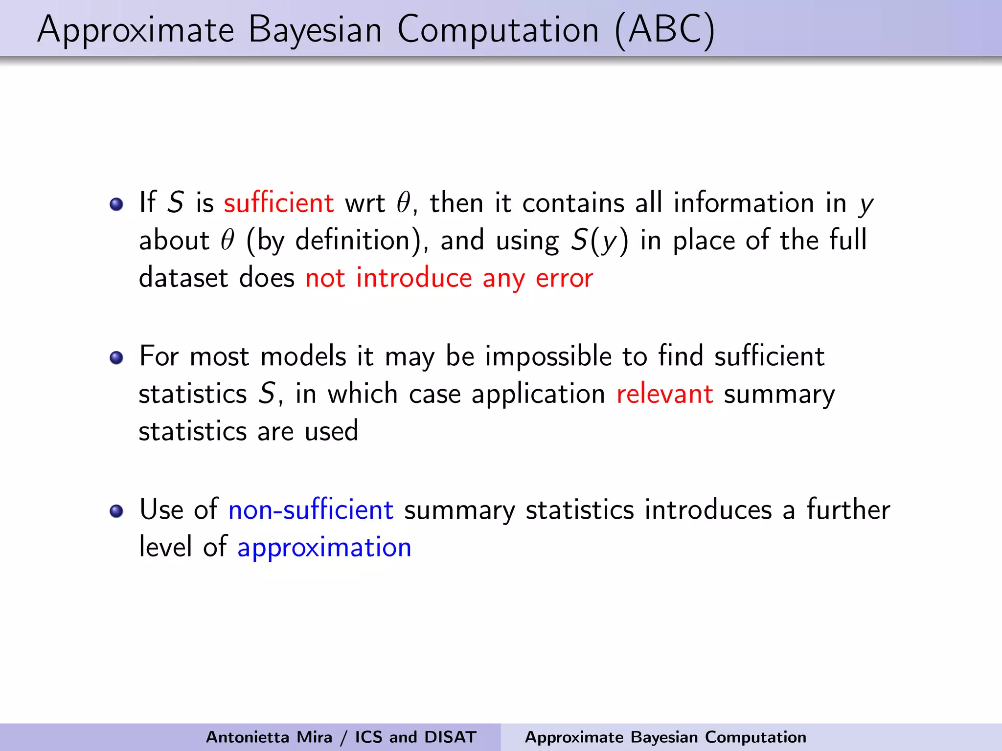
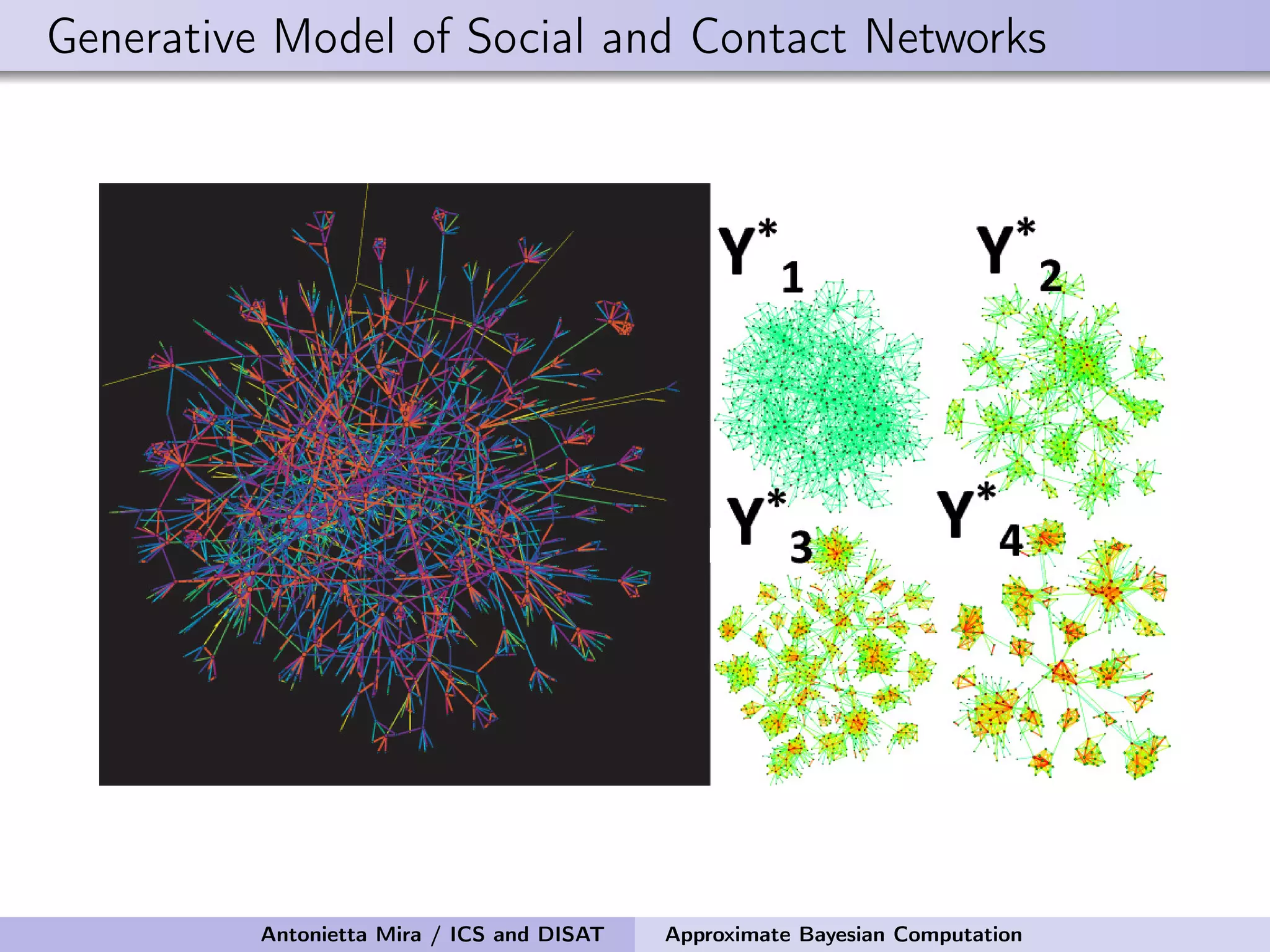
![Exact Bayesian inference for ER Beta prior p(θ) = Beta(α = 5, β = 50) Beta posterior p(θ|D) = Beta(α + L, β + [N(N − 1)/2) − L]) Bayesian Estimator = posterior mean Antonietta Mira / ICS and DISAT Approximate Bayesian Computation](https://image.slidesharecdn.com/mirasamsidec132017-171214220909/75/QMC-Program-Trends-and-Advances-in-Monte-Carlo-Sampling-Algorithms-Workshop-Approximate-Bayesian-Computation-for-Inference-in-Generative-Models-for-Large-scale-Network-Data-Antonietta-Mira-Dec-13-2017-29-2048.jpg)
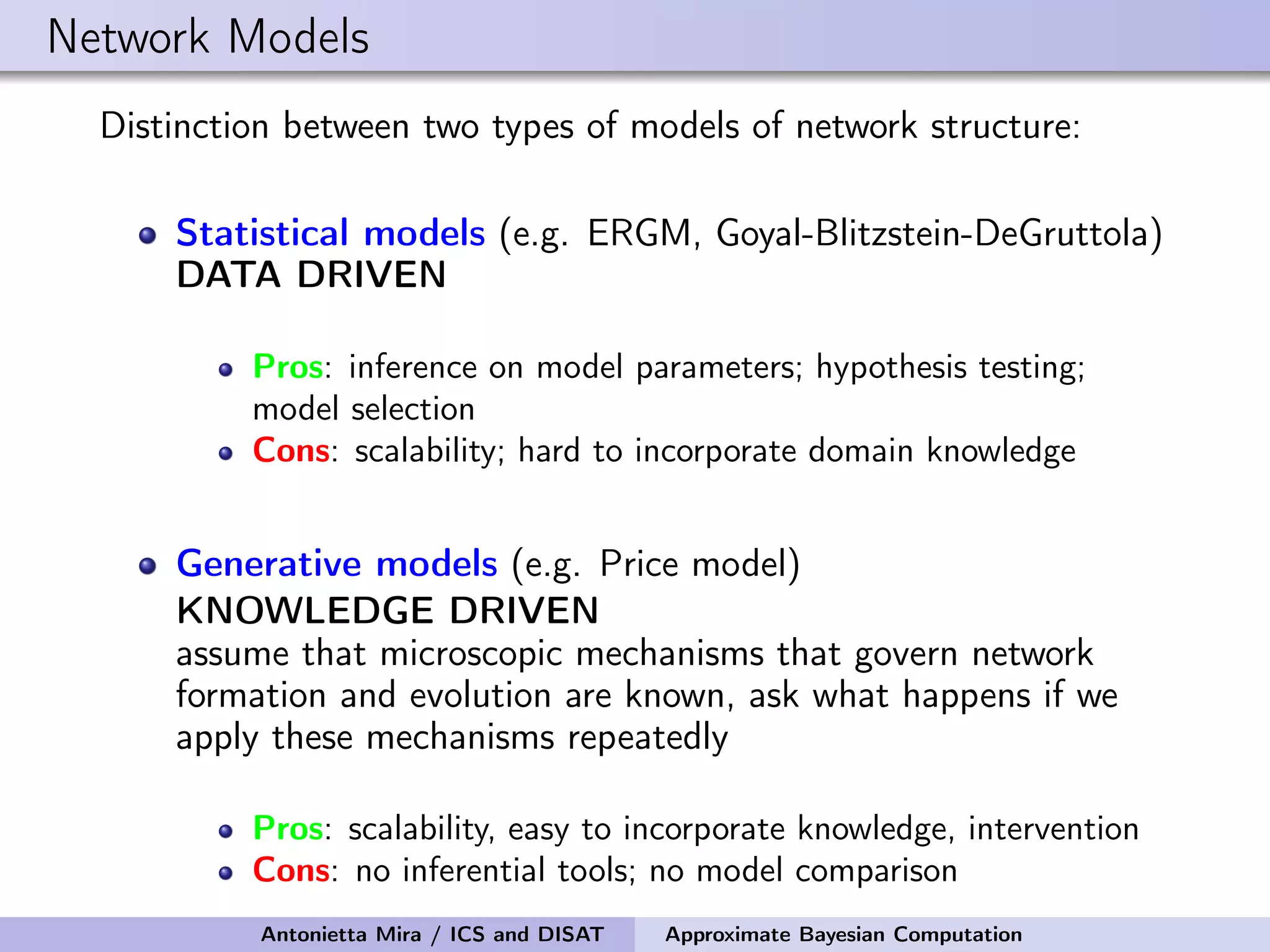
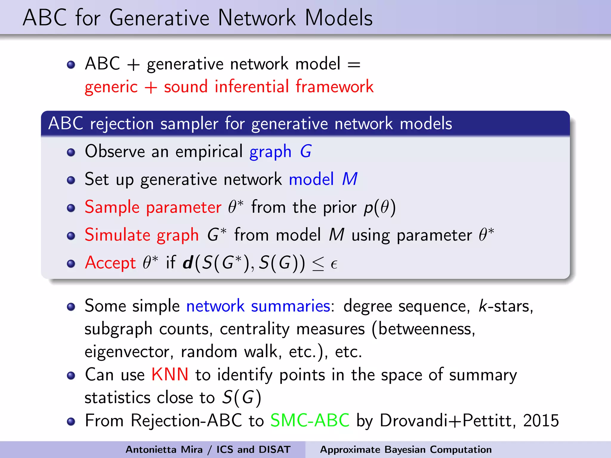
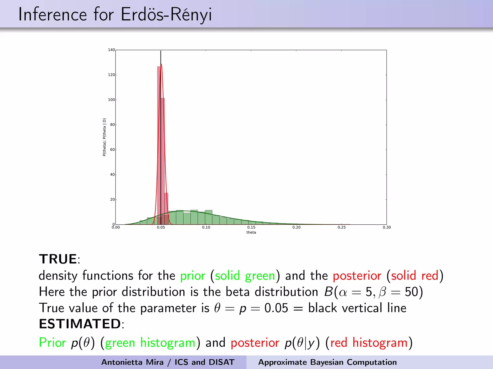
![Approximate Bayesian inference for Erdös-Rényi Simulate observed ER graph G from a model with N = 100 and p = 0.05 Number of edges = summary statistic = S(G) = L We perform 100,000 draws from the prior pi For each pi , we generate a sequence of graphs G1 i , . . . , GK i , compute corresponding summary statistics S(G1 i ), . . . , S(GK i ), retain pi if S(Gi ) = Li = L = S(G) We retained only 162 values of pi The mean and median of the prior are 0.091 and 0.086 the 95% prior credible interval is [0.031, 0.178] The mean and median of the posterior are 0.050 and 0.050 the 95% posterior credible interval is [0.043, 0.055] Antonietta Mira / ICS and DISAT Approximate Bayesian Computation](https://image.slidesharecdn.com/mirasamsidec132017-171214220909/75/QMC-Program-Trends-and-Advances-in-Monte-Carlo-Sampling-Algorithms-Workshop-Approximate-Bayesian-Computation-for-Inference-in-Generative-Models-for-Large-scale-Network-Data-Antonietta-Mira-Dec-13-2017-33-2048.jpg)
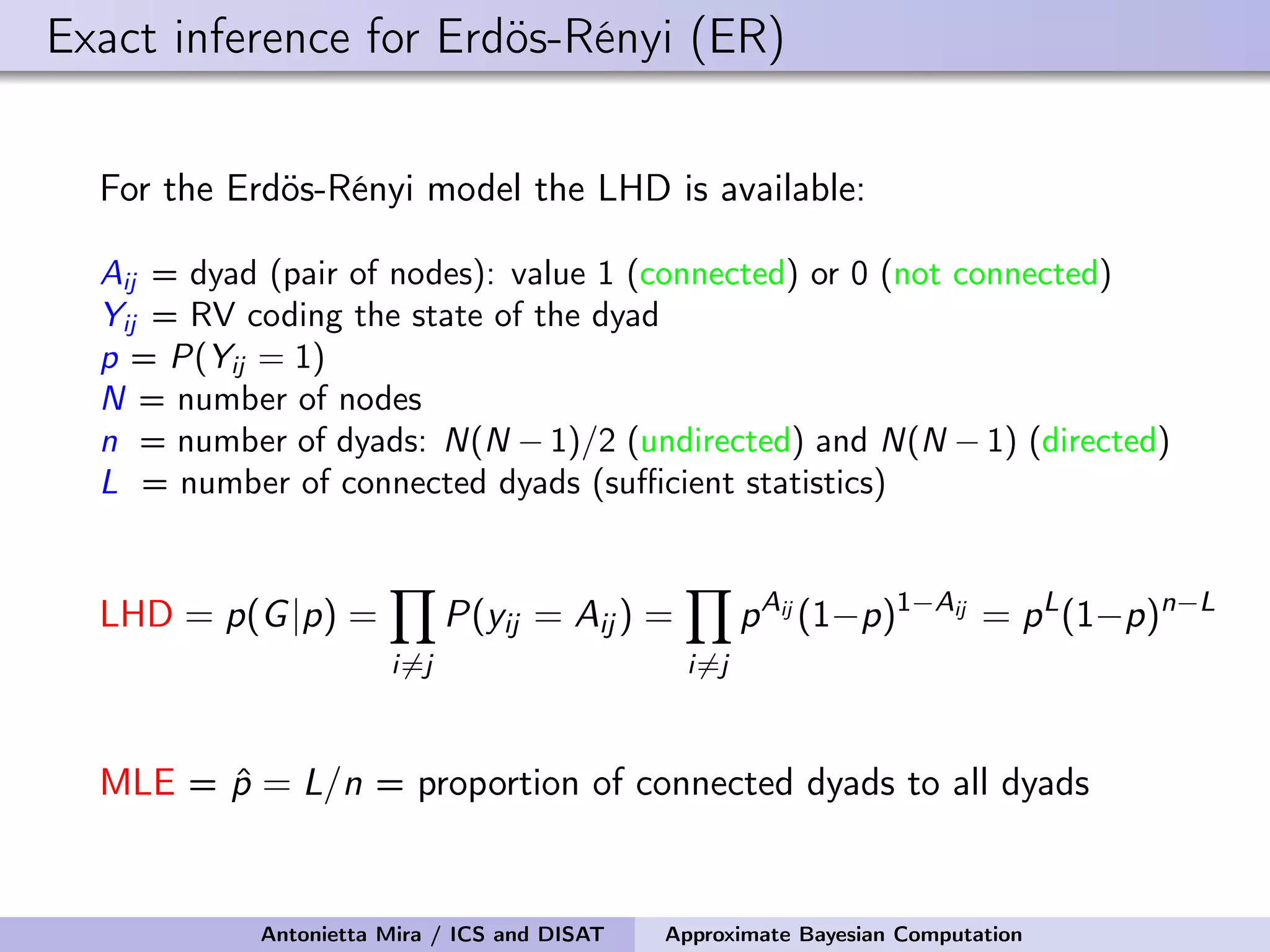
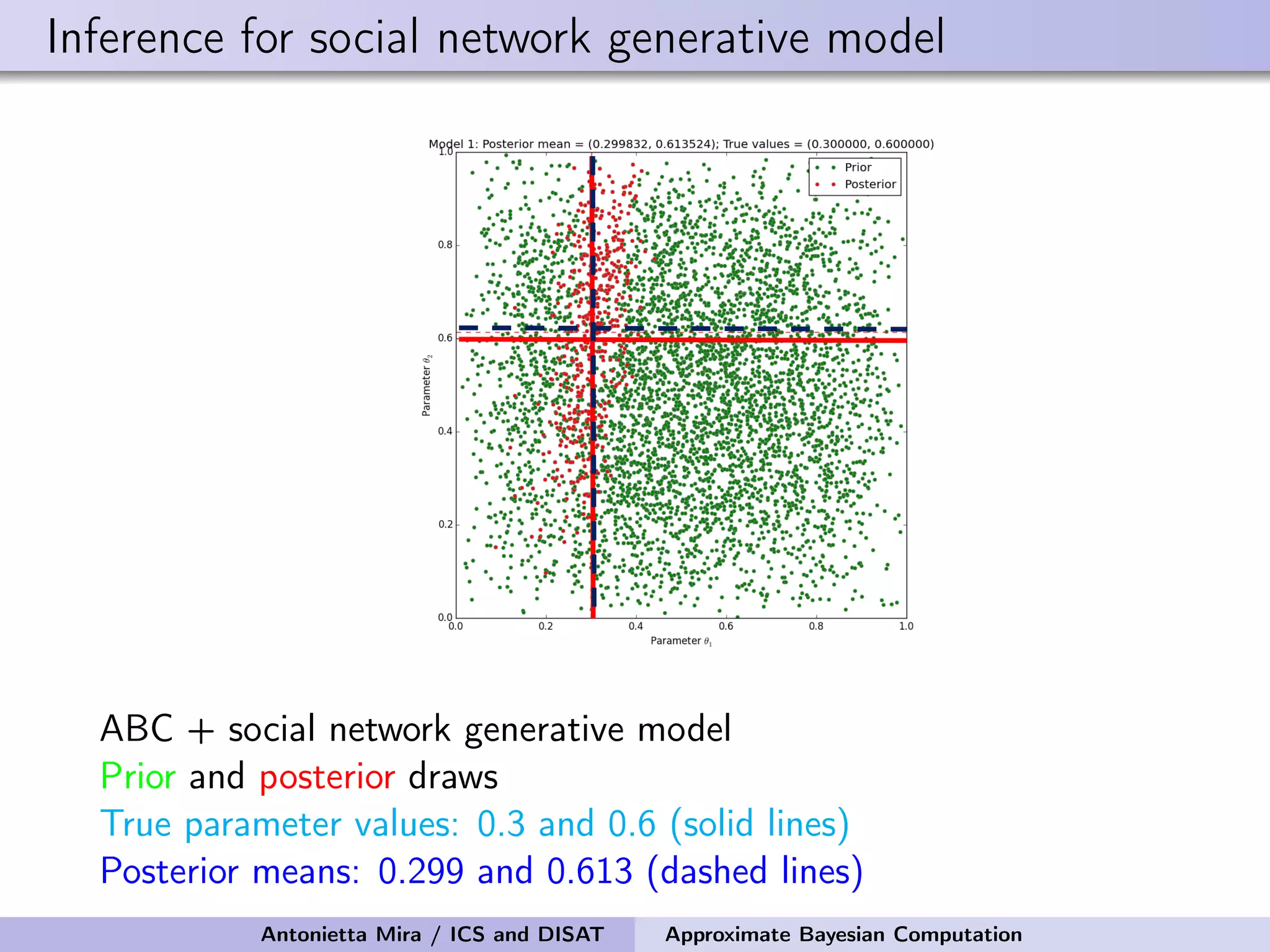
![Approximate Bayesian inference for Erdös-Rényi Pool the distances yk i for all values of i and s: 100, 000 · K total Choose a cutoff value d∗ = 10th percentile Higher acceptance rate: 761 The mean and median of the prior are 0.09 and 0.09 the 95% prior CI is [0.03, 0.18] The mean and median of the posterior are 0.05, 0.05 the 95% posterior CI is [0.04, 0.06] Antonietta Mira / ICS and DISAT Approximate Bayesian Computation](https://image.slidesharecdn.com/mirasamsidec132017-171214220909/75/QMC-Program-Trends-and-Advances-in-Monte-Carlo-Sampling-Algorithms-Workshop-Approximate-Bayesian-Computation-for-Inference-in-Generative-Models-for-Large-scale-Network-Data-Antonietta-Mira-Dec-13-2017-36-2048.jpg)
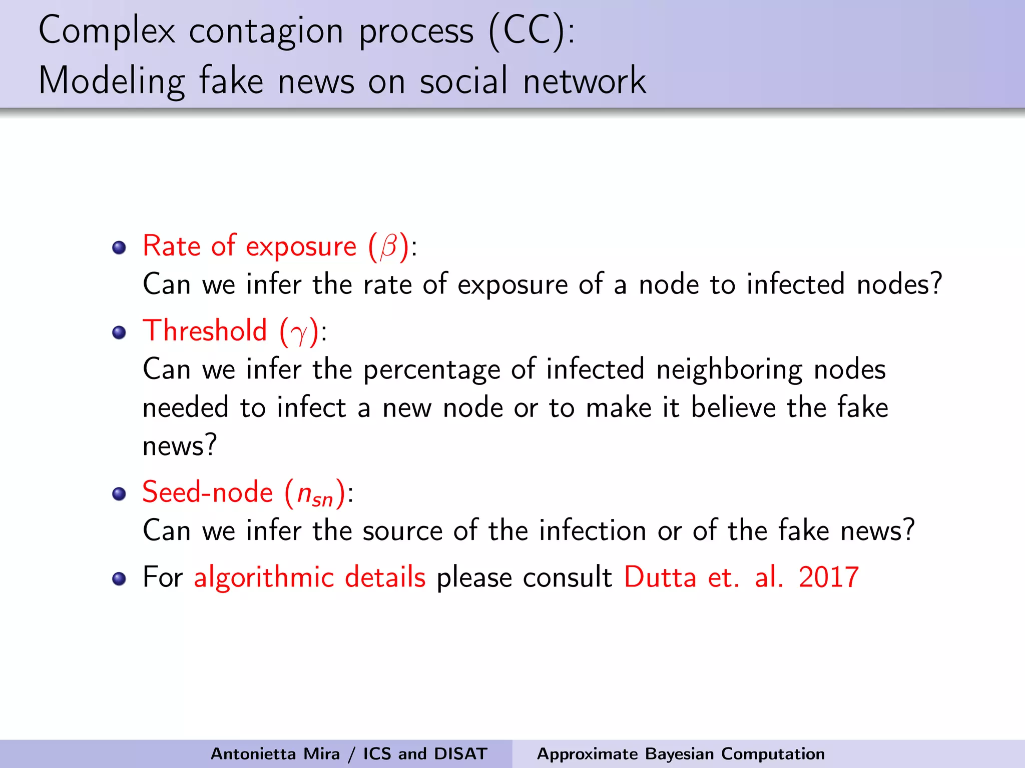
![Details of ABC Prior on the seed node: Uniform on the infected nodes at t1 Prior on the infectivity parameter: Uniform on [0, 1] Perturbation Kernel: A perturbation kernel used to explore the parameter space is defined as a distribution on (θ, nSN) given the present parameter values (θ∗, n∗ SN), K((θ, nSN)|(θ∗, n∗ SN)) = K1(θ|θ∗, ˆσ)K2(nSN|n∗ SN) where K1 = Gaussian with ˆσ being the variance of the θ sampled in the previous step of SABC optimally rescaled K2 = discrete distribution on the neighboring nodes of n∗ SN with each node having a probability inversely proportional to its degree Antonietta Mira / ICS and DISAT Approximate Bayesian Computation](https://image.slidesharecdn.com/mirasamsidec132017-171214220909/75/QMC-Program-Trends-and-Advances-in-Monte-Carlo-Sampling-Algorithms-Workshop-Approximate-Bayesian-Computation-for-Inference-in-Generative-Models-for-Large-scale-Network-Data-Antonietta-Mira-Dec-13-2017-48-2048.jpg)

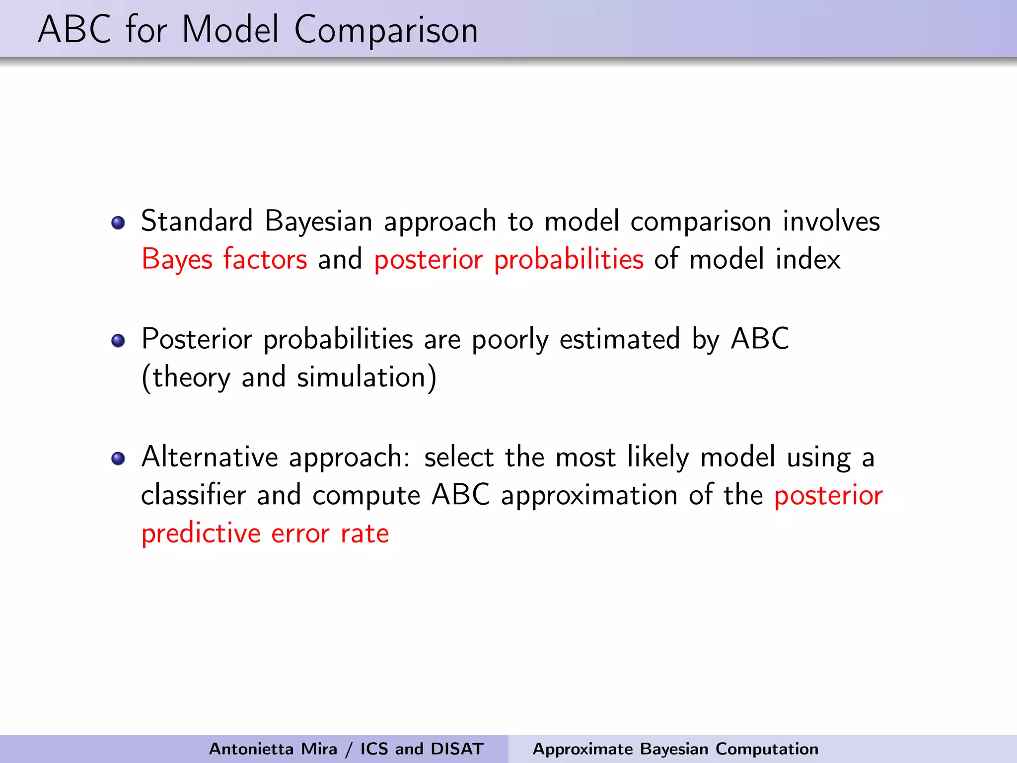
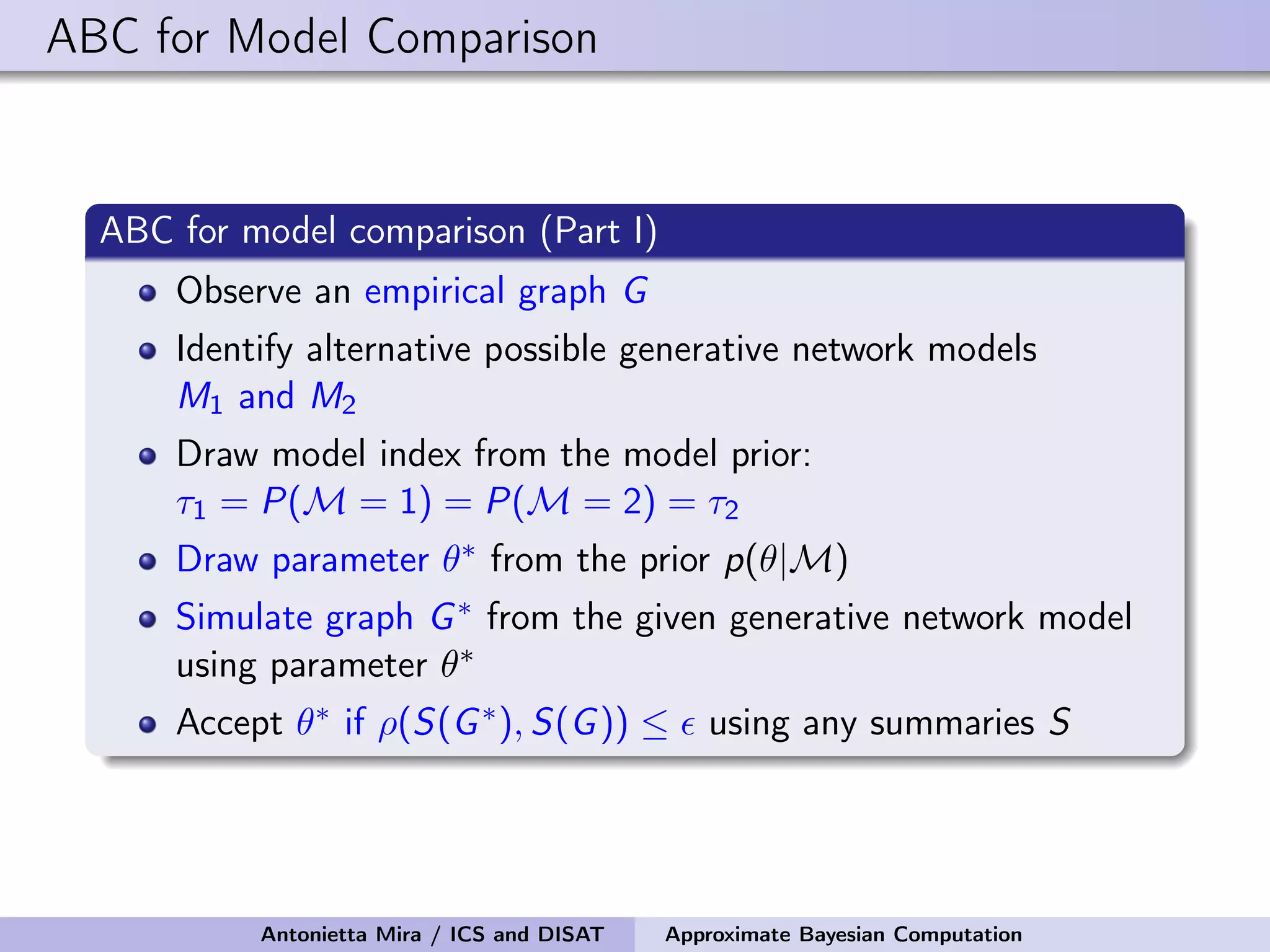
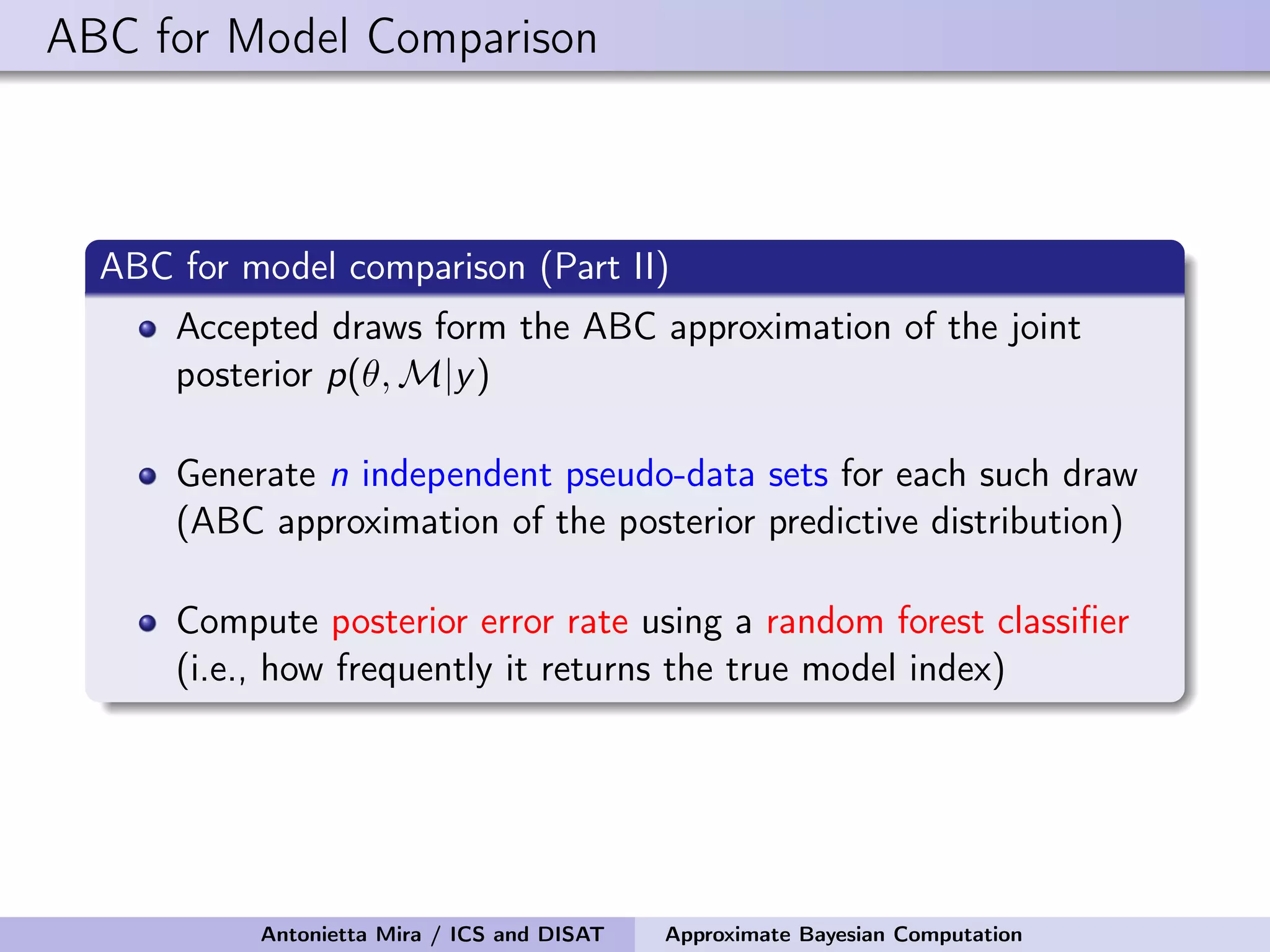
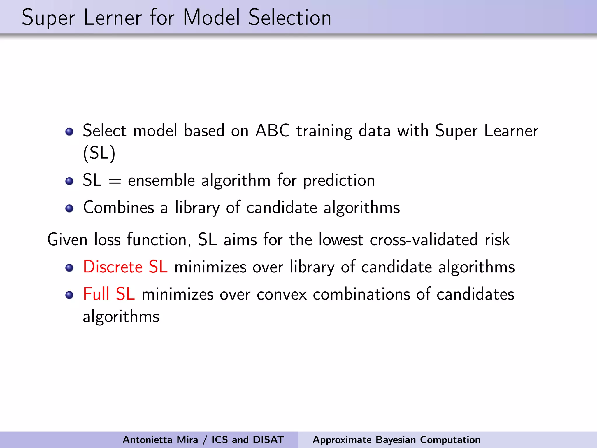
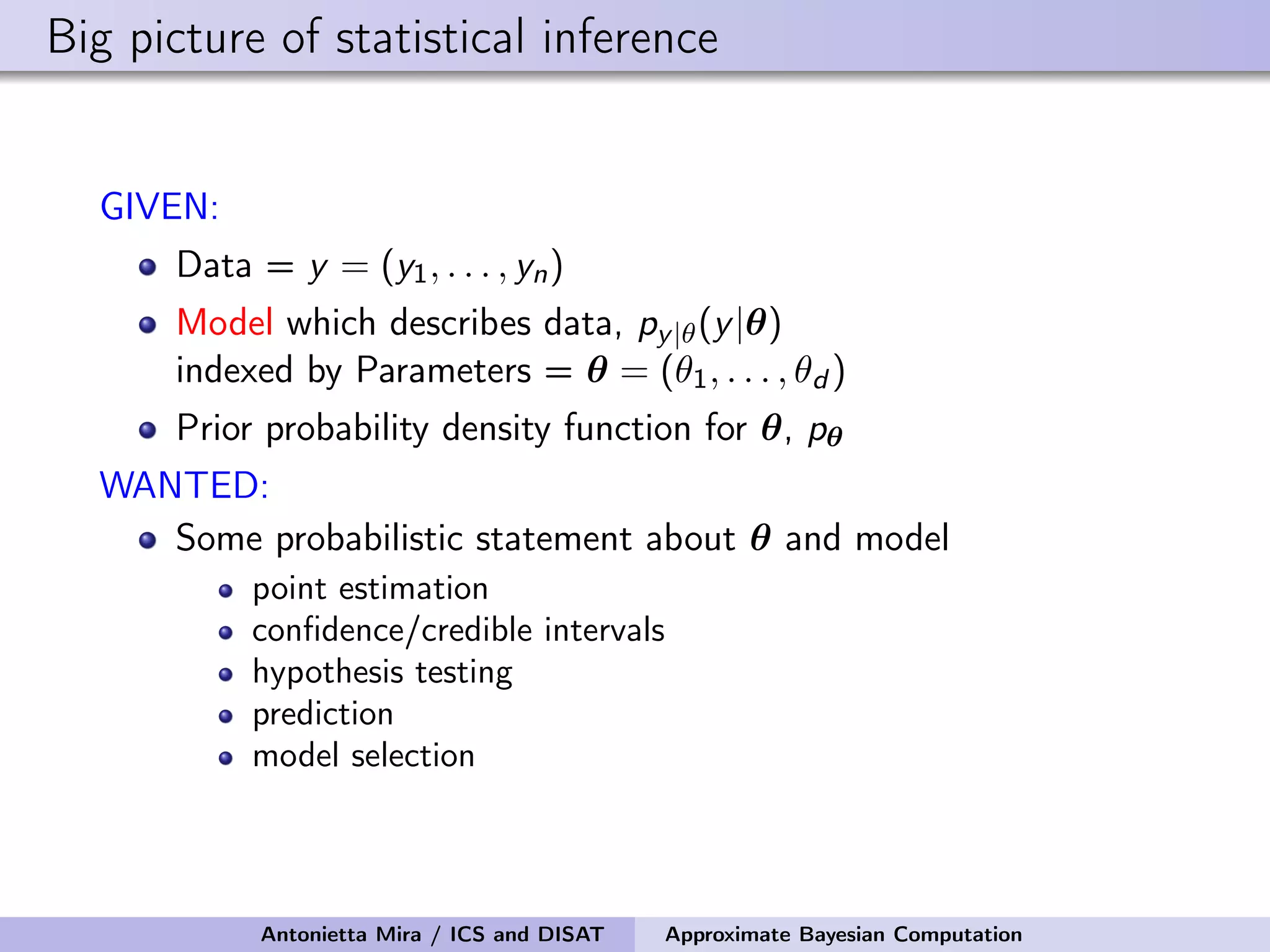
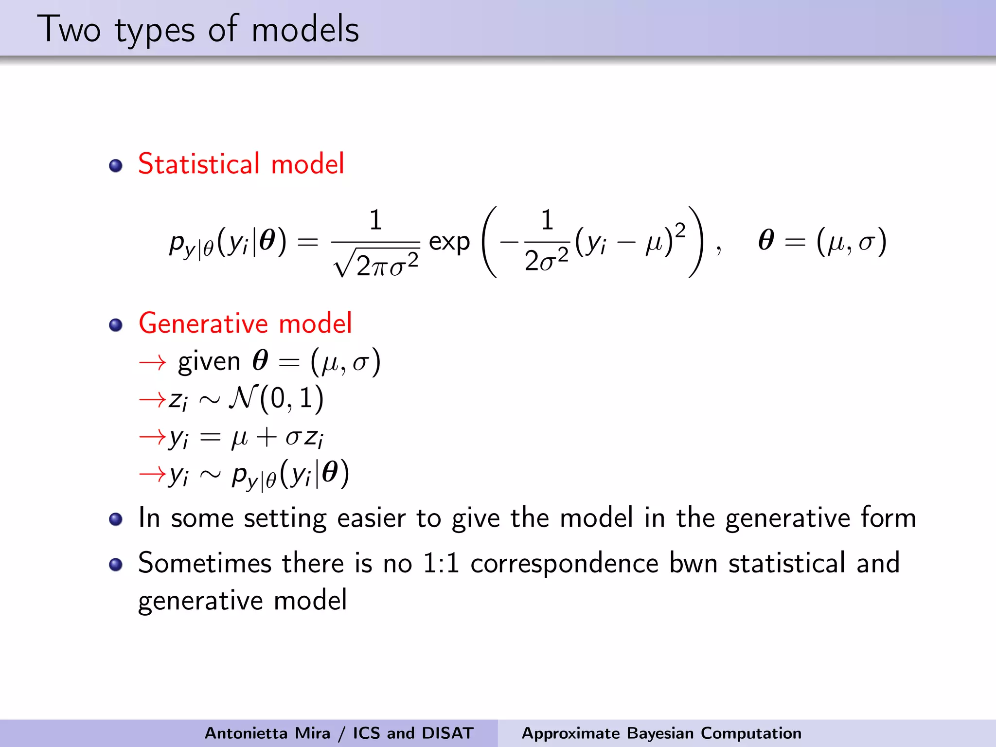
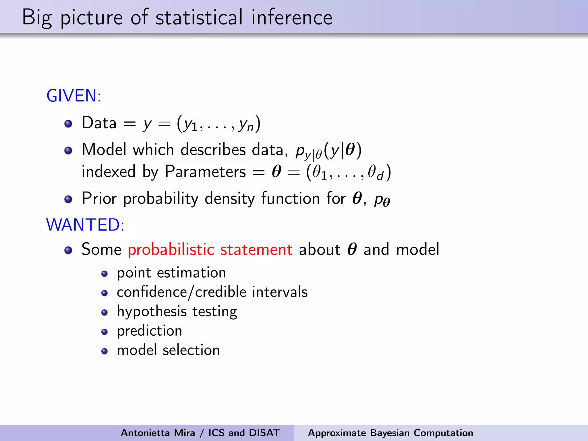
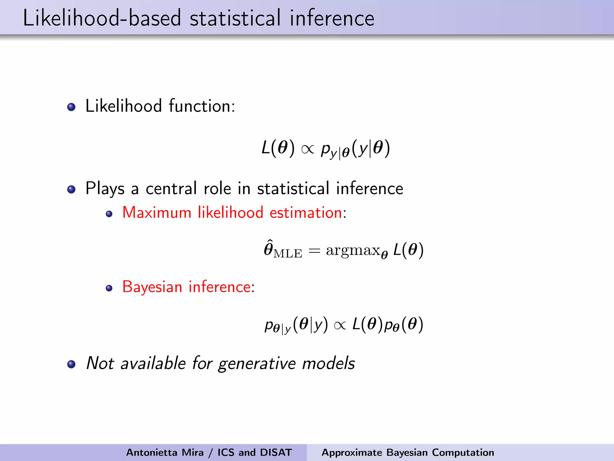
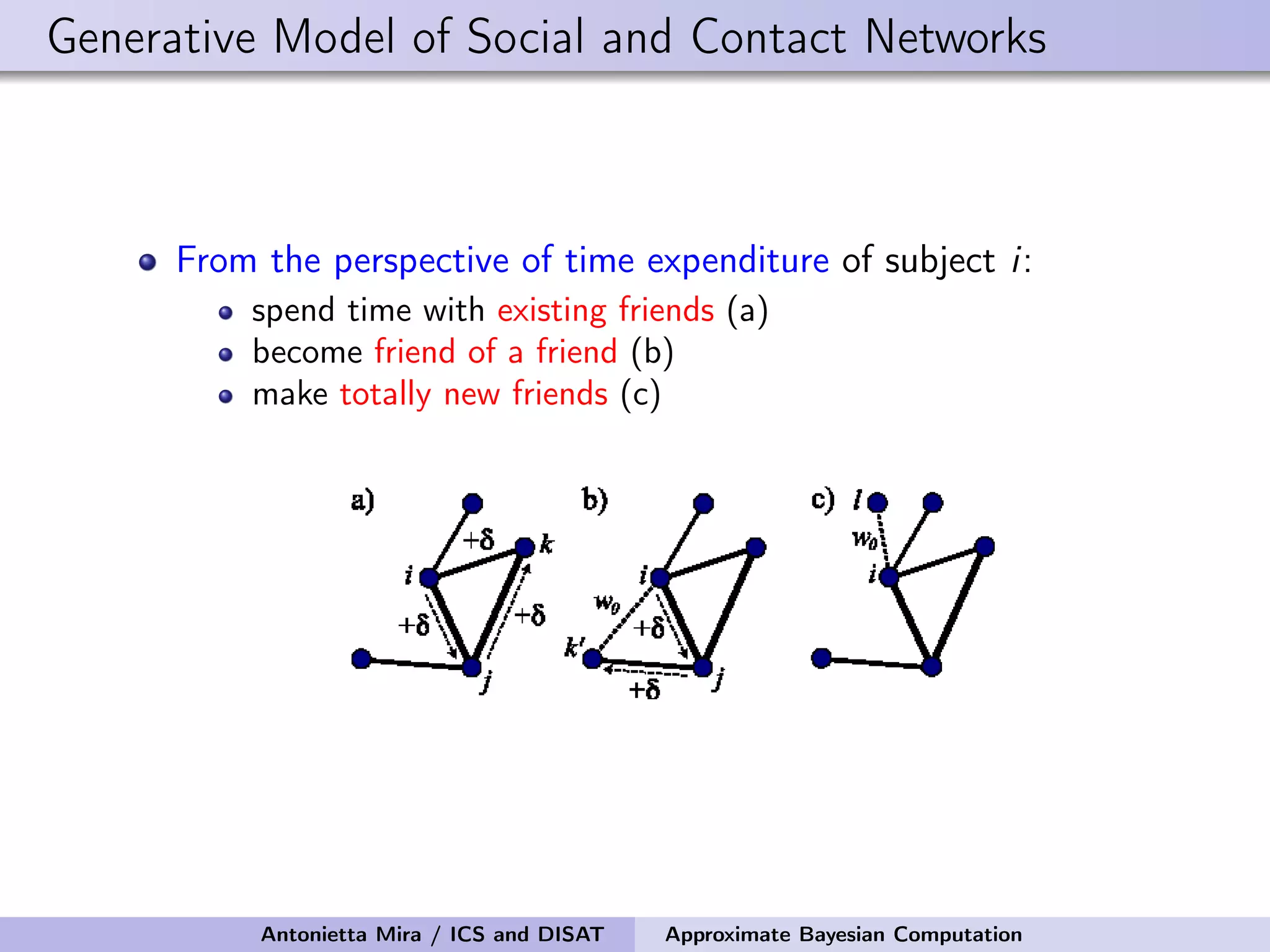
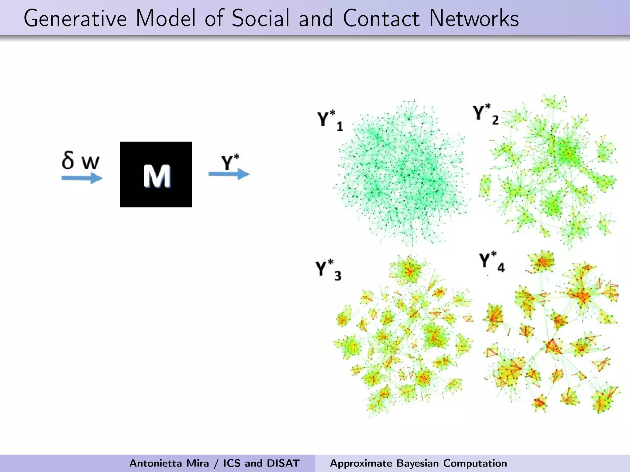
The document discusses the application of Approximate Bayesian Computation (ABC) for inference in generative models, particularly regarding large-scale network data. It highlights the advantages of generative models in terms of scalability and the ability to incorporate domain knowledge, while also addressing challenges in likelihood estimation for network structures. The document provides examples of ABC methodologies and their relevance to various fields, emphasizing the importance of summary statistics in the absence of direct likelihood computation.